Adaptive biases-incorporated latent factorization of tensors for predicting missing data in water quality monitoring networks

Real-time monitoring of key water quality parameters is essential for the scientific management and effective maintenance of aquatic ecosystems. Water quality monitoring networks equipped with multiple low-cost electrochemical and optical sensors generate abundant spatiotemporal data for water authorities. However, large-scale missing data in wireless sensor networks is inevitable due to various factors, which may introduce uncertainties in downstream mathematical modeling and statistical decisions, potentially leading to misjudgments in water quality risk assessment. A high-dimensional and incomplete (HDI) tensor can specifically quantify multi-sensor data, and latent factorization of tensors (LFT) models effectively extract multivariate dependencies and spatiotemporal correlations hidden in such a tensor to achieve high-accuracy missing data imputation. Nevertheless, LFT models fail to adequately account for the inherent fluctuations in water quality data, limiting their representation learning ability. Empirical evidence suggests that incorporating bias schemes into learning models can effectively mitigate underfitting. Building on this insight, this study proposes an adaptive biases-incorporated LFT (ABL) model with four-fold ideas: basic linear biases to describe constant fluctuations in water quality data; weighted pretraining biases to capture historical prior information of data fluctuations; time-aware biases to model long-term patterns of water quality fluctuations; and hyperparameter adaptation via particle swarm optimization (PSO) to enhance practicality. Empirical studies on large-scale real-world water quality datasets demonstrate that the proposed ABL model achieves significant improvements in both prediction accuracy and computational efficiency compared with state-of-the-art models. The findings highlight that integrating multiple bias schemes into tensor factorization models can effectively address the limitations of existing LFT models in capturing inherent data fluctuations, thereby enhancing the reliability of missing data imputation for water quality monitoring. This advancement contributes to more robust downstream applications in water quality management and risk assessment.

1 Introduction

Due to massive industrial production and individual activities, phytoplankton have proliferated rapidly, disrupting the balance of marine and freshwater ecosystems, which is recognized as a matter of global concern [1, 2]. Researchers deploy multi-sensor monitoring networks to assess real-time variation trends of water quality parameters. Indeed, sensor-based monitoring data is precious for water quality prediction and assessment, since continuous observed values with high spatiotemporal resolution is essential to detect slight changes in the ecosystem [3, 4]. However, the issue of missing data is still ubiquitous in real-time monitoring networks, owing to sensor failure, equipment routine maintenance, data corruption, breakdown of data communication, data refinement, and otherwise reasons [5, 6]. The large-scale missing data severely affect the subsequent tasks of statistical analyses and modelling efforts, and even result in misleading decisions to water authorities. Therefore, how to find efficient ways for handling missing data in water quality monitoring networks is urgently needed.

Data reconstruction is an essential strategy to substitute missing values in water quality data. Most current studies attempt to develop prediction approaches for imputing missing water quality data [7]. These techniques range from single imputations that replace each missing value with a precise value to multiple imputations that require consideration of the conditional distribution of missing values within observed data. Recently, machine-learning techniques that can handle multivariate inputs have been adopted to predict large-scale spatiotemporal data [8, 9]. Nevertheless, few works are involved in predicting relevant water quality parameters, especially for real-time monitoring data. It is well known that in-situ online water quality monitoring values are often considered less quantitative than manual measurements due to the inherent fluctuation and nonstationarity of high-frequency readings. For this reason, large-scale missing data from sensor-based networks is a great challenge to solve with conventional machine-learning methods, such as random forest [10], k-nearest neighbors [11], and support vector regression [12]. Moreover, although sophisticated deep-learning techniques can effectively capture multidimensional information and possess strong representation learning abilities, their high computational and storage costs make them impractical in real-world water quality monitoring scenarios, like multi-directional recurrent neural network [13], sequence-to-sequence imputation model [14], and transfer learning-based long short term memory [5]. Hence, there is a significant demand for robust and high-efficiency approaches to predict unobserved values from online monitoring data.

The water quality data generated by a multi-sensor monitoring network can be expressed as a high-dimensional and incomplete (HDI) tensor. Such a tensor can adequately preserve multivariate, spatiotemporal and structural patterns of the original data, giving it inherent advantages in describing water quality parameters [15, 16]. Moreover, a tensor factorization method is gaining attention due to its ability to extract various desired patterns hidden in an HDI tensor [17–20]. To date, a tensor factorization method is successfully applied in diversified areas like quality of service, link prediction, and intelligent transportation system [21–23]. Representative models of this kind include a Candecomp/Parafac (CP) weighted optimization model [17], a fused CP factorization model [18], a regularized tensor decomposition model [19], a non-negative tensor factorization model [20], and a coupled graph-tensor factorization model [56]. Few studies have explored their environmental monitoring applications. To do so, exploring their performance in handling large-scale missing water quality data becomes meaningful.

In general, existing tensor factorization models are efficient in predicting large-scale missing data. However, water quality data display strong fluctuations due to variable transformations and spatiotemporal changes, thereby vastly limiting the representation learning ability of these models. As unveiled by prior studies [24–26], bias schemes can precisely capture inherent fluctuations of complex data to prevent a learning model from underfitting. These methods can handle systematic measurement errors or baseline shifts, enabling a learning model adaptive adjustments to localized anomalies [53, 54]. Specifically, Luo et al. [24] incorporate a basic linear bias scheme into a latent factorization of tensors (LFT) model for perceiving constant data fluctuations. Wu et al. [22] introduce pretraining biases for pre-calculating the statistical deviations between sampled averages and observed values. Xu et al. [54] extend the linear biases on each dimension of tensor for describing more complex data fluctuations. However, existing studies typically employ a single bias scheme to capture data fluctuations caused by a singular factor, fundamentally limiting their representation learning ability in addressing complex water quality data with coupled fluctuation mechanisms. To this end, Yuan et al. [25] prove that the linear combination of different bias schemes can further improve the prediction accuracy of a learning model. Koren et al. [26] integrate time-changing bias scheme and gradual drift bias scheme into a learning model to capture the time-varying fluctuations. Therefore, it is essential to systematically integrate bias schemes into the learning objective.

Inspired by the above studies, this work aims to incorporate reasonable bias schemes into a tensor factorization-based model for achieving accurate prediction of missing water quality data. On the other hand, the hyper-parameters of current tensor factorization-based models are mostly tuned manually through grid-search strategy that consumes immense computing resources and human efforts. Therefore, practical hyper-parameter adaptation mechanism is also desired [27]. To address the above issues, this study innovatively proposes an adaptive biases-incorporated latent-factorization-of-tensors (ABL) model. It seamlessly combines diversified bias schemes with the tensor factorization method to perceive inherent fluctuations of water quality parameters, thereby achieving a robust model with high prediction accuracy for large-scale missing data. Moreover, it designs a reasonable hyper-parameter self-adaptation mechanism to alleviate the resource waste caused by grid-search. By doing so, this work makes the following contributions:

• An ABL model. It combines the merits of diversified bias approaches to integrate three bias schemes into a latent factorization of tensors (LFT) model for ensuring accurate prediction. Furthermore, its hyper-parameters are self-adaptive following the principle of particle swarm optimization (PSO) to enhance practicability.

• Algorithm design and analysis. It offers a specific explanation for researchers to accomplish an ABL model for analyzing large-scale HDI data.

• Detailed empirical studies. We execute experiments on real-world water quality datasets to illustrate that an ABL model exceeds other state-of-the-art models in terms of efficiency and accuracy for predicting missing values.

The rest of this paper consists of the following parts. Section 2 gives the preliminaries. Section 3 provides a detailed description of ABL. Section 4 reports the experimental results. Finally, Section 5 concludes this paper.

2 Preliminaries

2.1 Symbol appointment

Adopted symbols in this study are concluded in Table 1. A variable-station-time tensor is taken as an elementary input data resource when performing missing water quality data prediction. Note that as mentioned in Section 1, the target water quality tensor Y possesses HDI nature, and contains numerous unknown entries due to unobserved monitoring values, the schematic diagram of an HDI water quality tensor is displayed in Figure 1. Thus, we define the target water quality tensor as:

Table 1

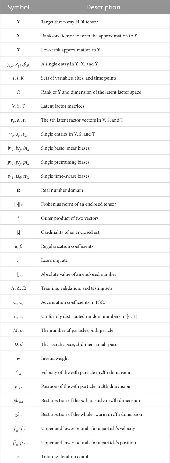
Table 1. Adopted symbols and their descriptions.

Figure 1

Figure 1. An HDI tensor Y of variable-site-time showing water quality parameter values.

Definition 1. (HDI variable-station-time water quality tensor): Given entity sets I, J, and K, let Y^{|I|×|J|×|K|}∈ℝ be a variable-station-time tensor where each entry y_ijk represents a water quality parameter value by variable i∈I on station j∈J at time point k∈K [22, 24]. Y is an HDI tensor if it contains amounts of unknown entries.

2.2 Latent factorization of tensors

In this paper, we achieve LFT on Y in the form of CP tensor factorization, which is actually a special case of Tucker tensor factorization [28, 29]. Compared with CP, although Tucker takes into account entries of a core tensor to realize higher representation ability of a target tensor than CP does, it has the following disadvantages: Tucker consumes more computing resources by noting the extra computational cost proportional to the size of a core tensor, the mathematical form of Tucker is much more complicated to understand than CP [28, 29]. Hence, this work adopts CP tensor factorization as a basic scheme for deriving an LFT model.

With CP tensor factorization, Y is decomposed into R rank-one tensors, that is, X₁, X₂, … , and X_R, where R is the rank of the achieved approximation Ŷ to Y. Identifying R on a given tensor is a nondeterministic polynomial problem [24], it is generally predefined. Specifically, a rank-one tensor is defined as:

Definition 2. (Rank-one Tensor): X_r^{|I| × |J| × |K|} ∈ℝ is a three-way rank-one tensor if it can be written as the outer product of three latent factor (LF) vectors v_r, s_r, t_r with length |I|, |J|, and |K|, respectively [28, 30], as X_r = v_r°s_r°t_r.

Thus, we get the detailed expression of each entry $x_{ijk}^{\left(r\right)}$ in X_r as $x_{ijk}^{\left(r\right)}$ = v_irs_jrt_kr. Subsequently, LF matrices V^|I|×R, S^|J|×R, and T^|K|×R consist of R LF vectors, where the rth column vector in V, S, and T is coupled to form the rth rank-one tensor X_r, as shown in Figure 2. With these R rank-one tensors, we accomplish Y’s rank-R approximation Ŷ as Equation 1:

$\widehat{\mathbf{Y}}={\displaystyle \sum _{r=1}^R}{\mathbf{X}}_r,(1)$

where each entry ŷ_ijk in Ŷ is formulated as:

${\widehat{y}}_{ijk}={\displaystyle \sum _{r=1}^R}{x}_{ijk}^{\left(r\right)}={\displaystyle \sum _{r=1}^R}{v}_{ir}{s}_{jr}{t}_{kr}.(2)$

To gain the expected LF matrices V, S, and T, we construct an objective function ε to measure the difference between Ŷ and Y, which relies on the frequently-used Euclidean distance [21, 26]. It is worth noting that LFT is also compatible with other objective functions [24], such as L_p,q-norms or KL-divergences. With it, the objective function ε is defined as:

$\epsilon ={‖\mathbf{Y}-\widehat{\mathbf{Y}}‖}_F^2={\displaystyle \sum _{i=1}^{\left|I\right|}}{\displaystyle \sum _{j=1}^{\left|J\right|}}{\displaystyle \sum _{k=1}^{\left|K\right|}}{\left(y_{ijk}-{\displaystyle \sum _{r=1}^R}{v}_{ir}{s}_{jr}{t}_{kr}\right)}^2.(3)$

As drawn in Figure 1, Y contains numerous unknown entries. Thus, we define ε on known entry set Λ to denote Y’s known information exactly [30, 31]. Following this, Equation 3 is reformulated into:

$\epsilon ={\displaystyle \sum _{y_{ijk}\in \mathrm{\Lambda }}}{\left(y_{ijk}-{\displaystyle \sum _{r=1}^R}{v}_{ir}{s}_{jr}{t}_{kr}\right)}^2.(4)$

Previous studies have shown that ε is ill-posed due to the imbalanced distribution of Y’s known entries [24, 31]. Thus, we integrate Tikhonov regularization into Equation 4 to enhance its generality:

$\epsilon ={\displaystyle \sum _{y_{ijk}\in \mathrm{\Lambda }}}\left({\left(y_{ijk}-{\widehat{y}}_{ijk}\right)}^2+\alpha {\displaystyle \sum _{r=1}^R}\left(v_{ir}^2+s_{jr}^2+t_{kr}^2\right)\right),(5)$

where α denotes the regularization coefficient for each LF in V, S, and T. Note that ε adopts the density-oriented strategy to build the regularization terms, enabling the model to achieve further generality [32]. By employing a reasonable learning algorithm to minimize the loss in ε [33], an LFT model is achieved. Figure 3 illustrates the process of predicting missing data adopting an LFT model.

Figure 2

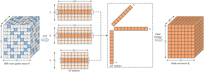
Figure 2. Latent factorization of an HDI tensor Y for handling numerous missing water quality data.

Figure 3

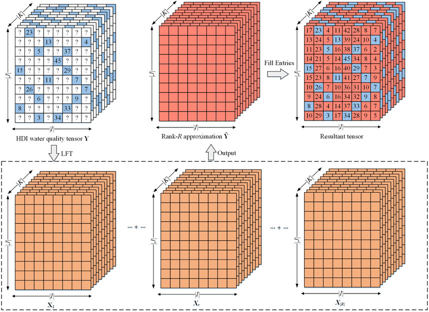
Figure 3. Missing data prediction by performing LFT on a water quality tensor.

2.3 Particle swarm optimization

A PSO algorithm establishes a swarm of M independent particles searching in a D-dimensional space [27, 34]. Each particle is controlled by its velocity vector f_m = [f_m1, f_m2, … , p_mD] and position vector p_m = [p_m1, p_m2, … , p_mD] to find the optimal solution. Following the principle of PSO, the update process of the mth particle at the nth iteration is as follows:

$\begin{array}{l}\forall m\in \left\{1,...,M\right\},d\in \left\{1,...,D\right\}:\\ \left\{\begin{array}{l}{f}_{md}^{\left(n\right)}=w{f}_{md}^{\left(n-1\right)}+{\mathrm{c}}_1{\mathrm{r}}_1\left(p{b}_{md}^{\left(n-1\right)}-p_{md}^{\left(n-1\right)}\right)+{\mathrm{c}}_2{\mathrm{r}}_2\left(g{b}_d^{\left(n-1\right)}-p_{md}^{\left(n-1\right)}\right),\\ p_{md}^{\left(n\right)}=p_{md}^{\left(n-1\right)}+f_{md}^{\left(n\right)}.\end{array}\right.\end{array}(6)$

where w denotes inertia weight, c₁ and c₂ are acceleration coefficients, r₁ and r₂ are uniformly distributed random numbers in [0, 1], pb_md denotes best position of the mth particle in dth dimension, gb_d represents best position of the whole swarm in dth dimension, and PSO iteratively updates the velocity f_md and position p_md of each particle until it meets the convergence conditions.

3 Proposed ABL model

3.1 Diversified bias schemes modeling in LFT

Due to a series of external factors such as seasonal characteristics of parameters, variable transformations, and spatiotemporal changes, water quality data exhibit inherent fluctuations, as shown in Figure 4. According to prior studies [24–26], the representation learning ability and stability of a learning model can be improved by integrating bias schemes into its learning objective, when analyzing such fluctuating data. To this end, we introduce three types of bias schemes into an LFT model for capturing water quality fluctuations.

Figure 4

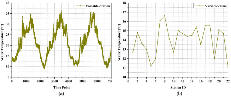
Figure 4. Water quality data fluctuation: (a) values of a particular variable collected by a particular station at different time points, (b) values of a particular variable collected by different sites at the same time point.

In HDI data analysis tasks, the basic linear bias method is commonly employed to prevent a learning model from underfitting [24, 35, 36], which effectively characterizes constant fluctuations of historical data. In our context, for a three-way water quality tensor Y^{|I|×|J|×|K|}, the basic linear biases can be modeled through three bias vectors bv, bs, and bt with length |I|, |J|, and |K|, respectively. By incorporating the corresponding elements in these vectors into Equation 2, we obtain the new entry ŷ_ijk in Ŷ as Equation 7:

${\widehat{y}}_{ijk}={\displaystyle \sum _{r=1}^R}{v}_{ir}{s}_{jr}{t}_{kr}+b{v}_i+b{s}_j+b{t}_k.(7)$

Therefore, the learning objective Equation 5 is reformulated as Equation 8:

$\begin{array}{l}\epsilon ={\displaystyle \sum _{y_{ijk}\in \mathrm{\Lambda }}}\left({\left(y_{ijk}-\left({\displaystyle \sum _{r=1}^R}{v}_{ir}{s}_{jr}{t}_{kr}+b{v}_i+b{s}_j+b{t}_k\right)\right)}^2\right.\\ \left.+\hspace{0.17em}\alpha {\displaystyle \sum _{r=1}^R}\left(v_{ir}^2+s_{jr}^2+t_{kr}^2\right)+\beta \left(b{v}_i^2+b{s}_j^2+b{t}_k^2\right)\right).\end{array}(8)$

Note that the regularization on biases in ε is also connected to each known entry y_ijk∈Λ to reflect the density-oriented strategy.

As indicated in previous research [25, 37, 38], the pretraining bias approach perceives non-stationary fluctuations of known data based on historical prior information before the training process, thereby diminishing the initial error between unobserved values and their corresponding estimates. We reasonably infer that such a method is also applicable for integration into an LFT model. Notice that pretraining biases are not trained together with LFs, but rely on a prior estimator, which may cause their effects on a learning model to be negative in certain iterations. To eliminate the negative effects, we introduce weighted pretraining biases into an LFT model. Thus, each entry ŷ_ijk in Equation 2 is reformulated into Equation 9:

${\widehat{y}}_{ijk}={\displaystyle \sum _{r=1}^R}{v}_{ir}{s}_{jr}{t}_{kr}+{\lambda }_{i}p{v}_i+{\phi }_{j}p{s}_j+{\gamma }_{k}p{t}_k.(9)$

It is worth noting that weight coefficients λ_i, φ_j, and γ_k are trained together with LFs. Since pretraining biases can be acquired by various statistical estimators, and a reasonable estimator is able to enhance the prediction accuracy of a learning model [22, 25]. With it, pv_i, ps_j, and pt_k are formulated as Equation 10:

$\left\{\begin{array}{l}p{v}_i={\displaystyle \sum _{y_{ijk}\in \mathrm{\Lambda }\left(i\right)}}\left(y_{ijk}-\mu \right)/\left({\theta }_1+\left|\mathrm{\Lambda }\left(i\right)\right|\right),\\ p{s}_j={\displaystyle \sum _{y_{ijk}\in \mathrm{\Lambda }\left(j\right)}}\left(y_{ijk}-\mu \right)/\left({\theta }_2+\left|\mathrm{\Lambda }\left(j\right)\right|\right),\\ p{t}_k={\displaystyle \sum _{y_{ijk}\in \mathrm{\Lambda }\left(k\right)}}\left(y_{ijk}-\mu \right)/\left({\theta }_3+\left|\mathrm{\Lambda }\left(k\right)\right|\right),\end{array}\right.(10)$

where Λ(i), Λ(j), and Λ(k) denote subsets of Λ linked with entities i∈I, j∈J, k∈K, respectively. θ₁, θ₂, and θ₃ denote the threshold constants associated with the average of Λ(i), Λ(j), and Λ(k). The global average μ represents the statistical characteristics of Λ [22, 25]. By introducing weighted pretraining biases into Equation 5, yielding Equation 11:

$\begin{array}{l}\epsilon ={\displaystyle \sum _{y_{ijk}\in \mathrm{\Lambda }}}\left({\left(y_{ijk}-\left({\displaystyle \sum _{r=1}^R}{v}_{ir}{s}_{jr}{t}_{kr}+{\lambda }_{i}p{v}_i+{\phi }_{j}p{s}_j+{\gamma }_{k}p{t}_k\right)\right)}^2\right.\\ \left.+\alpha {\displaystyle \sum _{r=1}^R}\left(v_{ir}^2+s_{jr}^2+t_{kr}^2\right)+\beta \left({\lambda }_i^2+{\phi }_j^2+{\gamma }_k^2\right)\right).\end{array}(11)$

Generally speaking, water quality data fluctuate slowly over time. Such a phenomenon indicates that fluctuations of a specific water quality variable between two consecutive collection time points are usually small, while fluctuations between peaks and valleys are commonly obvious, as drawn in Figure 3a. Hence, it is significant to capture the time-changing fluctuation patterns of water quality data to perceive their seasonal and periodic characteristics. Inspired by previous studies [26], this work introduces a time-aware bias approach to describe long-term fluctuations in water quality data. Accordingly, we construct L bins to hold a number of |K| time points, where each bin l∈L puts |K|/L consecutive time points. By doing so, we incorporate these time-aware biases into Equation 2 as Equation 12:

${\widehat{y}}_{ijk}={\displaystyle \sum _{r=1}^R}{v}_{ir}{s}_{jr}{t}_{kr}+t{v}_{il}+t{s}_{jl}+t{t}_{kl}.(12)$

Notice that l∈L corresponds to the bin k∈K belongs to. The objective function ε is obtained as Equation 13:

$\begin{array}{l}\epsilon ={\displaystyle \sum _{y_{ijk}\in \mathrm{\Lambda }}}\left({\left(y_{ijk}-\left({\displaystyle \sum _{r=1}^R}{v}_{ir}{s}_{jr}{t}_{kr}+t{v}_{il}+t{s}_{jl}+t{t}_{kl}\right)\right)}^2\right.\\ \left.+\hspace{0.17em}\alpha {\displaystyle \sum _{r=1}^R}\left(v_{ir}^2+s_{jr}^2+t_{kr}^2\right)+\beta \left(t{v}_{il}^2+t{s}_{jl}^2+t{t}_{kl}^2\right)\right).\end{array}(13)$

Overall, by modeling basic linear biases, weighted pretraining biases, and time-aware biases into an LFT model, we achieve the biases-incorporated learning objective as:

$\begin{array}{l}\epsilon ={\displaystyle \sum _{y_{ijk}\in \mathrm{\Lambda }}}\left({\left(y_{ijk}-{\widehat{y}}_{ijk}\right)}^2+\alpha {\displaystyle \sum _{r=1}^R}\left(v_{ir}^2+s_{jr}^2+t_{kr}^2\right)+\beta \left(b{v}_i^2+b{s}_j^2+b{t}_k^2\right)\right.\\ \left(+\beta \left({\lambda }_i^2+{\phi }_j^2+{\gamma }_k^2\right)+\beta \left(t{v}_{il}^2+t{s}_{jl}^2+t{t}_{kl}^2\right)\right),\end{array}(14)$

where each entry ŷ_ijk is unfolded as Equation 15:

${\widehat{y}}_{ijk}={\displaystyle \sum _{r=1}^R}{v}_{ir}{s}_{jr}{t}_{kr}+\left(b{v}_i+b{s}_j+b{t}_k\right)+\left({\lambda }_{i}p{v}_i+{\phi }_{j}p{s}_j+{\gamma }_{k}p{t}_k\right)+\left(t{v}_{il}+t{s}_{jl}+t{t}_{kl}\right).(15)$

With Equation 14, we derive the objective function of an ABL model. It should be noted that the ABL model only requires approximately (|I| × R+|J| × R+|K| × R) training parameters to represent (|I| × |J| × |K|) samples, significantly saving the computational and storage costs. Next, we present its hyper-parameter adaptation.

3.2 Adaptive parameter learning scheme

When constructing an LFT model, stochastic gradient descent (SGD) is predominantly employed as the learning algorithm to optimize the non-convex objective function of the model by extracting desired LFs and biases, owing to its lightweight structure and efficient implementation [39, 40]. Therefore, we choose SGD as a base algorithm to solve Equation 14. With it, the learning scheme for LFs and biases is derived as:

$\begin{array}{l}\forall i\in I,j\in J,k\in K,l\in L,r\in \left\{1,...,R\right\}\\ \left\{\begin{array}{l}{v}_{ir}\leftarrow v_{ir}\left(1-\eta \alpha \right)+\eta e_{ijk}{s}_{jr}{t}_{kr},b{v}_i\leftarrow b{v}_i\left(1-\eta \beta \right)+\eta e_{ijk},\\ s_{jr}\leftarrow s_{jr}\left(1-\eta \alpha \right)+\eta e_{ijk}{v}_{ir}{t}_{kr},b{s}_j\leftarrow b{s}_j\left(1-\eta \beta \right)+\eta e_{ijk},\\ t_{kr}\leftarrow t_{kr}\left(1-\eta \alpha \right)+\eta e_{ijk}{v}_{ir}{s}_{jr},b{t}_k\leftarrow b{t}_k\left(1-\eta \beta \right)+\eta e_{ijk},\\ {\lambda }_i\leftarrow {\lambda }_i\left(1-\eta \beta \right)+\eta e_{ijk}p{v}_i,t{v}_{il}\leftarrow t{v}_{il}\left(1-\eta \beta \right)+\eta e_{ijk},\\ {\phi }_j\leftarrow {\phi }_j\left(1-\eta \beta \right)+\eta e_{ijk}p{s}_j,t{s}_{jl}\leftarrow t{s}_{jl}\left(1-\eta \beta \right)+\eta e_{ijk},\\ {\gamma }_k\leftarrow {\gamma }_k\left(1-\eta \beta \right)+\eta e_{ijk}p{t}_k,t{t}_{kl}\leftarrow t{t}_{kl}\left(1-\eta \beta \right)+\eta e_{ijk},\end{array}\right.\end{array}(16)$

where e_ijk = y_ijk-ŷ_ijk represents the instant error on y_ijk. Based on Equation 16, we arrive at an SGD-based parameter learning scheme. Notice that a group of controllable hyper-parameters, i.e., η, α, and β, require to be tuned trough grid-search strategy, which is time-consuming and weakens the practicality.

Existing studies indicate that sophisticated optimization algorithms are capable of achieving self-adaptation for a set of hyper-parameters [41–43]. The main advantages of PSO are fast convergence and high compatibility. It is suitable for learning models with multiple hyper-parameters and expensive optimization costs, like an improved LFT model defined on an HDI tensor. Hence, we select PSO to implement hyper-parameters adaptation in Equation 16. To do so, we construct a swarm of M particles in a D-dimensional space, where D = 3 corresponds to η, α, and β. Note that mth particle is applied to the same group of LFs and biases. Equation 17 gives the velocity vector f_m and position vector p_m of mth particle:

$\left\{\begin{array}{l}{\mathit{f}}_m=\left[f_{m1},f_{m2},f_{m3}\right]=\left[f{\eta }_m,f{\alpha }_m,f{\beta }_m\right],\\ {\mathit{p}}_m=\left[p_{m1},p_{m2},p_{m3}\right]=\left[{\eta }_m,{\alpha }_m,{\beta }_m\right].\end{array}\right.(17)$

By substituting it into Equation 6, we realize the evolution strategy of the hyper-parameters. As illustrated in Equation 6, the mth particle evolves based on its personal best position vector pb_m and the global best position vector gb during each iteration, with its update scheme formulated as Equation 18:

$\begin{array}{l}\forall m\in \left\{1,...,M\right\}:\\ \left\{\begin{array}{l}{\mathit{p}\mathit{b}}_m^{\left(n\right)}=\left\{\begin{array}{l}{\mathit{p}\mathit{b}}_m^{\left(n-1\right)},F\left({\mathit{p}\mathit{b}}_m^{\left(n-1\right)}\right)\le F\left({\mathit{p}}_m^{\left(n\right)}\right),\\ {\mathit{p}}_m^{\left(n\right)},F\left({\mathit{p}\mathit{b}}_m^{\left(n-1\right)}\right)>F\left({\mathit{p}}_m^{\left(n\right)}\right);\end{array}\right.\\ {\mathit{g}\mathit{b}}^{\left(n\right)}=\left\{\begin{array}{l}{\mathit{g}\mathit{b}}^{\left(n-1\right)},F\left({\mathit{g}\mathit{b}}^{\left(n-1\right)}\right)\le F\left({\mathit{p}}_m^{\left(n\right)}\right),\\ {\mathit{p}}_m^{\left(n\right)},F\left({\mathit{g}\mathit{b}}^{\left(n-1\right)}\right)>F\left({\mathit{p}}_m^{\left(n\right)}\right).\end{array}\right.\end{array}\right.\end{array}(18)$

To enhance the adaptability of whole swarm to HDI water quality data, we employ the following fitness function as a performance criterion for PSO:

$F=\rho \sqrt{{\displaystyle \sum _{y_{ijk}\in \mathrm{\Psi }}}{\left(y_{ijk}-{\widehat{y}}_{ijk}\right)}^2/\left|\Delta \right|}+\left(1-\rho \right){\displaystyle \sum _{y_{ijk}\in \mathrm{\Psi }}}{\left|y_{ijk}-{\widehat{y}}_{ijk}\right|}_{abs}/\left|\Delta \right|,(19)$

In Equation 19, the balance coefficient ρ is typically set to 0.5 [44], Δ denotes the validation set. Moreover, the velocity and position of each particle need to be constrained within a predefined range, as shown in Equation 20:

$\begin{array}{l}\forall d\in \left\{1,...,D\right\}:\\ \left\{\begin{array}{l}{f}_{md}^{\left(n\right)}=\left\{\begin{array}{l}{\stackrel{͝}{f}}_d,f_{md}^{\left(n\right)}>{\stackrel{͝}{f}}_d,\\ {\stackrel{⌢}{f}}_d,f_{md}^{\left(n\right)}<{\stackrel{⌢}{f}}_d;\end{array}\right.\\ p_{md}^{\left(n\right)}=\left\{\begin{array}{l}{\stackrel{͝}{p}}_d,p_{md}^{\left(n\right)}>{\stackrel{͝}{p}}_d,\\ {\stackrel{⌢}{p}}_d,p_{md}^{\left(n\right)}<{\stackrel{⌢}{p}}_d.\end{array}\right.\end{array}\right.\end{array}(20)$

Furthermore, we set ${\stackrel{͝}{f}}_d=0.2\times \left({\stackrel{͝}{p}}_d-{\stackrel{⌢}{p}}_d\right)$ and ${\stackrel{⌢}{f}}_d=-{\stackrel{͝}{f}}_d$ based on prior research [41].

As a swarm consists of M particles, each evolution iteration is composed of M sub-iterations. Specifically, in the mth sub-iteration of the (n+1) th iteration, the learning rule for LFs and biases is expressed as Equation 21:

$\begin{array}{l}\forall i\in I,j\in J,k\in K,l\in L,r\in \left\{1,...,R\right\},m\in \left\{1,...,M\right\}\\ \left\{\begin{array}{l}{v}_{m,ir}^{\left(n+1\right)}\leftarrow v_{m,ir}^{\left(n\right)}\left(1-{\eta }_m^{\left(n\right)}{\alpha }_m^{\left(n\right)}\right)+{\eta }_m^{\left(n\right)}{e}_{m,ijk}^{\left(n\right)}{s}_{m,jr}^{\left(n\right)}{t}_{m,kr}^{\left(n\right)},b{v}_{m,i}^{\left(n+1\right)}\leftarrow b{v}_{m,i}^{\left(n\right)}\left(1-{\eta }_m^{\left(n\right)}{\beta }_m^{\left(n\right)}\right)+{\eta }_m^{\left(n\right)}{e}_{m,ijk}^{\left(n\right)},\\ s_{m,jr}^{\left(n+1\right)}\leftarrow s_{m,jr}^{\left(n\right)}\left(1-{\eta }_m^{\left(n\right)}{\alpha }_m^{\left(n\right)}\right)+{\eta }_m^{\left(n\right)}{e}_{m,ijk}^{\left(n\right)}{v}_{m,ir}^{\left(n\right)}{t}_{m,kr}^{\left(n\right)},b{s}_{m,j}^{\left(n+1\right)}\leftarrow b{s}_{m,j}^{\left(n\right)}\left(1-{\eta }_m^{\left(n\right)}{\beta }_m^{\left(n\right)}\right)+{\eta }_m^{\left(n\right)}{e}_{m,ijk}^{\left(n\right)},\\ t_{m,kr}^{\left(n+1\right)}\leftarrow t_{m,kr}^{\left(n\right)}\left(1-{\eta }_m^{\left(n\right)}{\alpha }_m^{\left(n\right)}\right)+{\eta }_m^{\left(n\right)}{e}_{m,ijk}^{\left(n\right)}{v}_{m,ir}^{\left(n\right)}{s}_{m,jr}^{\left(n\right)},b{t}_{m,k}^{\left(n+1\right)}\leftarrow b{t}_{m,k}^{\left(n\right)}\left(1-{\eta }_m^{\left(n\right)}{\beta }_m^{\left(n\right)}\right)+{\eta }_m^{\left(n\right)}{e}_{m,ijk}^{\left(n\right)},\\ {\lambda }_{m,i}^{\left(n+1\right)}\leftarrow {\lambda }_{m,i}^{\left(n\right)}\left(1-{\eta }_m^{\left(n\right)}{\beta }_m^{\left(n\right)}\right)+{\eta }_m^{\left(n\right)}{e}_{m,ijk}^{\left(n\right)}p{v}_{m,i}^{\left(n\right)},t{v}_{m,il}^{\left(n+1\right)}\leftarrow t{v}_{m,il}^{\left(n\right)}\left(1-{\eta }_m^{\left(n\right)}{\beta }_m^{\left(n\right)}\right)+{\eta }_m^{\left(n\right)}{e}_{m,ijk}^{\left(n\right)},\\ {\phi }_{m,j}^{\left(n+1\right)}\leftarrow {\phi }_{m,j}^{\left(n\right)}\left(1-{\eta }_m^{\left(n\right)}{\beta }_m^{\left(n\right)}\right)+{\eta }_m^{\left(n\right)}{e}_{m,ijk}^{\left(n\right)}p{s}_{m,j}^{\left(n\right)},t{s}_{m,jl}^{\left(n+1\right)}\leftarrow t{s}_{m,jl}^{\left(n\right)}\left(1-{\eta }_m^{\left(n\right)}{\beta }_m^{\left(n\right)}\right)+{\eta }_m^{\left(n\right)}{e}_{m,ijk}^{\left(n\right)},\\ {\gamma }_{m,k}^{\left(n+1\right)}\leftarrow {\gamma }_{m,k}^{\left(n\right)}\left(1-{\eta }_m^{\left(n\right)}{\beta }_m^{\left(n\right)}\right)+{\eta }_m^{\left(n\right)}{e}_{m,ijk}^{\left(n\right)}p{t}_{m,k}^{\left(n\right)},t{t}_{m,kl}^{\left(n+1\right)}\leftarrow t{t}_{m,kl}^{\left(n\right)}\left(1-{\eta }_m^{\left(n\right)}{\beta }_m^{\left(n\right)}\right)+{\eta }_m^{\left(n\right)}{e}_{m,ijk}^{\left(n\right)},\end{array}\right.\end{array}(21)$

where the subscript m on each parameter denotes that its current state is linked with the mth particle. Consequently, we accomplish an adaptive parameter learning scheme for an ABL model. To clearly demonstrate the training process of ABL, we design a flowchart as shown in Figure 5.

Figure 5

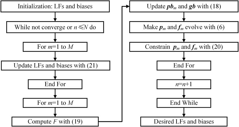
Figure 5. Flowchart of an ABL model.

3.3 Theoretical proof of a bias scheme

This study establishes a rigorous theoretical proof to demonstrate how the bias schemes fundamentally enhance the prediction accuracy of an ABL model. Specially, we employ a basic linear bias scheme as an example. The theoretical proof consists of the following four steps.

Step 1: assuming that an observed value y_ijk in Y can be decomposed into Equation 22:

$y_{ijk}=y_{ijk}^{*}+b{v}_i^{*}+b{s}_j^{*}+b{t}_k^{*},(22)$

where y*_ijk is a low-rank interaction term, bv*_i, bs*_j, and bt*_k are true systematic biases. Thus, we have rank (y* _ijk) = R^*.

Step 2: in a non-biased LFT model, a low-rank approximation value ŷ_ijk requires three factor vectors v_r, s_r, and t_r to fit both systemic biases and interaction term as Equation 23:

${\widehat{y}}_{ijk}={\displaystyle \sum _{r=1}^R}{v}_{ir}{s}_{jr}{t}_{kr}\approx y_{ijk}^{*}+b{v}_i^{*}+b{s}_j^{*}+b{t}_k^{*}.(23)$

Since bv*_i, bs*_j, and bt*_k are essentially rank-one tensors [31], non-biased LFT needs at least R ≥ (R^*+3) to accurately characterize y_ijk, otherwise it inevitably suffer from underfitting. In contrast, a biased LFT model explicitly builds bias terms, and v_r, s_r, and t_r only need to fit y*_ijk as Equation 24:

${\widehat{y}}_{ijk}={\displaystyle \sum _{r=1}^R}{v}_{ir}{s}_{jr}{t}_{kr}+b{v}_i+b{s}_j+b{t}_k\approx y_{ijk}^{*}+b{v}_i^{*}+b{s}_j^{*}+b{t}_k^{*}.(24)$

Hence, a biased LFT model only requires R ≥ R^* to achieve the approximate prediction accuracy as a non-biased LFT model. Consequently, the required rank of LFs in a biased LFT model is reduced, thus intrinsically mitigating underfitting risks.

Step 3: since LFs and biases undergo decoupled optimization, where the bias term governs rapid fitting of systematic biases bv*_i, bs*_j, and bt*_k, while LFs focus on interaction term y*_ijk, thereby ensuring a stable and efficient optimization process.

Step 4: under the premise that step 1 holds, the error upper bound for a biased LFT model is defined as Equation 25:

${‖\mathbf{Y}-\widehat{\mathbf{Y}}‖}_F^2\le {‖{\mathbf{Y}}^{*}-\widehat{\mathbf{Y}}‖}_F^2+{‖{\mathit{b}\mathit{v}}^{*}-\mathit{b}\mathit{v}‖}_2^2+{‖{\mathit{b}\mathit{s}}^{*}-\mathit{b}\mathit{s}‖}_2^2+{‖{\mathit{b}\mathit{t}}^{*}-\mathit{b}\mathit{t}‖}_2^2,(25)$

while the error upper bound for a non-biased LFT model is defined as Equation 26:

${‖\mathbf{Y}-\widehat{\mathbf{Y}}‖}_F^2\le {‖\left({\mathbf{Y}}^{*}+{\mathit{b}\mathit{v}}^{*}+{\mathit{b}\mathit{s}}^{*}+{\mathit{b}\mathit{t}}^{*}\right)-\widehat{\mathbf{Y}}‖}_F^2.(26)$

Therefore, under equivalent rank settings in R^*, a biased LFT model demonstrates strictly lower error upper bound through systematic biases integration.

In summary, this methodological framework fundamentally establishes a biased LFT model’s enhanced imputation accuracy relative to a non-biased LFT model. The derivation methodology extends analogously to the remaining bias schemes.

3.4 Algorithm design and analysis

According to the above inferences, we design the algorithm of an ABL model, as displayed in Algorithm 1, the primary task in each iteration is to update LFs and biases. Consequently, its computational complexity is given as:

$C_{\text{ABL}}\approx \mathrm{\Theta }\left(n\times M\times R\times \left(\left|\mathrm{\Lambda }\right|+\left|\Delta \right|\right)\right).(27)$

Algorithm 1

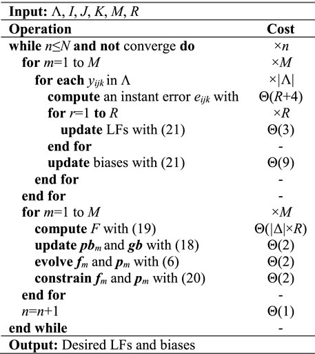
Algorithm 1. ABL.

Equation 27 utilizes the condition that max{|I|, |J|, |K|}≪|Λ|, which is usually satisfied in real applications. Since n, M, and R are positive constants in practice, the computational complexity of an ABL model is linear with (|Λ|+|Δ|) in an HDI tensor. Additionally, according to prior research [30], the computational complexity of an LFT-based model is generally Θ(n × R × (|Λ|+|Δ|)), the only difference is the constant M. The primary reason is that the hyper-parameters in ABL are self-adaptive following the principle of PSO algorithm, whose swarm is made up by M particles. Nevertheless, ABL consumes less iterations to converge. Thus, the proposed model is competitive in computational complexity, which is supported by the experiment results in Section 4.

Its storage complexity relies on three factors: arrays caching the input (|Λ|+|Δ|) and the corresponding estimates, auxiliary arrays caching M independent LFs and biases, and auxiliary arrays caching the storage costs required for hyper-parameter adaptation in PSO. Therefore, by reasonably ignoring lower-order terms and constant coefficients, we achieve the storage complexity of ABL as:

$S_{\text{ABL}}\approx \mathrm{\Theta }\left(\left(\left|I\right|+\left|J\right|+\left|K\right|\right)\times M\times R+\left(\left|\mathrm{\Lambda }\right|+\left|\Delta \right|\right)\right).(28)$

Equation 28 is linear with an HDI tensor’s input count, the swarm size in PSO, and LF count. Section 4 executes experiments to verify the performance of an ABL model.

4 Experimental results and analysis

4.1 General settings

4.1.1 Evaluation metrics

To prevent gradient explosion or disappearance of a learning model caused by inconsistent data magnitude and unit of different water quality parameters, we first adopt a logarithmic normalizer to improve the stability of test models [31]. Then, the evaluation protocol is set as the missing data prediction, which is a widely-used protocol for testing the performance of learning models on HDI tensors. To do so, we adopt root mean squared error (RMSE) and mean absolute error (MAE) as the evaluation metrics [24, 44]:

$\left\{\begin{array}{l}\text{RMSE}=\sqrt{{\displaystyle \sum _{y_{ijk}\in \mathrm{\Omega }}}{\left(y_{ijk}-{\widehat{y}}_{ijk}\right)}^2/\left|\mathrm{\Omega }\right|},\\ \text{MAE}={\displaystyle \sum _{y_{ijk}\in \mathrm{\Omega }}}{\left|y_{ijk}-{\widehat{y}}_{ijk}\right|}_{abs}/\left|\mathrm{\Omega }\right|.\end{array}\right.(29)$

In Equation 29, for a tested model, the smaller RMSE and MAE stand for the higher prediction accuracy.

4.1.2 Experimental data

The online water quality data was collected from 22 monitoring stations in the Three Gorges Reservoir, China. Such a multi-sensor monitoring network obtains eight important water quality parameters, including water temperature (°C), pH, dissolved oxygen (mg/L), electrical conductivity (μS/cm), turbidity (NTU), chemical oxygen demand (mg/L), total phosphorus (mg/L), and total nitrogen (mg/L). Their collected frequency was set to every 4 hours from 1 January 2020 to 30 June 2023, resulting in 7662 consecutive sampling points. Subsequently, we get a water-quality tensor with the size of 22 × 8 × 7662. The dataset contains 1,248,061 samples, and the data density is about 92.55%, which is high compared with most practical applications. Thus, in the experiments, we build four simulated testing cases, their detailed information is shown in Table 2. Notice that the data density in Table 2 is calculated by Equation 30:

$\text{Density}=\frac{\left|\mathrm{\Lambda }\right|+\left|\Delta \right|}{\left|\mathrm{V}\right|\times \left|\mathrm{S}\right|\times \left|\mathrm{T}\right|}\times 100\%.(30)$

Table 2

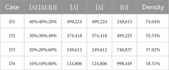
Table 2. Detailed settings of testing cases.

Specifically, considering D1, its |Λ|:|Δ|:|Ω| is 40%:40%:20%, representing that we randomly choose 40% from 1,248,061 samples as training set Λ and 40% as validation set Δ to establish a learning model, the remaining 20% as testing set Ω to verify the performance of each model. For each testing case, the random splitting of |Λ|, |Δ| and |Ω| is repeated for 50 times to obtain 50 independent experimental sets for eliminating possible deviations caused by data splitting. Moreover, the standard deviations metric is included in the analysis [30]. As one of the core metrics for quantifying prediction uncertainty, it specifically characterizes the dispersion of prediction values around their mean. A larger standard deviation indicates lower reliability of the prediction values. This metric directly determines the width of the confidence interval, thereby quantifying the confidence range of the prediction results. For all tested models, the LF space dimension R is fixed at 20 to balance the computational cost and prediction accuracy [31], and PSO-related parameters are consistent with empirical values [34], i.e., M = 10, w = 0.729, and c1 = c2 = 2. Moreover, to avoid gradient disappearance or explosion of learning models caused by inconsistent value ranges of different water quality variables, we employ a normalizer for each entry y_ijk to improve the stability of the experimental results [31].

4.1.3 Training settings

The training process of a tested model terminates if its expended iteration count arrives 1,000, or the training error difference between two consecutive iterations is less than 10⁻⁵. The training error of a model is tested on Δ. Its output RMSE and MAE are tested on Ω. All tested models are executed on a server equipped with a 3.2 GHz i5 CPU and 128 GB RAM, adopting JAVA SE 7U60 as the operating platform.

4.2 Hyper-parameter sensitivity

In this section, we validate the effects of hyper-parameter adaptation in an ABL model. For this purpose, we omit the hyper-parameter adaptation component from an ABL model, and tune these hyper-parameter through manual grid-search to obtain the optimal predictive performance. The searching range and its optimal hyper-parameters for the grid-search strategy are recorded in Table 3. Subsequently, we compare the performance of manual grid-search and PSO-based adaptation, with the comparison results presented in Table 4. The experimental results clearly demonstrate the positive effects by the hyper-parameter adaptation in an ABL model. From it, we get some important findings.

Table 3

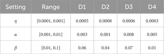
Table 3. Searching range and optimal values via grid-search.

Table 4

Table 4. Performance comparison between two methods in RMSE and MAE.

With hyper-parameter adaptation, an ABL model substantially improves its prediction accuracy. For instance, as shown in Table 4, the MAE of an ABL model with PSO-based adaptation is 0.1739 on D4, while the MAE of an ABL model with manual grid-search is 0.1843. Hence, the hyper-parameter adaptation enables an ABL model to accomplish the accuracy gain at 5.64%. Similar results are encountered on other testing cases. The primary reason is that the grid-search strategy fixes hyper-parameters throughout the training process, potentially causing the model to converge to suboptimal local minima. Conversely, PSO-based adaptation dynamically adjust hyper-parameters at a finer granularity, enabling the model to escape local optima and realize superior solutions.

An ABL model’s hyper-parameter adaptation alleviates the time cost immensely. It can be seen from Table 4 that the time cost of an ABL model with manual grid-search is comparable with that of an ABL model with PSO-based adaptation. Nevertheless, seeking the optimal hyper-parameters through grid-search is time-consuming. For instance, on D1, the grid-search strategy consumes 7683 s to choose the optimal hyper-parameters to arrive the lowest RMSE, which is about 452 times of that by PSO-based adaptation. Other testing cases yield similar results, as recorded in Table 4.

It should be noted that the time cost per iteration for an ABL model with PSO-based adaptation is significantly higher than that of an ABL model with manual grid-search, whereas its convergence iteration count is substantially lower. This is attributed to the PSO algorithm’s structure, where each iteration comprises M sub-iterations to evolve hyper-parameters. Consequently, the time cost per iteration is approximately M times that of grid-search, but the iteration count and overall time cost are dramatically reduced.

4.3 Comparison with state-of-the-art models

This set of experiments compares an ABL model with several state-of-the-art models to verify its performance. Their details are as follows:

M1: A CP-weighted optimization model [17]. It adopts a first-order optimization method to solve the weighted least squares issue.

M2: A non-negative tensor factorization model [20]. It adopts CP to complete an HDI tensor with the consideration of non-negativity, and updates LFs via a multiplicative update scheme.

M3: A high-dimension-oriented prediction model [21]. It models multi-dimensional data via concepts of tensor, and predicts the missing data via reconstructed optimization algorithms.

M4: A tensor completion model [45]. It employs a gradient descent-based mechanism to enhance the prediction accuracy by imputing the missing entries in an HDI tensor.

M5: A depth-adjusted non-negative LFT model [30]. It presents a joint learning-depth-adjusting strategy to escape frequent training fluctuation and weak model convergence.

M6: A biased non-negative LFT model [24]. It integrates linear biases into the model for describing fluctuations, and designs a non-negative multiplicative update rule to update LFs and biases.

M7: An SGD-based LFT model [36]. It utilizes SGD algorithm as its parameter learning scheme, and incorporates bias terms to improve its prediction accuracy.

M8: An ABL model proposed in this paper. It presents diversified biases to capture inherent fluctuations in water quality data, and introduces PSO-based adaptation to boost its practicability.

Figure 6 records each compared model’s convergence iteration count. Table 5 illustrates their time costs. Table 6 depicts the RMSE and MAE of the compared models. From these results, we draw several interesting findings.

Figure 6

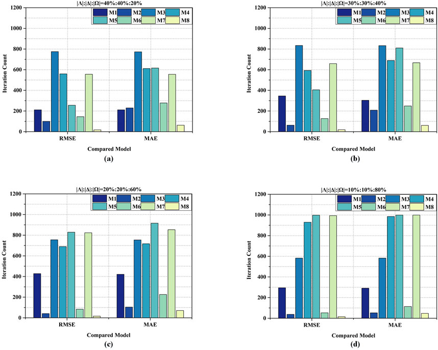
Figure 6. Convergence iteration count of eight models on four testing cases: (a) iteration count on D1, (b) iteration count on D2, (c) iteration count on D3, (d) iteration count on D4.

Table 5

Table 5. Time cost of each compared model in seconds.

Table 6

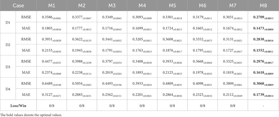
Table 6. Lowest RMSE and MAE of each compared model.

M8, i.e., a proposed ABL model, converges much faster than its peers do. According to Figure 6a, M8 only takes 18 iterations to complete the convergence in RMSE, while M1-M7 takes 212, 100, 775, 559, 256, 145 and 556 iterations to achieve the convergence in RMSE on D1, respectively. As for MAE, as shown in Figure 6b, M1-M7 consume 304, 208, 833, 689, 810, 249 and 667 iterations, respectively, to ensure model convergence on D2. By contrast, M8 requires only 61 iterations. Similar results can be found on D3 and D4, as displayed in Figures 6c,d. From these results, we can clearly see that the convergence rate of an ABL model is significantly higher than its peers. Therefore, utilizing the PSO-based adaption in an LFT-based model is feasible and high-efficiency.

M8 achieves remarkable efficiency gain over the advanced models. As depicted in Table 5, M8 realizes the lowest time cost on four testing cases. For instance, on D4, M8 consumes about 13 s to converge in MAE, which is 3.76% of 346 s by M1, 48.15% of 27 s by M2, 3.88% of 335 s by M3, 3.03% of 429 s by M4, 2.90% of 449 s by M5, 25% of 52 s by M6, and 32.50% of 40 s by M7. Similar outputs are gained on D1-D3. As shown in Algorithm 1, the computational cost of an ABL model chiefly depends on an HDI water quality tensor’s known entries. Moreover, its PSO-based adaptation possesses fast convergence and high compatibility. Hence, we can conclude that such a modeling strategy is highly appropriate for analyzing large-scale water quality data.

M8 exhibits strong competitiveness in predicting large-scale missing water quality data. As recorded in Table 6, M8 acquires the lowest predication error across all testing cases. For instance, on D1, M8 realizes the lowest MAE at 0.1473, which is about 18.30% lower than 0.1803 by M1, 17.11% lower than 0.1777 by M2, 14.16% lower than 0.1716 by M3, 13.50% lower than 0.1699 by M4, 14.56% lower than 0.1724 by M5, 11.53% lower than 0.1665 by M6, and 12.01% lower than 0.1674 by M7. Furthermore, on D4, M8 achieves the lowest RMSE at 0.3068, which is about 52.72% lower than 0.6489 by M1, 39.30% lower than 0.5054 by M2, 31.72% lower than 0.4493 by M3, 21.99% lower than 0.3933 acquired by M4, 36.20% lower than 0.4809 acquired by M5, 25.13% lower than 0.4098 acquired by M6, 19.45% lower than 0.3809 by M7. A similar phenomenon are achieved on D2 and D3. The primary reason for M8’s performance gain lies in its integration of diversified biases to characterize inherent fluctuations in water quality data, combined with a PSO-based hyper-parameter adaptation mechanism that enhances the fitting for an HDI tensor. Thus, M8 possesses highly competitive prediction accuracy for large-scale missing water-quality data.

The performance gain of M8 is statistically significant in our experiments. To further measure the performance of the above compared models, we employ the Friedman test [46] to verify their statistical significance given in Tables 5, 6. The average rankings of efficiency and accuracy across compared models are compiled in Table 7. Assuming that go p is the ranking of the compared model on corresponding testing case, where o represents the oth one of O compared models and p represents the pth one of P testing cases. The Friedman test calculates the average ranking of each model’s performance on all testing cases, i.e., $H_o={\displaystyle {\sum }_{p=1}^P}{g}_p^o/P$. Then, we compute the Friedman value as Equation 31:

${\chi }_F^2=\frac{12P}{O\left(O+1\right)}\left[{\displaystyle \sum _{o=1}^O}{H}_o^2-\frac{O{\left(O+1\right)}^2}{4}\right].(31)$

Table 7

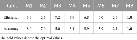
Table 7. Average ranking of all compared models.

Subsequently, the testing score is given as Equation 32:

$F_F=\frac{\left(P-1\right){\chi }_F^2}{P\left(O-1\right)-{\chi }_F^2}.(32)$

Notice that the testing score conforms to the F-distribution with (O-1) and (O-1) (P-1) degrees of freedom [44]. Thus, if F_F is higher than the corresponding critical, we can reject the null hypothesis with the critical level σ.

For instance, to compare accuracy, eight models are tested on eight testing cases, i.e., O=P=8, and the degrees of Friedman freedom for F_F is (7, 49). If we set σ = 0.05, the critical value of F (7, 49) is 2.20. Hence, the null hypothesis is rejected if the testing score F_F is greater than 2.20. According to Tables 5, 6, we calculate that the testing score of efficiency is 61.67, which is obviously higher than the critical value of 2.20. Similarly, when we set σ = 0.05, the critical value of F (7,49) for accuracy is also 2.20 and the testing score is 240.58. Therefore, we prove that M1-M8 have a remarkable performance difference at the 95% confidence level. As recorded in Table 7, we can accurately deduce that M8 has the lowest average ranking values, which denotes that it outperforms its peers in terms of prediction accuracy and computational efficiency.

For further validating M8’s performance gain, we consider the Nemenyi analysis [46], whose main idea is that if the ranking difference between arbitrary two models is more significant than the critical value, the performance of the two models is significantly different. The critical value is formulated as Equation 33:

$CD=q_{\sigma }\sqrt{\frac{O\left(O+1\right)}{6P}},(33)$

where the constant q_σ is based on the studentized range statistics [46]. With eight compared models, we get a critical value q_σ = 2.78 with the critical level σ = 0.1 [25]. Regarding efficiency, by substituting O=P=8, we gain CD = 3.40, which means that two models with a ranking difference greater than 3.40 have significantly different in performance with a confidence level at 90%.

From the Nemenyi analysis results depicted in Figure 7, M8 obviously outperforms M1, M3, M4, and M5 according to computational efficiency. Considering prediction accuracy, M8 significantly outperforms all compared models except M4, M6 and M7. Therefore, we conclude that an ABL model is competitive in prediction accuracy and computational efficiency.

Figure 7

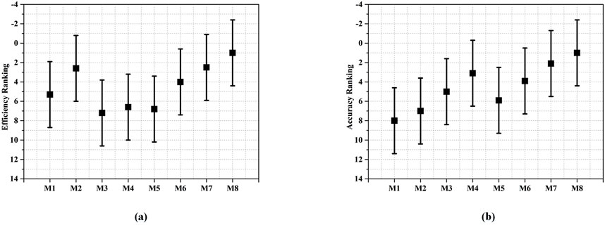
Figure 7. Results of Nemenyi analysis: (a) efficiency of M1-8, (b) accuracy of M1-8.

5 Conclusion

This study aims at precisely representing an HDI water quality data, thereby realizing high efficiency and accuracy for large-scale missing water quality data prediction. To do so, we propose an ABL model. It incorporates diversified biases into an LFT model to precisely describe the inherent fluctuations hidden in water quality data. Moreover, it executes PSO-based adaptation to reduce the time costs caused by hyper-parameter tuning. Compared to state-of-the-art models designed for HDI data, an ABL model achieves higher computational efficiency and prediction accuracy.

Considering the future plans, the following issues need to be addressed. Firstly, more advanced hyper-parameter adaptation algorithms [47, 48] may be compatible with an ABL model to achieve better performance gain. Secondly, due to the diversity of bias schemes [49, 50], how to design a robust ensemble framework to further perceive the inherent fluctuations in water quality data is still a meaningful challenge. Additionally, the computational efficiency of an ABL model may be significantly improved through parallel computing techniques [51, 52], enabling its application to high-volume online water quality monitoring datasets. Moreover, since real-world water quality data generally contain additional attributes like depth profile, which a higher-order tensor can naturally describe [55], extending the proposed model to handle such a tensor can further validate the model’s applicability in complex environments. We plan to address these issues in our future work.

Data availability statement

The raw data supporting the conclusions of this article will be made available by the authors, without undue reservation.

Author contributions

XW: Conceptualization, Data curation, Formal Analysis, Investigation, Methodology, Software, Validation, Visualization, Writing – original draft. LW: Data curation, Formal Analysis, Investigation, Project administration, Validation, Visualization, Writing – review and editing. MG: Data curation, Investigation, Project administration, Software, Writing – review and editing. JJ: Investigation, Project administration, Supervision, Writing – review and editing. YC: Resources, Supervision, Writing – review and editing. BY: Funding acquisition, Supervision, Writing – review and editing.

Funding

The author(s) declare that financial support was received for the research and/or publication of this article. This research was supported by the Chongqing Science and Technology Commission (CSTB2024NSCQ-MSX0625), Special Project for Performance Incentive Guidance of Chongqing Scientific Research Institutions (CSTB2024JXJL-YFX0075, CSTB2023JXJL-YFX0054), Scientific and Technological Research Program of Chongqing Municipal Education Commission (KJQN202401610), Environmental Monitoring Research and Development Fund (COHJ-NBKY-2023-002, COH-NBKY-2023-012).

Conflict of interest

The authors declare that the research was conducted in the absence of any commercial or financial relationships that could be construed as a potential conflict of interest.

Generative AI statement

The author(s) declare that no Generative AI was used in the creation of this manuscript.

Publisher’s note

All claims expressed in this article are solely those of the authors and do not necessarily represent those of their affiliated organizations, or those of the publisher, the editors and the reviewers. Any product that may be evaluated in this article, or claim that may be made by its manufacturer, is not guaranteed or endorsed by the publisher.

References

1. Conley D, Paerl H, Howarth R, Boesch D, Seitzinger S, Havens K, et al. Controlling eutrophication: nitrogen and phosphorus. Science (2009) 323:1014–5. doi:10.1126/science.1167755

PubMed Abstract | CrossRef Full Text | Google Scholar

2. Zhao K, Wang L, You Q, Pan Y, Liu T, Zhou Y, et al. Influence of cyanobacterial blooms and environmental variation on zooplankton and eukaryotic phytoplankton in a large, shallow, eutrophic lake in China. Sci Total Environ (2021) 773:145421. doi:10.1016/j.scitotenv.2021.145421

PubMed Abstract | CrossRef Full Text | Google Scholar

3. Marcé R, George G, Buscarinu P, Deidda M, Dunalska J, de Eyto E, et al. Automatic high frequency monitoring for improved lake and reservoir management. Environ Sci Technology (2016) 50:10780–94. doi:10.1021/acs.est.6b01604

PubMed Abstract | CrossRef Full Text | Google Scholar

4. Shan K, Ouyang T, Wang X, Yang H, Zhou B, Wu Z, et al. Temporal prediction of algal parameters in Three Gorges Reservoir based on highly time-resolved monitoring and long short-term memory network. J Hydrol (2022) 605:127304. doi:10.1016/j.jhydrol.2021.127304

CrossRef Full Text | Google Scholar

5. Chen Z, Xu H, Jiang P, Yu S, Lin G, Bychkov I, et al. A transfer learning-based LSTM strategy for imputing large-scale consecutive missing data and its application in a water quality prediction system. J Hydrol (2021) 602:126573. doi:10.1016/j.jhydrol.2021.126573

CrossRef Full Text | Google Scholar

6. Dagtekin O, Dethlefs N. Imputation of partially observed water quality data using self-attention LSTM. In: Proceedings of the 2022 IEEE international joint conference on neural networks (2022). p. 1–8. doi:10.1109/ijcnn55064.2022.9892446

CrossRef Full Text | Google Scholar

7. Zhang Y, Thorburn P. Handling missing data in near real-time environmental monitoring: a system and a review of selected methods. Future Generation Computer Syst (2022) 128:63–72. doi:10.1016/j.future.2021.09.033

CrossRef Full Text | Google Scholar

8. Baggag A, Abbar S, Sharma A, Zanouda T, Mohan A, Ai-Homaid A, et al. Learning spatiotemporal latent factors of traffic via regularized tensor factorization: imputing missing values and forecasting. IEEE Trans Knowledge Data Eng (2021) 33:2573–87. doi:10.1109/tkde.2019.2954868

CrossRef Full Text | Google Scholar

9. Wu H, Luo X, Zhou M, Rawa M, Sedraoui K, Albeshri A. A PID-incorporated latent factorization of tensors approach to dynamically weighted directed network analysis. IEEE/CAA J Automatica Sinica (2022) 9:533–46. doi:10.1109/JAS.2021.1004308

CrossRef Full Text | Google Scholar

10. Ratolojanahary R, Ngouna R, Medjaher K, Junca-Bourié J, Dauriac F, Sebilo M. Model selection to improve multiple imputation for handling high rate missingness in a water quality dataset. Expert Syst Appl (2019) 131:299–307. doi:10.1016/j.eswa.2019.04.049

CrossRef Full Text | Google Scholar

11. Tutz G, Ramzan S. Improved methods for the imputation of missing data by nearest neighbor methods. Comput Stat Data Anal (2015) 90:84–99. doi:10.1016/j.csda.2015.04.009

CrossRef Full Text | Google Scholar

12. Rodríguez R, Pastorini M, Etcheverry L, Chreties C, Fossati M, Castro A, et al. Water-quality data imputation with a high percentage of missing values: a machine learning approach. Sustainability (2021) 13:6318. doi:10.3390/su13116318

CrossRef Full Text | Google Scholar

13. Yoon J, Zame W, van der Schaar M. Estimating missing data in temporal data streams using multi-directional recurrent neural networks. IEEE Trans Biomed Eng (2018) 66:1477–90. doi:10.1109/tbme.2018.2874712

PubMed Abstract | CrossRef Full Text | Google Scholar

14. Zhang Y, Thorburn P, Xiang W, Fitch P. SSIM-A deep learning approach for recovering missing time series sensor data. IEEE Internet Things J (2019) 6:6618–28. doi:10.1109/jiot.2019.2909038

CrossRef Full Text | Google Scholar

15. Tran D, Iosifidis A, Kanniainen J, Gabbouj M. Temporal attention-augmented bilinear network for financial time-series data analysis. IEEE Trans Neural Networks Learn Syst (2019) 30:1407–18. doi:10.1109/tnnls.2018.2869225

PubMed Abstract | CrossRef Full Text | Google Scholar

16. Lu C, Feng J, Chen Y, Liu W, Lin Z, Yan S. Tensor robust principal component analysis with a new tensor nuclear norm. IEEE Trans Pattern Anal Machine Intelligence (2020) 42:925–38. doi:10.1109/tpami.2019.2891760

PubMed Abstract | CrossRef Full Text | Google Scholar

17. Acar E, Dunlavy D, Kolda T, Mørup M. Scalable tensor factorizations for incomplete data. Chemometrics Intell Lab Syst (2011) 106:41–56. doi:10.1016/j.chemolab.2010.08.004

CrossRef Full Text | Google Scholar

18. Wu Y, Tan H, Li Y, Zhang J, Chen X. A fused CP factorization method for incomplete tensors. IEEE Trans Neural Networks Learn Syst (2019) 30:751–64. doi:10.1109/tnnls.2018.2851612

PubMed Abstract | CrossRef Full Text | Google Scholar

19. Zheng V, Cao B, Zheng Y, Xie X, Yang Q. Collaborative filtering meets mobile recommendation: a user-centered approach. In: Proceedings of the 24th AAAI conference on artificial intelligence (2010). p. 236–41. doi:10.1609/aaai.v24i1.7577

CrossRef Full Text | Google Scholar

20. Zhang W, Sun H, Liu X, Guo X. Temporal QoS-aware web service recommendation via non-negative tensor factorization. In: Proceedings of the 23rd international conference on world wide web (2014). p. 585–96. doi:10.1145/2566486.2568001

CrossRef Full Text | Google Scholar

21. Wang S, Ma Y, Cheng B, Yang F, Chang R. Multi-dimensional QoS prediction for service recommendations. IEEE Trans Serv Comput (2019) 12:47–57. doi:10.1109/tsc.2016.2584058

CrossRef Full Text | Google Scholar

22. Wu X, Gou H, Wu H, Wang J, Chen M, Lai S. A diverse biases non-negative latent factorization of tensors model for dynamic network link prediction. In: Proceedings of the IEEE international conference on networking, sensing and control (2020). p. 1–6. doi:10.1109/icnsc48988.2020.9238117

CrossRef Full Text | Google Scholar

23. Naveh K, Kim J. Urban trajectory analytics: day-of-week movement pattern mining using tensor factorization. IEEE Trans Intell Transportation Syst (2019) 20:2540–9. doi:10.1109/tits.2018.2868122

CrossRef Full Text | Google Scholar

24. Luo X, Wu H, Yuan H, Zhou M. Temporal pattern-aware QoS prediction via biased non-negative latent factorization of tensors. IEEE Trans Cybernetics (2020) 50:1798–809. doi:10.1109/tcyb.2019.2903736

PubMed Abstract | CrossRef Full Text | Google Scholar

25. Yuan Y, Luo X, Shang M. Effects of preprocessing and training biases in latent factor models for recommender systems. Neurocomputing (2018) 275:2019–30. doi:10.1016/j.neucom.2017.10.040

CrossRef Full Text | Google Scholar

26. Koren Y. Collaborative filtering with temporal dynamics. In: Proceedings of the 15th ACM SIGKDD international conference on knowledge discovery and data mining (2009). p. 447–56. doi:10.1145/1557019.1557072

CrossRef Full Text | Google Scholar

27. Chen W, Zhang J, Lin Y, Chen N, Zhan Z, Chung H, et al. Particle swarm optimization with an aging leader and challengers. IEEE Trans Evol Comput (2013) 17:241–58. doi:10.1109/tevc.2011.2173577

CrossRef Full Text | Google Scholar

28. Kolda T, Bader B. Tensor decompositions and applications. SIAM Rev (2009) 51:455–500. doi:10.1137/07070111X

CrossRef Full Text | Google Scholar

29. Papalexakis E, Faloutsos C, Sidiropoulos N. Tensors for data mining and data fusion: models, applications, and scalable algorithms. ACM Trans Intell Syst Technology (2016) 8:1–44. doi:10.1145/2915921

CrossRef Full Text | Google Scholar

30. Luo X, Chen M, Wu H, Liu Z, Yuan H, Zhou M. Adjusting learning depth in nonnegative latent factorization of tensors for accurately modeling temporal patterns in dynamic QoS data. IEEE Trans Automation Sci Eng (2021) 18:2142–55. doi:10.1109/tase.2020.3040400

CrossRef Full Text | Google Scholar

31. Wu X, Wang L, Xie M, Shan K. A well-designed regularization scheme for latent factorization of high-dimensional and incomplete water-quality tensors from sensor networks. In: Proceedings of the 19th IEEE international conference on mobility, sensing and networking (2023). p. 596–603. doi:10.1109/MSN60784.2023.00089

CrossRef Full Text | Google Scholar

32. Lu H, Jin L, Luo X, Liao B, Guo D, Xiao L. RNN for solving perturbed time-varying underdetermined linear system with double bound limits on residual errors and state variables. IEEE Trans Ind Inform (2019) 15:5931–42. doi:10.1109/tii.2019.2909142

CrossRef Full Text | Google Scholar

33. Liu W, Wang Z, Liu X, Zeng N, Bell D. A novel particle swarm optimization approach for patient clustering from emergency departments. IEEE Trans Evol Comput (2019) 23:632–44. doi:10.1109/tevc.2018.2878536

CrossRef Full Text | Google Scholar

34. Zhan Z, Zhang J, Li Y, Shi Y. Orthogonal learning particle swarm optimization. In: Proceedings of the 11th annual conference on genetic and evolutionary computation (2009). p. 1763–4. doi:10.1145/1569901.1570147

CrossRef Full Text | Google Scholar

35. Wang X, Zhu J, Zheng Z, Song W, Shen Y, Lyu M. A spatial-temporal QoS prediction approach for time-aware web service recommendation. ACM Trans Web (2016) 10:1–25. doi:10.1145/2801164

CrossRef Full Text | Google Scholar

36. Ji Y, Wang Q, Li X, Liu J. A survey on tensor techniques and applications in machine learning. IEEE Access (2019) 7:162950–90. doi:10.1109/access.2019.2949814

CrossRef Full Text | Google Scholar

37. Takács G, Pilászy I, Németh B, Tikky D. Scalable collaborative filtering approaches for large recommender systems. J Machine Learn Res (2009) 10:623–56. doi:10.5555/1577069.1577091

CrossRef Full Text | Google Scholar

38. Koren Y. Factorization meets the neighborhood: a multifaceted collaborative method for cloud service. In: Proceedings of the 14th ACM SIGKDD international conference on knowledge discovery and data mining (2008). p. 426–34. doi:10.1145/1401890.1401944

CrossRef Full Text | Google Scholar

39. Maehara T, Hayashi K, Kawarabayashi K. Expected tensor decomposition with stochastic gradient descent. In: Proceedings of the 30th AAAI conference on artificial intelligence (2016). p. 1919–25. doi:10.1609/aaai.v30i1.10292

CrossRef Full Text | Google Scholar

40. Janakiraman V, Nguyen X, Assanis D. Stochastic gradient based extreme learning machines for stable online learning of advanced combustion engines. Neurocomputing (2016) 177:304–16. doi:10.1016/j.neucom.2015.11.024

CrossRef Full Text | Google Scholar

41. Eberhart R, Shi Y. Particle swarm optimization: developments, applications and resources. In: Proceedings of the congress on evolutionary computation (2001). p. 81–6. doi:10.1109/cec.2001.934374

CrossRef Full Text | Google Scholar

42. Shahriari B, Swersky K, Wang Z, Adams R, de Freitas N. Taking the human out of the loop: a review of Bayesian optimization. Proc IEEE (2016) 104:148–75. doi:10.1109/jproc.2015.2494218

CrossRef Full Text | Google Scholar

43. Hutter F, Kotthoff L, Vanschoren J. Automated machine learning: methods, systems, challenges. Berlin, Germany: Springer Nature (2019). doi:10.1007/978-3-030-05318-5

CrossRef Full Text | Google Scholar

44. Li J, Luo X, Yuan Y, Gao S. A nonlinear PID-incorporated adaptive stochastic gradient descent algorithm for latent factor analysis. IEEE Trans Sci Eng (2024) 21:3742–56. doi:10.1109/tase.2023.3284819

CrossRef Full Text | Google Scholar

45. Su X, Zhang M, Liang Y, Cai Z, Guo L, Ding Z. A tensor-based approach for the QoS evaluation in service-oriented environments. IEEE Trans Netw Serv Management (2021) 18:3843–57. doi:10.1109/tnsm.2021.3074547

CrossRef Full Text | Google Scholar

46. Demšar J. Statistical comparisons of classifiers over multiple data sets. J Machine Learn Res (2006) 7:1–30. doi:10.5555/1248547.1248548

CrossRef Full Text | Google Scholar

47. Yuan Y, Li J, Luo X. A fuzzy PID-incorporated stochastic gradient descent algorithm for fast and accurate latent factor analysis. IEEE Trans Fuzzy Syst (2024) 32:4049–61. doi:10.1109/tfuzz.2024.3389733

CrossRef Full Text | Google Scholar

48. Wu H, Qiao Y, Luo X. A fine-grained regularization scheme for non-negative latent factorization of high-dimensional and incomplete tensors. IEEE Trans Serv Comput (2024) 17:3006–21. doi:10.1109/tsc.2024.3486171

CrossRef Full Text | Google Scholar

49. Shin Y, Choi J, Wi H, Park N. An attentive inductive bias for sequential recommendation beyond the self-attention. In: Proceedings of the 38th AAAI conference on artificial intelligence (2024). p. 8984–92. doi:10.1609/aaai.v38i8.28747

CrossRef Full Text | Google Scholar

50. Klimashevskaia A, Jannach D, Elahi M, Trattner C. A survey on popularity bias in recommender systems. User Model User-Adapted Interaction (2024) 34:1777–834. doi:10.1007/s11257-024-09406-0

CrossRef Full Text | Google Scholar

51. Zhang R, Zhang S, Wen X, Yue Z, Zhou Y. Optimization of short-term hydropower scheduling with dynamic reservoir capacity based on improved genetic algorithm and parallel computing. J Hydrol (2024) 636:131238. doi:10.1016/j.jhydrol.2024.131238

CrossRef Full Text | Google Scholar

52. Li M, Cai T, Cao J, Zhang Q, Cai H, Bai J, et al. Distrifusion: distributed parallel inference for high-resolution diffusion models. In: Proceedings of the IEEE/CVF conference on computer vision and pattern recognition (2024). p. 7183–93. doi:10.1109/cvpr52733.2024.00686

CrossRef Full Text | Google Scholar

53. Tang P, Ruan T, Wu H, Luo X. Temporal pattern-aware QoS prediction by biased non-negative tucker factorization of tensors. Neurocomputing (2024) 582:127447. doi:10.1016/j.neucom.2024.127447

CrossRef Full Text | Google Scholar

54. Xu X, Lin M, Luo X, Xu Z. An adaptively bias-extended non-negative latent factorization of tensors model for accurately representing the dynamic QoS data. IEEE Trans Serv Comput (2025) 18:603–17. doi:10.1109/TSC.2025.3544123

CrossRef Full Text | Google Scholar

55. Chen H, Lin M, Zhao L, Xu Z, Luo X. Fourth-order dimension preserved tensor completion with temporal constraint for missing traffic data imputation. IEEE Trans Intell Transportation Syst (2025) 26:6734–48. doi:10.1109/TITS.2025.3531221

CrossRef Full Text | Google Scholar

56. Ioannidis V, Zamzam A, Giannakis G, Sidiropoulos N. Coupled graphs and tensor factorization for recommender systems and community detection. IEEE Trans Knowledge Data Eng (2021) 33:909–20. doi:10.1109/TKDE.2019.2941716

CrossRef Full Text | Google Scholar