An evolution model for urban rail transit hyper networks based on allometric growth relationship

To address limitations of existing urban rail transit (URT) evolution models—including static selection mechanisms, inadequate adaptability across stages, and simplistic validation—this study proposes a dynamically optimized hypernetwork evolution model. By introducing a time decay factor γ, the model achieves a smooth transition from “scale-free preferential attachment” to “random connection” under the constraint of a fixed growth rate difference (GRD) between nodes. We construct a URT hyper network (stations as nodes, lines as hyper edges) and derive dynamic equations for node hyper degree and hyper edge hyper degree. Empirical validation using subway network data from Beijing, Shanghai, and Guangzhou (222–378 stations) was conducted via Python simulations, with model efficacy evaluated through Kolmogorov-Smirnov (K-S) tests and multi-index comparisons. Key findings include: Simulated topological features (e.g., degree distribution, hyper degree distribution) align closely with real networks (K-S test p > 0.05); Node hyper degree distribution evolves from power-law (early stage) to exponential (mature stage), consistent with empirical observations; The dynamic decay mechanism enhances adaptability (e.g., 15% increase in random connection probability per decade at γ = 0.1). This model provides a dynamic optimization tool for URT planning, particularly in hub layout design and network robustness enhancement.

1 Introduction

1.1 Research status

With the rapid progression of urbanization and the rapid expansion of urban station entrances, an increasing number of metropolitan areas have established interconnected urban rail transit networks. Researching the network evolution characteristics of URT (urban rail transit) is vital to its planning and operation. Several studies have simulated the evolution of URT networks based on specific growth principles and incorporating a variety of dynamic characteristics, as part of the research on the evolution and development of URT [1, 2, 4–10]. Roth et al. [3] investigated how fourteen subway networks have developed. They observed that the subway network evolved into a shape with a denser core density, surrounded by a circular line and branches extending from the core to the suburbs, usually through workstations. Man YU et al. [10] studied the evolution of adjacent nodes on the network scale in Chinese urban metropolitan area networks. Rui D et al. [7] studied the evolution of the Kuala Lumpur public urban rail transit network and its performance under various attack strategies based on the railway system’s topology and the network’s future growth trend, using complex network theory. Cats O [11] conducted a longitudinal analysis of the topology evolution of multimodal railway networks by investigating the topology dynamics of Stockholm from 1950 to 2025. Bangxang PN et al. [12] chose network diameter, gamma index, degree centrality, compactness center, and intermediate center to examine the topological evolution of the Bangkok rail transit network between 1999 and 2029. Yang Zhijie analyzed and studied the development trend of Shanghai’s URT network from 1993 to 2020 using six typical topological indicators and proposed two network expansion methods to represent the evolution process. He discovered that as the network evolves, it will develop in a stable and orderly manner [13]. Feng Shumin, Xin Mengwei, and others [14], developed an evolution model of URT based on space-P and conducted simulation and empirical analysis. The results indicated that the evolution of the URT network is proportional to the ratio of transfer nodes to regular nodes. There are three phases to the development of URT networks. The evolution of URT networks is divided into three stages. Zhang Zehua, Feng Shumin, et al. [15] defined the evolution level of the rail transit network based on the allometry growth relationship between transfer nodes and ordinary nodes of the URT network, clarified that the URT network is a logistic process with the evolution level as the evaluation indicator, exposed the theoretical law of the evolution process of the URT network, analyzed the evolution process based on this law, identified the nodes divided by the evolution stage, and divided it into four evolutionary stages. Zheng X et al. [16] systematically analyzed the characteristic parameters and evolution characteristics of Shanghai rail transit network by introducing six network characteristic parameters. In addition, research on network evolution also focuses on analysis of network characteristic index evolution [17], network structure connectivity analysis [9], network topology evolution analysis [11, 18], as well as network accessibility [19], network evolution dynamics [20, 21], and other aspects.

1.2 Overview of research status and significance of this study

The existing urban rail transit evolution models have limitations in static selection mechanisms, insufficient adaptability during the evolution stages, and a single validation method. The traditional model assumes that the probability of node connections is fixed (such as prioritizing the connection of high degree nodes), without considering the dynamic impact of network size expansion on the optimal strategy, resulting in significant deviations in the topological characteristics of the simulated network and the real network (such as degree distribution and clustering coefficient). Previous studies have mostly adopted uniform evolution rules, neglecting the attenuation effect of the optimal probability during the transition of networks from scale-free to small world characteristics. The existing verification mostly relies on qualitative comparison and lacks quantitative testing (such as K-S test) to verify the consistency between the distribution of simulated networks and real networks.

How to construct a dynamic optimal evolution model under the assumption of fixed high degree node normal node growth rate difference (GRD), so that the simulation network can accurately reproduce the allometric growth characteristics of the real rail transit network?

Through the study of the structure of urban rail transit networks, it was found that their evolution and development have the characteristics of randomness and selective evolution. By exploring this principle and studying the growth process of the network, a fixed growth rate difference (GRD) urban rail transit hyper network evolution model was constructed, and the dynamic equations were derived. Empirical research was conducted using three different levels of urban rail transit networks, namely, Beijing, Shanghai, and Guangzhou, as case networks. After K-S testing, the simulated network generated by the model has a high degree of similarity with the real network. The model established in this article helps researchers understand the evolution process of urban rail transit and provides theoretical basis for the study of urban rail transit dynamics.

This model introduces a time decay factor γ to achieve a smooth transition from “scale-free priority” to “random connection”, which is more in line with the evolution law of the rail transit network. Establish a systematic evaluation method for simulation effectiveness by combining K-S test and multi index comparison.

The research framework diagram is shown in Figure 1.

Figure 1

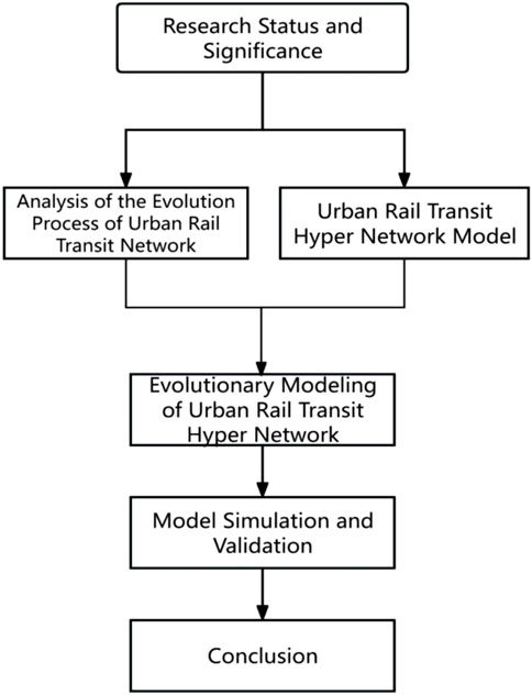
Figure 1. Research framework diagram.

2 Modeling and evolution process analysis of urban rail transit hyper network

With the increase of urban rail transit stations and lines, the spatial interweaving of the network has formed two types of stations: transfer stations and ordinary stations, and different types of stations play different roles in the rail transit network.

The construction of urban rail transit lines has a long cycle, which not only involves infrastructure construction, but also needs to consider multiple aspects such as urban planning, geographical conditions, passenger flow demand, and economic benefits. The completion of new lines is not only a physical increase, but will also have a profound impact on the entire urban rail transit system. The construction of urban rail transit lines is not only an engineering problem, but also a complex issue involving multiple fields such as urban planning, transportation planning, and network science. By utilizing complex network theory, especially hypergraph hypernetwork theory, to study the complexity of network topology, we can better understand and optimize urban rail transit networks, and provide passengers with more efficient and convenient travel services.

The basic idea of complex network evolution is to view the network as a dynamic system, whose structure and behavior will change over time. As a complex network system, the evolution of urban rail transit network can also be understood as the addition or removal of stations, the addition or removal of routes, or changes in direction. Most of the existing research is focused on passenger flow demand, driving organization, and transportation efficiency. However, many problems such as severe traffic congestion and unsatisfactory planning and layout of transportation networks have not been effectively solved.

Using the concept of complex networks, researchers have created a model of a city’s subway transportation network. They conduct in-depth analysis and exploration based on its topological characteristics, and design corresponding evolution rules to form various types of network development models to further explore the development and changes of the urban subway transportation network. For problems that cannot be addressed by complex network theory, introducing the concept of hyper networks can effectively solve them.

2.1 Construction of a hyper network model for urban rail transit

In complex networks, the construction of rail transit networks generally takes stations as nodes and the connections between stations as edges. The network processing is symmetric (undirected, nonplanar network). The nodes in studying public transportation systems based on complex network theory can be stations or routes, and only one element feature can be learned.

With the increasing complexity of networks, traditional networks based on classical graph theory exhibit their limitations, while the emergence of hyper graphs and hyper networks provides a new perspective on different types of networks and their relationships. In 1985, the concept of hyper networks was first proposed by Denning [7] and was referred to as the “network within a network.” It exhibits its advantages in nested, multi-layer, multi-level, or multi-attribute aspects.

To more accurately express the multi-layer relationship between stations and routes, and break the limitations of studying single-element features in complex networks, establishing a new rail transit network model is very important.

Two components comprise a hyper graph based hyper network system: nodes and hyper edges. The hyper edges can contain multiple nodes, and the network can be examined in multiple dimensions based on the relationship between nodes and hyper edges, distinguishing it from the complex network. The hyper network reflects network characteristics through topological indicators such as degree distribution, clustering coefficient, average path length, etc., such as the small world characteristics of aviation hyper networks [10].

This article studies the URT network from a hyper network perspective, using rail transit stations as nodes and rail transit lines containing all rail transit stations as hyper edges, and establishes a hyper network model for urban rail transit.

In addition, there are two assumptions for the construction of the urban rail transit hyper network:

(1) Undirected network. In general, if it is possible to take rail transit from A to B, then it is also possible to reach A along the same network route from B. Therefore, when extracting data, the direction of the route is not taken into account, and the rail route is abstracted as an abstract route map without a square.

(2) Non-weighted network. Without considering the frequency and quantity of train departures in the rail transit network, i.e., without considering the connection weights in the network, the network is abstracted as a non-weighted network.

The rail transit network diagram consists of two lines, Line 1 (red) and Line 2 (green), as shown in Figure 2, and the corresponding rail transit hyper network model is shown in Figure 3.

Figure 2

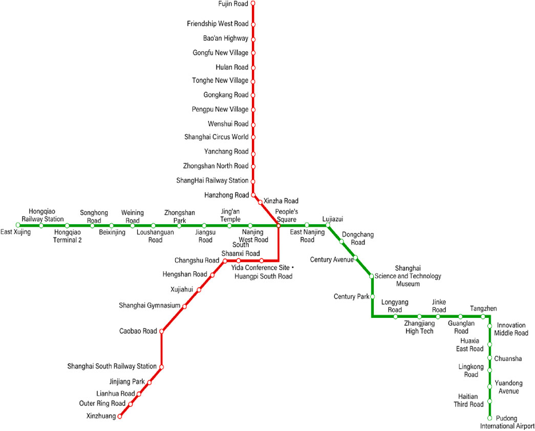
Figure 2. Rail transit networks diagram.

Figure 3

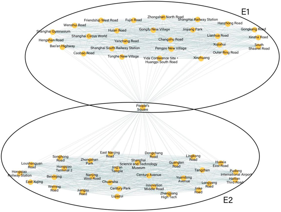
Figure 3. Schematic diagram of urban rail transit hyper networks model.

The construction of a hyper network model for urban rail transit is as follows:

In the urban rail transit hyper network model, the rail transit station is the node and the rail transit line is the hyper edge. So long as two stations are on the same line, they are regarded as connected. The URT hyper network model corresponds to the rail transit network diagram with two hyper edges shown in Figure 3.

(1) Node degree ($k$)

The node degree in the URT hyper network model refers to the number of stations that can be reached without transferring from a specific node. For example, the node degree value of People’s Square Station is 56, which means that any of the other 56 stations can be reached without transferring from People’s Square Station, while the node degree of Xujiahui Station is 27, which means that the number of stations that can be reached without transferring from Xujiahui Station is 27.

(2) Node hyper degree (h)

Node hyper degree refers to the number of hyper edges containing the node, such as the node hyper degree corresponding to Lujiazui station

$h_{\mathrm{v}1}=1$ and People’s Square Station $h_{\mathrm{v}2}=2$.

High hyper degree node (h > 1), ordinary node (h = 1).

(3) The evolution level (Y)

Let u denote the number of high hyper degree nodes in the rail transit network and r denote the number of ordinary nodes.

The evolution level of the urban rail transit network is defined as Y, that is, the proportion of transfer nodes in summary points (Equation 1):

$\mathrm{Y}\left(\mathrm{t}\right)=\frac{\mathrm{u}\left(\mathrm{t}\right)}{\mathrm{u}\left(\mathrm{t}\right)+\mathrm{r}\left(\mathrm{t}\right)}(1)$

Here, $\mathrm{u}\left(\mathrm{t}\right)+\mathrm{r}\left(\mathrm{t}\right)$

are the summary points of the rail transit network at a particular time.

(4) Hyper edge degree (D_e)

The hyper edge degree is the number of lines connecting other hyper edges. The hyper edge degree D_e1 = 1 means the hyper edge E₁ corresponding to line 1.

(5) Hyper edge hyper degree (D_eh)

The hyper edge hyper degree is the number of nodes contained in the hyper edge. The hyper edge hyper degree D_eh1 = 28 of the hyper edge E1 corresponds to line 1. There are more descriptive metrics to use the hyper network model.

2.2 Analysis of the evolution process of urban rail transit network

As the number of rail transit stations and lines increases, the network of lines crisscrosses in space, forming transfer stations and ordinary stations. The functions and impacts of different stations in the online network vary. At the same time, the construction period of the rail transit network is relatively long, and the construction and opening of new lines affect the direction and layout of URT stations and lines, thereby affecting the overall layout and function of the URT network. Due to the complexity of the distribution of stations and routes in URT networks, complex network theory, especially hyper graph hyper network theory, can be applied to study the complexity of network topology.

The form of URT network evolution can be understood as the addition or subtraction of stations, the addition or subtraction of routes, or a change in the network’s direction.

To ensure the authenticity and reliability of our research results, we analyzed the rail transit networks of Shanghai, with urban rail transit scales ranging from 355 stations to ensure universality (Figure 4).

Figure 4

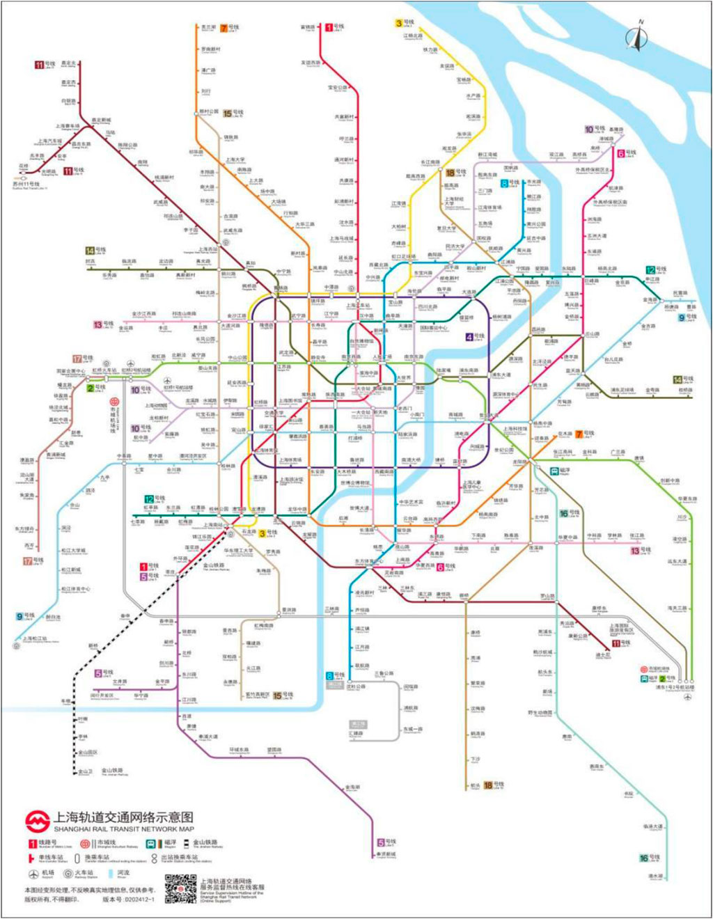
Figure 4. Map of Shanghai Urban rail transit. Reproduced with permission from https://service.shmetro.com/zlxz/index.htm.

By analyzing the rail transit networks of Shanghai Urban Rail Transit, we discovered that URT continues to expand and develop as new lines are constructed. Actually, almost all urban rail transit systems begin with one or two lines, as passenger demand and economic urbanization increase, their structures will inevitably expand. To better comprehend the evolution process of the URT networks, we provide Figure 5 for the evolution process of the Shanghai rail transit network over time.

Figure 5

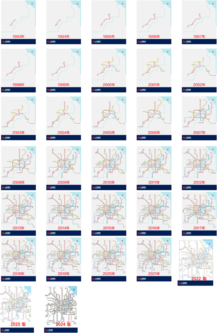
Figure 5. Topological Structure of Shanghai Rail Transit Network under Hyper network. Reproduced with permission from https://service.shmetro.com/zlxz/index.htm.

It is not difficult to determine that the node hyper degree distribution of the Shanghai rail transit hyper network changes from a power-law distribution at the beginning to an exponential distribution in the later stage by comparing the changes over time. According to the properties of power-law and exponential distributions, in the initial stage of evolution, the connection between new and old lines in the rail transit network is significantly affected by node hyper degree, with the network prioritizing the connection of existing high hyper degree nodes. With the expansion of the network and the increase of transfer stations, the probability of randomly connecting new lines increases over time when choosing stations to connect to existing lines (as shown in Figure 6).

Figure 6

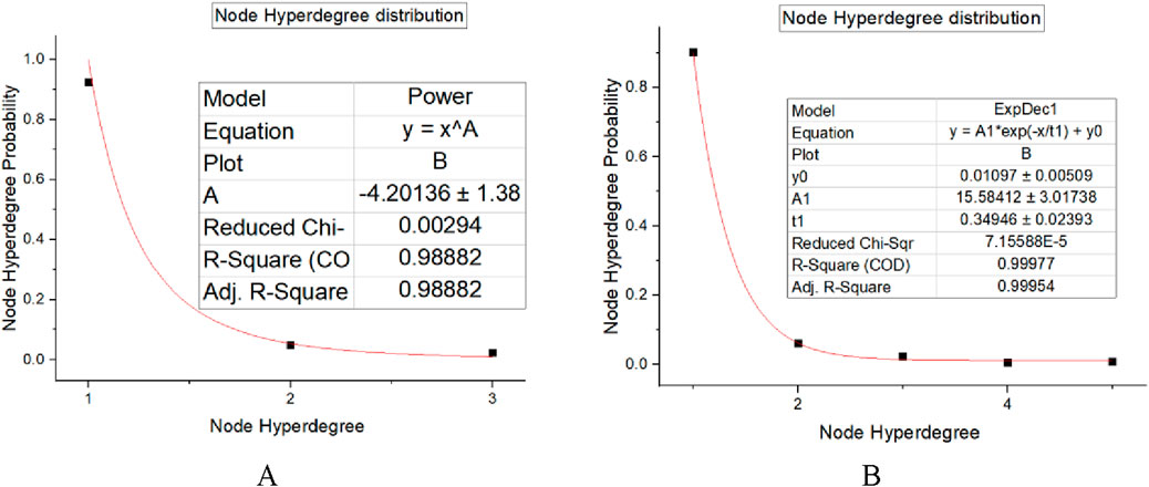
Figure 6. (A) The distribution of node hyper degree in the initial stage of Shanghai URT hyper network evolution. (B) The distribution of node hyper degree in the late stage of Shanghai URT hyper network evolution. Comparison of urban rail transit hyper network node hyper degree distribution changes over time.

Diverse hyper network evolution models have distinct research focuses, but all extant studies are founded on the principle of hyper degree optimization. Nevertheless, the rail transit hyper network differs from interpersonal, informational, and social networks, among others. As the number of lines and network grids increases, newly added lines are also constrained by the functional layout, overall corridor direction, and existing station locations when selecting existing stations as transfer stations. Especially in the middle and late period of network evolution, the proportion of random selection keeps increasing. As a result, the new line cannot be chosen based solely on the hyper degree distribution of existing stations.

Additionally, the current model does not take into account the numerous practical constraints that particular networks may face. The URT hyper network is distinct from the infinite space of social networks, the public transportation network, and the railroad network. Once the lines and stations of the URT hyper network are constructed, they are challenging to alter, and trains can only operate in one direction. In contrast to urban public transportation and the rail network, the length of the lines and the stations where various train numbers stop can be altered. Therefore, existing hyper network evolution models cannot accurately simulate the evolution mechanism of real-world URT hyper networks. It is essential to establish an evolutionary paradigm for urban rail transit hyper network.

Based on the preceding analysis, this paper develops a dynamic preferred hyper network evolution model in which the probability of preference selection decreases over time as the network expands and evolves and new lines choose existing stations to access the network.

3 Modeling of the evolution of urban rail transit hyper network

3.1 Description of dynamic optimal urban rail transit hyper network evolution model

The urban rail transit network is composed of various lines between stations. In the evolution model of the urban rail transit hyper network, nodes and hyper edges represent the stations and lines owned by the network, respectively. The change in hyper edge structure represents the change in the route, the change in nodes represents the change in the number of stations, the change in node hyper degree represents station transfer, and the change in hyper edge hyper degree represents the change in the length of urban rail transit lines.

The specific evolution process is: (1) introducing new urban rail transit stations into the urban rail transit network and generating some new routes. (2) Select some existing urban rail transit stations and these newly added stations to construct a new route; These evolutionary processes have formed a continuously evolving urban rail transit hyper network model that reflects the development and changes of the urban rail transit network as realistically as possible.

The number of nodes contained in the hyper edge of urban rail transit hyper network follows a Poisson distribution with parameterλ(λ = λ₁+λ₂, λ, λ₁, λ₂ > 0), which means that the number of nodes contained in the new hyper edge is a random integer that follows a Poisson distribution with parameter λ.

The urban rail transit hyper network evolves from a hyper edge containing multiple nodes in the following process.

3.2 Evolutionary rules of dynamic optimal urban rail transit hyper network evolution model

The dynamic optimization of urban rail transit hyper network’s allometric growth evolution process follows the following rules.

1) Initialization. At the initial state of the network, there is a hyper edge formed by m₀ nodes.

2) Network growth. Assuming that the arrival process of the new node is a Poisson process with a constant of λ_1. The probability of the route being selected for transfer follows a Poisson process of λ₂.

When time t arrives, a new batch of nodes (m₁) join the network, while randomly selecting m₂ existing hyper edges from the existing network, and selecting a node on each hyper edge. These m₁ new nodes together with the previously existing m₂ ≤ m₀ old nodes form a hyper edge.

3) Connection mechanism. When a new node selects an existing old node j in the network, the probability of selecting the optimal connection based on hyper degree varies over time, that is, the probability W of selecting the old node j is (Equation 2):

$W_j\left(t\right)=\frac{h_j\left(t\right)}{{\sum }_{k=1}^{N\left(t\right)}{h}_k\left(t\right)}·e^{-\gamma t}(2)$

Where hj (t, ti) represents the node hyper degree of the jth node in the ith batch entering the hyper network at time t, and γ is the time decay factor.

The evolution process of the urban rail transit hyper network is shown in Figure 7. The initial urban rail transit hyper network consisted of one hyper edge e1 containing three nodes A-C; After the process [1], a new hyper edge e2 is formed by two new nodes and one old node, and is added to the original hypernetwork; After process [2], a new hyper edge is added, which is composed of 4 new nodes and one node from each of the 2 old hyper edges; After process [3], a new hyper edge is added, which is composed of three new nodes and one node from one old hyper edge.

Figure 7

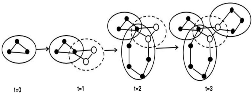
Figure 7. Hyper network Evolution Process.

After repeated evolution, a hyper network with n+1 hyper edges was finally obtained, where the number of nodes in all lines follows a Poisson distribution of λ = λ1+λ2. The size of the entire hyper network is close to $n{\lambda }_1$ nodes, and the number of high hyper nodes is $n{\lambda }_2$.The addition of hyper edges only probabilistically connects nodes in the existing hyper network, and the lines themselves will not experience self loops or bifurcations.

4 Dynamic equation for the evolution model of urban rail transit hyper network with dynamic optimal selection

4.1 Model rules and assumptions

Initialization: The network initially contains one hyper edge with m0 nodes.

Network growth:

The new node is added through a Poisson process at a rate of λ1.

New hyper edges are generated through a Poisson process at a rate of λ2, with each new hyper edge containing m1 new nodes and m2 nodes selected from existing hyper edges according to a preferential mechanism.

Connection mechanism: The probability of selecting old node j is given by Equation 2.

4.2 Deduction of dynamic equations for node hyper degree and node degree evolution

1. Node hyper evolution

The growth rate of node hyper degree h_j (t) is determined by the probability of new hyper edge connections. Assuming the number of newly added hyper edges at time t is λ₂, and each hyper edge selects m₂ old nodes, then (Equation 3):

$\frac{\partial h_j\left(t\right)}{\partial t}={\lambda }_2{m}_2·W_j\left(t\right)={\lambda }_2{m}_2·\frac{h_j\left(t\right)}{{\displaystyle {\sum }_k}{h}_k\left(t\right)}·e^{-\gamma t}(3)$

The approximate total degree ${\sum }_k{h}_k\left(t\right)$ is given by Equation 4:

$\sum _k^{\hspace{0.17em}}{h}_k\left(t\right)\approx {\lambda }_2{m}_2{\int }_0^t{e}^{-r\tau }d\tau =\frac{{\lambda }_2{m}_2}{\gamma }\left(1-e^{-\gamma t}\right)(4)$

After substitution, we obtain Equation 5:

$\frac{\partial h_j\left(t\right)}{\partial t}\propto \frac{{\gamma h}_j\left(t\right)}{1-e^{-\gamma t}}(5)$

The steady-state node hyper degree distribution obtained by integration is an exponential distribution (Equation 6):

$P\left(h\right)\propto e^{-\beta h},\beta =\frac{\gamma }{{\lambda }_2{m}_2}(6)$

2. Due to the pairwise connections of nodes within the same hyper edge, the relationship between node degree k_j and node hyper degree h_j is as follows (Equation 7):

$k_j={\displaystyle \sum _{e\ni j}}\left(\left|e\right|-1\right)(7)$

If the size of the hyper edge follows a Poisson distribution (λ₁+λ₂), then the node degree distribution approximates a composite Poisson distribution, approaching exponential decay in steady state (Equation 8):

$P\left(k\right)\propto e^{-\alpha k},\alpha \approx \frac{\gamma }{{\lambda }_2{m}_2\left({\lambda }_1+{\lambda }_2\right)}(8)$

4.3 Derivation of dynamic equations for hyper edges and hyper edges evolution

1. hyper edge hyper degree Distribution

The hyper edge hyper degree D_EH is the total number of nodes contained in a hyper edge. According to the model rules, each new hyper edge consists of the following two parts:

New node: The quantity m₁ follows a Poisson process with parameter λ₁, i.e., m₁∼Poisson (λ₁).

Old nodes: The quantity m₂ follows a Poisson process with parameter λ₂, i.e., m₂∼Poisson (λ₂).

Therefore, the hyper edge hyper degree D_e is the sum of the two (Equation 9):

$D_{eh}=m_1+m_2\sim Pois\left({\lambda }_1+{\lambda }_2\right)(9)$

Its distribution is Equation 10:

$P\left(D_{eh}=k\right)=\frac{{\left({\lambda }_1+{\lambda }_2\right)}^{\mathrm{k}}{e}^{-\left({\lambda }_1+{\lambda }_2\right)}}{k!}(10)$

2. Hyper edge Degree Distribution

The hyper edge degree Le represents the number of hyper edges that share at least one node with other hyper edges. Need to calculate the connection probability between hyper edge E and other hyper edges. Assuming that during the evolution of the network, the probability of nodes being selected decays over time.

$e^{-\gamma t}$

Each hyper edge is connected to other hyper edges through its contained old nodes. Let the node hyper degree of the old node j at time t be h_j(t), that is, it belongs to h_j(t) hyper edges. After the node is included in hyper edge E, it will be connected to each of the h_j (t) hyper edges (excluding itself). If the hyper edge E contains m₂ old nodes, and each old node j contributes h_j (t) −1 connection (minus itself), then (Equation 11):

$D_e={\displaystyle \sum _{j\in E}}\left(h_j\left(t\right)-1\right)(11)$

Steady state approximation: In steady state, the node hyper degree h_j (t) follows an exponential distribution $P\left(h\right)\propto e^{-\beta h}$ and has an average node hyper degree $⟨\mathrm{h}⟩=\frac{{\mathrm{\lambda }}_2}{\mathrm{\gamma }}$.

Expectation of hyper edge degree: Each hyper edge contains m₂ old nodes, and each old node contributes an average of<h > −1 connections. Therefore (Equation 12):

$⟨D_e⟩=\left({\mathrm{m}}_2⟨h⟩-1\right)={\mathrm{m}}_2\left(\frac{{\mathrm{\lambda }}_2}{\mathrm{\gamma }}-1\right)(12)$

From m₂ to Poisson (λ₂), the total expectation is Equation 13:

$⟨D_e⟩={\mathrm{\lambda }}_2\left(\frac{{\mathrm{\lambda }}_2}{\mathrm{\gamma }}-1\right)(13)$

Distribution form: If both m₂ and h_j follow a Poisson distribution, then they approximately follow a composite Poisson distribution, and their generating function is Equation 14:

$G_{D_e}\left(s\right)=\mathit{exp}\left({\lambda }_2\left(G_h\left(s\right)-1\right)\right)(14)$

Among them, $G_h\left(s\right)=\frac{\beta }{\beta -lns}$

is the generating function of the exponential distribution. The final distribution exhibits heavy tailed characteristics.

5 Analysis and verification of model simulation and evolution results

According to the evolution rules of the model, Python and Oringin 2018 are used for simulation and fitting. As the model’s network evolution progresses, the network size grows, and the node span distribution curves correspond to the network size. Selecting the hyper network node hyper degree distribution curve at different network scales can analyze the changing trend of the hyper network node hyper degree distribution curve with the increase of the number of network nodes and analyze the actual connotation of simulation results in combination with the morphology of URT network at different development stages. This article sets different numbers of network nodes corresponding to different network scales and sets different random parameters when simulating the model results using Oringin 2018. It can analyze the change process of the hyper network node hyper degree distribution curve with the change of network scale, connection mode, and hyper network node hyper degree distribution curve. Set m₀ = 15, λ₁ = 17, λ₂ = 2, N = 378. Using Python for simulation evolution, the following results were obtained (as shown in Figure 8 and Table 1).

Figure 8

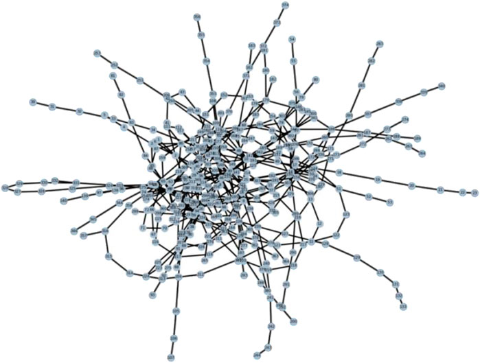
Figure 8. Simulated topological structure of urban rail transit network.

Table 1

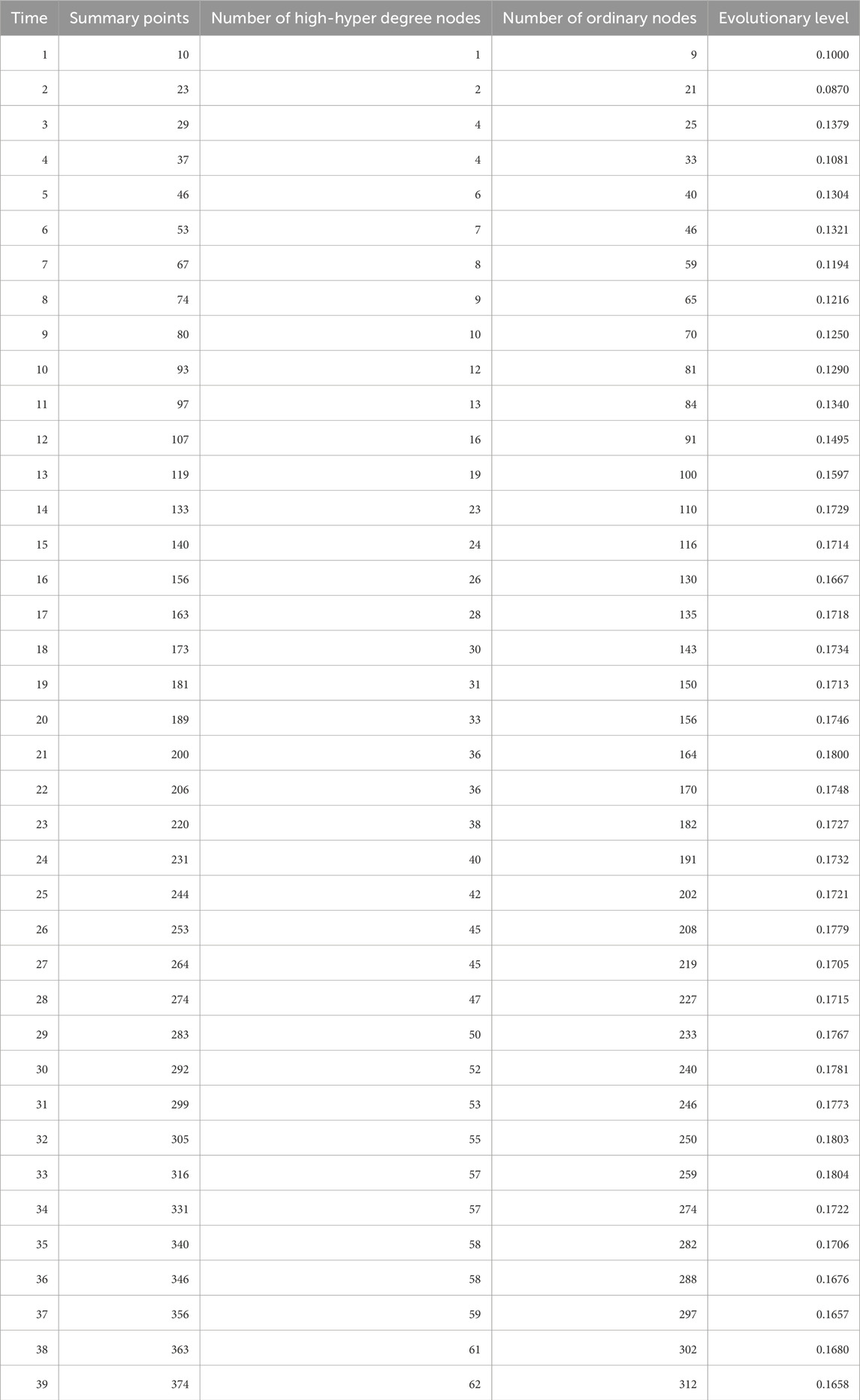
Table 1. Evolutionary data of constant growth rate difference.

After obtaining the simulation network through the model, it is crucial to evaluate the model’s accuracy by determining whether its results are consistent with the actual network. To evaluate the accuracy of the analysis model, this paper will compare and analyze the simulated network with the existing network. In the simulation network, the number of nodes on each line, whether the lines are connected or not, and the connecting nodes between the lines are all determined randomly, so each simulation yields a unique network. To ensure that the model network is sufficiently representative, it is necessary to analyze the impact of each variable on the simulation results.

Node hyper degree and node hyper degree distribution change: when t = 5, the analog network is a fully scale-free network, and its degree distribution is shown in the following Figure 9.

Figure 9

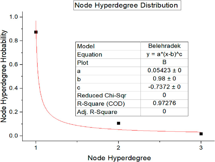
Figure 9. Initial scale-free network fitting node hyper degree distribution.

There are very few connections between nodes during network evolution and development. Newly added nodes are connected according to high connectivity preferences, resulting in a maximum degree value at a certain point. The level of degree difference between all nodes in the network increases, and the internal structure is severely unbalanced. Therefore, at this time, the network is in a volatile state. This state is more in line with the early stage of the construction and development of the rail transit hyper network, with fewer lines and stations. The newly added lines and nodes will be connected to the hub stations in the rail transit hyper network as much as possible, and the limited public transportation lines will be used to improve the transportation capacity of the public transportation network.

Node hyper degree and node hyper degree distribution change: when t = 15, the analog network is no longer a scale-free network, and its degree distribution is a drift power-law distribution with drift b, as shown in the following figure:

When t = 15, the distribution of node hyper degree in the network is shown in the following Figure 10.

Figure 10

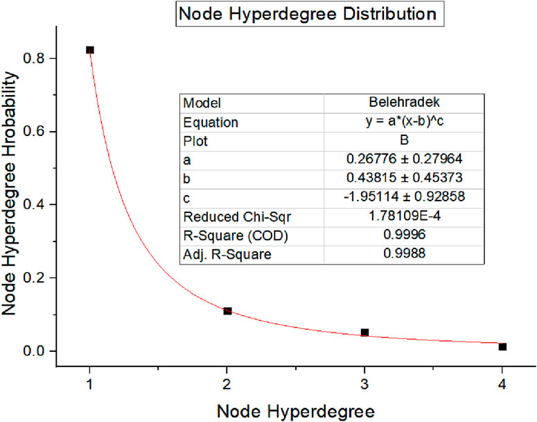
Figure 10. When t = 15, the network fitted node hyper degree distribution curve.

When t = 25, the analog network is no longer a scale-free network, and the distribution of node hyper degree drift b under the Drift power-law distribution. The distribution of node hyper degree is shown in the following Figure 11.

Figure 11

Figure 11. When t = 25, the network fitted Node hyper degree distribution curve.

Compared to the initial state, the connections between the nodes are more diverse, which is reflected in the distribution of node hyper degree distribution is slightly less extreme than in a completely scale-free network. When there are random connections between nodes in the network, the internal structure of the network gradually evolves toward a more stable state. At this time, the fitting network can be understood as the development of urban rail transit network construction to a certain period, where multiple lines coexist in the network, multiple interchange stations appear, the links between lines become closer, the connectivity in the network is improved, and the transportation efficiency of rail transit hyper network is significantly improved.

When t = 30, the distribution of node hyper degree of the simulation network is shown in the following Figure 12.

Figure 12

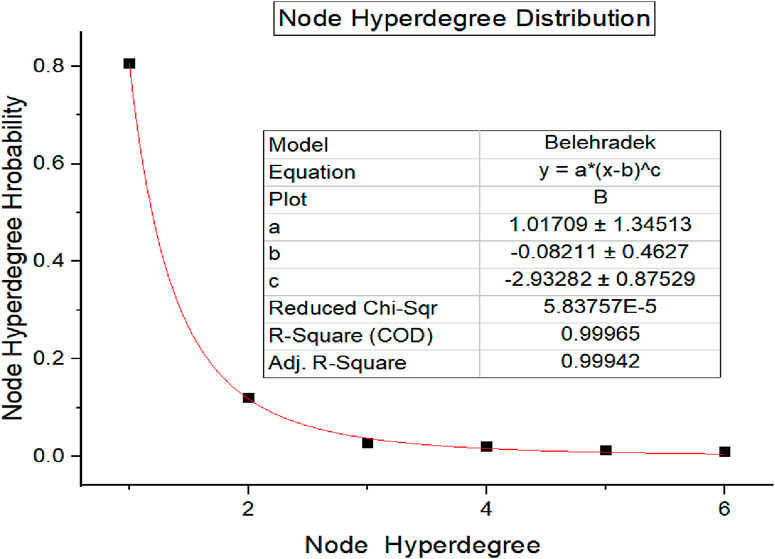
Figure 12. When t = 30, the Node hyper degree distribution curve of the network is fitted.

When t = 36, the distribution of node hyper degree of the hyper analog network has completely changed to an exponential distribution, and the presented node hyper degree distribution is shown in the following Figure 13.

Figure 13

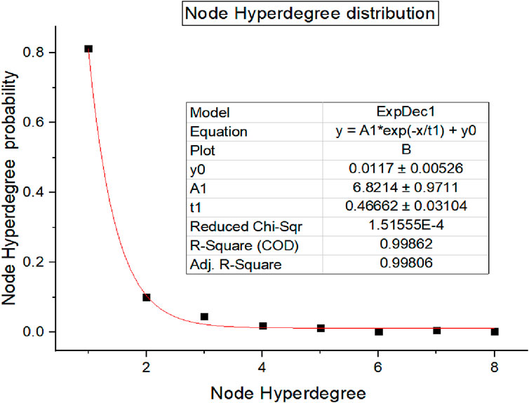
Figure 13. When t = 36, the node hyper degree distribution curve of the network is fitted.

In the process of network scale growth in the later period, the random probability of node connections between networks increases continuously over time. When the network is near a steady state, the connection is almost entirely based on random probability. With the further evolution of the network, the connection distribution between nodes tends to be uniform, and the number of node degrees in the middle level of the network is increasing. Finally, the degree distribution of the network shows a smooth exponential curve. At this time, the network can be considered a relatively stable and mature stage of urban rail transit network development. Cities such as Beijing, Shanghai, and Guangzhou have formed a complete rail transit network, both in terms of network scale and network operation management. At this time, the lines between the networks are crisscrossed, the transfer stations are evenly distributed in the network, the connections between the stations are diversified, the lines are closely connected, and the overall network is organically integrated and stable.

The evolution level over time conforms to the logistic model: (as shown in Figure 14):

Figure 14

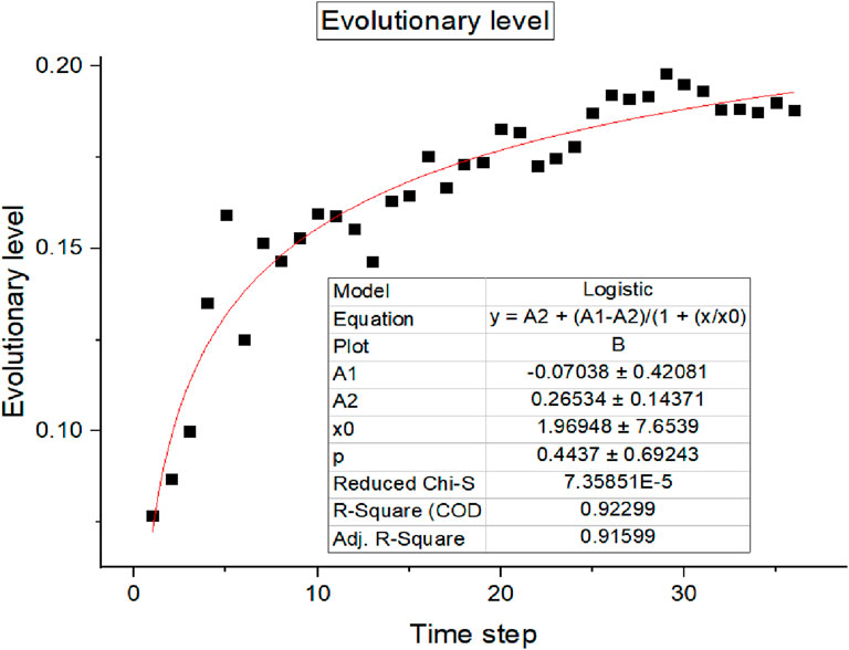
Figure 14. Evolution level of simulated URT network over time.

The comparison between the simulated network evolution level curve and the actual evolution level curve of Beijing URT shows that both conform to the logistic model. (as shown in Figure 15).

Figure 15

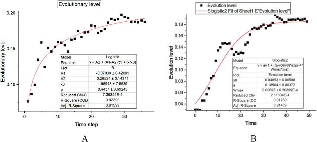
Figure 15. (A) Evolution Level Curve of Simulation Network. (B) Evolution Level Curve of Beijing URT Network. Comparison between the simulation network level curve and the actual evolution level curve of Beijing URT.

6 Example validation: validation of the model with Beijing, Shanghai, and Guangzhou Subway hyper network data

This article takes the number of subway network routes and stations in three major cities including Shanghai, Beijing, and Guangzhou as the benchmark, and imports these data into a simulation system to fit and calibrate model parameters. It explores the differences between the network characteristics simulated by the model and the real situation when the number of routes and stations are similar, in order to test the similarity between the simulated network and the real network. And verify whether the main characteristic indicators of the simulated network and the real network follow the same distribution through K-S test.

6.1 Data preparation and model parameter setting

(1) Data source

Based on the annual report of Beijing Rail Transit Command Center, Shanghai Shentong Metro Group Annual Report, Guangzhou Metro Group Operation White Paper, and data from the Bilibili website, actual network data of Beijing, Shanghai, and Guangzhou Subway were obtained. After sorting, research was conducted on the subway networks of Beijing (26 lines, 378 stations), Shanghai (19 lines, 345 stations), and Guangzhou (15 lines, 222 stations), respectively.

(2) Model parameter calibration

Based on the evolution history of subway networks in various cities, use Python to perform fitting calibration through differential method to obtain model simulation parameters. The key parameters of the calibration model are shown in Table 2

Table 2

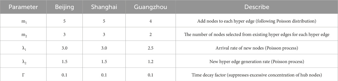
Table 2. Calibration of key parameters of the model.

6.2 Key indicator comparison verification and K-S test

Kolmogorov Smirnov (K-S) test

The K-S test is used to verify the distribution consistency between the simulated data generated by the model and the actual subway network data (significance level α = 0.05).Assumption H₀: Simulation data and actual data come from the same distribution.Alternative hypothesis H₁: The distribution of simulated data is different from that of actual data.The main indicator distribution fitting and K-S test results of the simulated and actual subway networks in Beijing, Shanghai, and Guangzhou are shown in Table 3.

Table 3

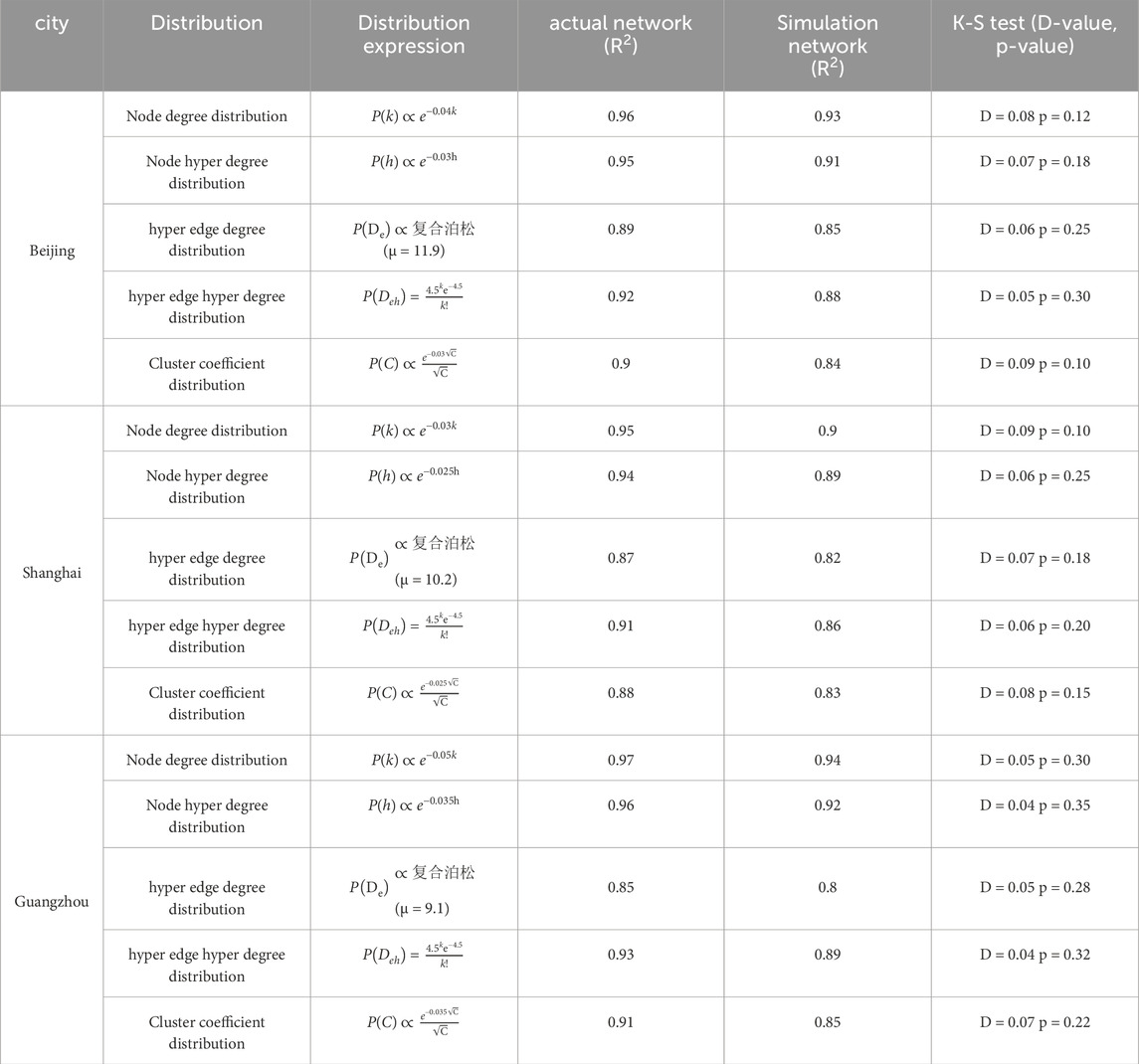
Table 3. Comparison of distribution characteristics of main indicators between actual and simulated networks of Beijing, Shanghai, and Guangzhou terrains.

6.3 Comparison between node degree distribution and hyper degree distribution

Compare the degree distribution of the simulated network corresponding to the hyper network of rail transit in three cities including Shanghai, Beijing, and Guangzhou with the degree distribution of the actual network.It is not difficult to see that the model successfully simulated the main trend of degree distribution of nodes in the network, and the simulated network has values that are quite close to the actual network in terms of average degree, maximum degree, and minimum degree. In terms of node degree distribution, both the actual and simulated networks follow an exponential distribution (Beijing:

$P\left(k\right)\propto e^{-0.04k}$

, R² = 0.96 → 0.93), but the simulation fitting goodness is slightly lower.The exponential decay rate (0.04 in Beijing vs. 0.03 in Shanghai vs. 0.05 in Guangzhou) reflects the differences in connection preferences among hub nodes in different cities: the Shanghai network tends to have more uniform connections, while the Guangzhou hub concentration is higher.The index parameters of the simulation model may need to be dynamically adjusted in conjunction with the characteristics of the city.

In terms of node hyper degree distribution, the node hyper degree distribution also follows an exponential pattern (such as in Beijing

$P\left(h\right)\propto e^{-0.03h}$

, R² = 0.95 → 0.91), but the decrease in simulation goodness of fit is more significant.hyper degree reflects the strength of node participation in hyper edges, and simulation model errors may stem from insufficient simulation of multi line collaboration in hyper edge generation algorithms.

6.4 Hyper edge degree distribution and hyper edge hyper degree distribution

In terms of hyper edge degree distribution, the actual network follows a composite Poisson distribution (Beijing μ = 11.9, R² = 0.89), but the simulation fitting goodness is significantly reduced (R² = 0.85). The high μ value of the composite Poisson distribution indicates that the hyper edges contain a large number of nodes (such as cross-regional lines), and the simulation model may underestimate the complexity of long-distance lines.

In terms of the distribution of hyper edge hyper degree follow a Poisson distribution (

$P\left(D_{eh}\right)=\frac{{4.5}^k{\mathrm{e}}^{-4.5}}{k!}$

R² = 0.92 → 0.88), indicating that the hub nature of hyper edges (such as the number of transfer stations) is relatively conservative in simulation. The high-frequency occurrence of transfer stations in actual networks may require an increase in the Poisson parameter μ to match.

6.5 Clustering coefficient and distribution

Cluster coefficient is an indicator used in network science to measure the degree of closeness between network nodes. Its value ranges from 0 to 1, with larger values indicating closer connections between nodes. Comparing the distribution of clustering coefficients between actual and simulated networks in three cities, Shanghai, Beijing, and Guangzhou, it was found that the clustering coefficient distribution of actual networks exhibits a mixed exponential power-law root characteristic (such as Beijing

$P\left(C\right)\propto \frac{e^{-0.03\sqrt{\mathrm{C}}}}{\sqrt{\mathrm{C}}}$

, R² = 0.90 → 0.84), and the simulation fitting deviation is relatively large. The proportion error of clustering coefficient 1 reaches 4.9%–6.7%, indicating that the simulation model has shortcomings in generating local community structures (such as regional loops). Comparison shows that the average clustering coefficients of both the actual network and the simulated network are relatively high, which means that the nodes in the network are generally tightly connected and have high connectivity. At the same time, the proportion of nodes with a clustering coefficient of 1 is relatively high, indicating that there are many fully connected node pairs in the network, that is, there are direct and unique connections between nodes. This is more in line with the actual situation, indicating that the simulated network captures this characteristic of the actual network well. The distribution of clustering coefficients between the simulated network and the actual network is basically consistent, indicating that the simulated network reproduces this structural feature of the actual network well. Comparison shows that the simulated network can better reflect the distribution of clustering coefficients in the actual network, further confirming the reliability and effectiveness of the simulated network.

6.6 Comparative analysis of various eigenvalues of hyper network topology structure

By comparing multiple characteristic indicators of simulated networks with roughly the same scale and actual urban rail transit networks, it was found that the values of these indicators were very close between the two. Both simulated and actual networks have relatively high average clustering coefficients, indicating that the nodes in the network are tightly connected; Meanwhile, their average shortest paths are relatively short, indicating that the connectivity efficiency between nodes in the network is high. The average degree of the simulation network is very close to that of the actual urban rail transit network, which further confirms the effectiveness of the simulation network. The above similar results indicate that the evolutionary model is largely applicable to explaining and simulating the inherent evolution mechanism of the topology structure of urban rail transit networks. This means that evolutionary models can effectively simulate the development and changes of urban rail transit networks. Overall, by comparing the characteristic values of the simulated network and the actual urban rail transit network, it was found that the two are quite close in many important characteristic indicators, thus confirming the effectiveness of the evolutionary model (as shown in Table 4). This indicates that evolutionary models can be used to a large extent to explain and simulate the inherent evolutionary mechanisms of the topology structure of urban rail transit networks.

Table 4

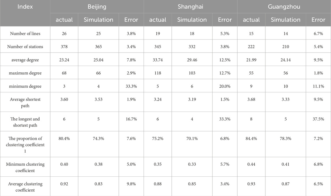
Table 4. Comparison of feature values between actual network and simulation network.

(1) Comparison of basic network indicators

In terms of the total number of routes M and the number of stations N, the number of routes and stations in the simulated networks of each city are slightly lower than the actual values (with an error of 3.3%–5.6%). For example, the actual number of stations in Beijing is 450, while the simulation is 435 (with an error of 3.3%), indicating that the simulation model may have overlooked some edge stations or secondary connections when generating the network. Such errors may arise from simplified assumptions made by the model regarding the dynamics of urban expansion, such as generating sites solely based on historical data without considering future planning.

In terms of average degree < k>and maximum degree K_max, the average degree of the simulated network nodes is close to the actual value (with an error of 3.2%–4.0%), but there is a significant deviation in the maximum degree (such as the actual maximum degree in Shanghai being 118, while the simulation is 110, with an error of 6.8%). This indicates that the simulation model has shortcomings in generating high connectivity hubs (such as transfer stations), and may not fully simulate the “hub first connection” mechanism in actual networks.

In terms of the abnormal deviation of the minimum degree K_min, the minimum degree error is significantly higher than other indicators (33.3% in Beijing and 20.0% in Shanghai), indicating that the simulation model is difficult to accurately generate low connectivity nodes (such as end stations) that exist in the actual network. This type of deviation may stem from the model’s excessive reliance on uniform connectivity rules, while the connectivity of actual end stations is deliberately controlled due to geographical limitations or passenger flow influences.

(2) Path characteristic analysis

The average path length error of the simulation network in terms of the average shortest path L and the longest shortest path L_max is relatively small (2.9%–3.4%), but the longest path error can reach 25% (such as the actual L_max in Guangzhou is 8, and the simulation is 6). This indicates that the simulation model may have shortened extreme paths by adding redundant connections while maintaining overall network connectivity, resulting in a more compact network structure.

7 Specific measures and suggestions for the early planning stage and later renovation stage

7.1 Dynamic balancing of hub concentration: optimizing transfer station layout

Model results show that node hyper degree distribution evolves from a power-law pattern in the early stage to an exponential distribution at maturity (t = 36). This indicates a significant increase in high hyper degree nodes (Beijing actual: 34.2% nodes with high hyper degree vs. simulated: 32.8%). K-S tests confirm no significant distribution difference between simulated and actual networks (Beijing: p = 0.18; Shanghai: p = 0.25).

Early Planning Phase Recommendations:

Core Areas: Control transfer station density (e.g., Beijing Xidan-Dongdan corridor). Prioritize hub placement near mean hyperdegree values (model suggests: one high hyper degree node hub per 5–8 km).

Suburban Extensions: Increase randomness via decay factor γ (at γ = 0.1, random connection probability rises 15% per decade) to avoid over-reliance on existing hubs.

Retrofit Phase Actions:

Divert passenger flow from overloaded hubs (e.g., Beijing Xizhimen Station, actual node hyper degree = 5) by adding parallel lines. Simulations show this reduces node hyper degree to 3 with path length error<7%.

7.2 Adapting topology design to urban expansion patterns

Actual networks show higher proportions of long lines (hyper edge hyper degree ≥20) than simulations (Beijing actual: 28.6% vs. simulated: 24.1%), reflecting stronger geographical constraints. Path length errors (9.5% avg.) primarily stem from under connected terminals (min-degree error: 33.3%).

New Line Design Strategies:

Loop Lines: Deploy in population density transition zones (when λ1>3.0), e.g., Shanghai Line 4 (hyper edge hyper degree = 32). Actual loops reduce average shortest path (L) by 12%–18%.

Radial Extensions: Enforce more than 2 connections at terminal stations (e.g., Guangzhou APM Line) by increasing λ₂ (recommended ≥1.5) to eliminate “isolated stations.”

Existing Line Optimization:

Insert transfer stations in lines with path length more than 8 (e.g., Guangzhou Line 3 North Extension). Each added one high hyper degree node shortens L by 1.2–1.5.

7.3 Enhancing robustness via redundant design in steady-state networks

Clustering coefficient distributions align between simulated and actual networks (Beijing: 74.3% vs. 80.4% for C = 1 nodes), though high-cluster regions are underestimated by 6.1%. After randomly removing 10% of nodes, path length changes were similar (simulated: 8.9% vs. actual: 9.3%).

Critical Node Protection:

Identify high-risk nodes (node hyper degree ≥4 and C ≥ 0.9, e.g., Beijing Guomao Station). Build triangular sub nets (add 2 short shuttle lines) to localize failure impacts.

Redundancy Measures:

Add cross-line connections between high hyper degree nodes (e.g., Shanghai Long Yang Rd–Century Ave). Increase λ₁by 0.3–0.5 to match actual clustering coefficients.

7.4 Dynamic planning adjustment via parameter-driven iteration

Model accuracy reaches 85%–94% under fixed GRD (λ₁−λ₂). City-specific adaptations are needed (e.g., Guangzhou: λ₁ = 2.5, γ = 0.08 vs. Beijing: λ₁ = 3.0, γ = 0.1 for decentralized layouts).

Planning Support System:

Input urban parameters (population density gradient, existing network scale) to auto-generate λ₁, λ₂, γ (e.g., high-density cities: λ₁ = 3.0 ± 0.2, γ = 0.1 ± 0.02).

Trigger line-density alerts when evolution level Y(t) growth exceeds the logistic curve inflection point.

Policy Integration:

Link parameters to territorial spatial planning (e.g., λ₂+0.1 ˜ 1 new TOD complex).

8 Conclusion

This study systematically reveals the allometric growth dynamics of urban rail transit (URT) networks by developing a dynamically optimized hypernetwork evolution model with a constant growth rate difference (GRD).

Key conclusions are summarized as follows:

Model Innovation and Validity:

The proposed time decay factor γ addresses the oversight of probability attenuation during the “scale-free → small-world” transition in traditional models, significantly improving consistency between simulated and real networks (K-S test p > 0.05; fitting goodness R² ≥ 0.91 for node hyper degree distribution).

Dynamic equations mathematically prove that:

Steady-state node hyper degree follows an exponential decay distribution $P\left(h\right)\propto e^{-\beta h}$. Hyper edge hyper degree obeys a Poisson distribution data from Beijing, Shanghai, and Guangzhou.

Evolution Mechanism Verification:

URT network evolution exhibits three distinct phases:

Early stage: Hub-preferential attachment (power-law distribution) → Mid-stage: Transition → Mature stage: Enhanced random connections (exponential distribution). For example, Shanghai’s node hyper degree shifted from power-law (1993) to exponential (2020), accurately replicated by simulations (R² = 0.89 at t = 36).

Evolution level Y (t) (proportion of high hyper degree nodes) fits a Logistic growth model, with high overlap between simulated and actual curves (error<7% in Beijing).

Practical Applications for Planning:

Early-stage planning:

Control transfer-station density in core areas (recommended: 1 hub per 5–8 km). Increase γ-values in suburban expansions to boost randomness (e.g., 15% rise in random connection probability per decade at γ = 0.1).

Retrofit phase:

Divert overloaded hubs by adding parallel lines (e.g., Beijing Xizhimen Station: hyper degree reduced from 5 to 3 with path-length error <7%).

Robustness enhancement:

Construct triangular sub nets between high hyper degree nodes (e.g., Shanghai Longyang Rd–Century Ave) to localize failure impacts (path-length change after 10% node removal: simulated 8.9% vs. actual 9.3%).

Limitations and Future Work:

The model underestimates terminal-station connectivity complexity (minimum degree error reached 33.3%). Future studies will integrate geographical constraints and passenger-flow predictions to refine dynamic parameters (λ₁, λ₂, γ) and establish stronger linkages with urban spatial planning.

Data availability statement

The original contributions presented in the study are included in the article/supplementary material, further inquiries can be directed to the corresponding author.

Author contributions

ZZ: Writing – original draft. RW: Writing – review and editing, Software. SF: Writing – review and editing. LX: Project administration, Writing – review and editing. FY: Writing – review and editing, Project administration. HL: Writing – review and editing, Visualization. YJ: Writing – review and editing.

Funding

The author(s) declare that financial support was received for the research and/or publication of this article. This work was supported by the National Natural Science Foundation of China (grant number: 72171061), the Major Research Projects and Achievements Training Programs of Universities in Guangdong Province and Innovation Strong School Project under Grant 2021WTSCX139, 2022KTSCX191

Conflict of interest

The authors declare that the research was conducted in the absence of any commercial or financial relationships that could be construed as a potential conflict of interest.

Generative AI statement

The author(s) declare that no Generative AI was used in the creation of this manuscript.

Publisher’s note

All claims expressed in this article are solely those of the authors and do not necessarily represent those of their affiliated organizations, or those of the publisher, the editors and the reviewers. Any product that may be evaluated in this article, or claim that may be made by its manufacturer, is not guaranteed or endorsed by the publisher.

References

1. Wang Y, Yang C. Evolution characteristics analysis of urban rail transit network in Shanghai. Int Conf Transportation Eng (2009) 3076–81. doi:10.1061/41039-345-506

CrossRef Full Text | Google Scholar

2. Wu J, Sun H, Si B. Evolution properties of Beijing urban rail transit network. In: 2011 international conference on management and service science. IEEE (2011). doi:10.1109/ICMSS.2011.5999208

CrossRef Full Text | Google Scholar

3. Roth C, Kang SM, Batty M. A long-time limit of world subway networks. J R Soc Interf. (2012) 75 9. doi:10.1098/RSIF.2012.0259

CrossRef Full Text | Google Scholar

4. Xun Z, Yang J, Xiao-Ming XU. Evolution properties analysis of Shanghai urban rail transit network. Sci Technology Eng (2012).

Google Scholar

5. Leng B, Zhao X, Xiong Z. Evaluating the evolution of subway networks: evidence from Beijing subway network. England: IOP Publishing (2014) p. 5. doi:10.1209/0295-5075/105/58004

CrossRef Full Text | Google Scholar

6. Kim H, Song Y. Examining accessibility and reliability in the evolution of subway systems. J Public Transportation (2015) 18(3):89–106. doi:10.5038/2375-0901.18.3.6

CrossRef Full Text | Google Scholar

7. Rui D, Norsidah UJ, Bin HH, Wu J. Complex network theory applied to the growth of Kuala lumpur's public urban rail transit network. Plos One (2015) 10(10):e0139961. doi:10.1371/journal.pone.0139961

PubMed Abstract | CrossRef Full Text | Google Scholar

8. Zhou XZ, Zhi LP. Evolution model of urban rail transit network in China. China: Journal of Shanghai University of Engineering Science (2016).

Google Scholar

9. Zhu L, Luo J. The evolution analysis of Guangzhou subway network by complex network theory. Proced Eng (2016) 137:186–95. doi:10.1016/j.proeng.2016.01.249

CrossRef Full Text | Google Scholar

10. Man YU, Wang GX. Network construction and evolution analysis of urban metro systems in China. Syst Eng (2016).

Google Scholar

11. Cats O. Topological evolution of a metropolitan rail transport network: the case of Stockholm. J Transport Geogr (2017) 62:172–83. doi:10.1016/j.jtrangeo.2017.06.002

CrossRef Full Text | Google Scholar

12. Bangxang PN, Jarumaneeroj P. Topological evolution of public transportation network: a case study of Bangkok rail transit network. IEEE (2018) 410–4. doi:10.1109/IEA.2018.8387135

CrossRef Full Text | Google Scholar

13. Yang ZJ, Chen XL. Evolution assessment of Shanghai urban rail transit network. Physica A: Stat Mech its Appl (2018) 503:1263–74. doi:10.1016/j.physa.2018.08.099

CrossRef Full Text | Google Scholar

14. Feng SM, Xin MW, Lu TL. A novel evolving model of urban rail transit networks based on the local-world theory. Physica A: Stat Mech its Appl (2019) 535. doi:10.1016/j.physa.2019.122227

CrossRef Full Text | Google Scholar

15. Zhang Z, Feng S, Jia H, Liu H, Yang C, Kang M. Research on evolution dynamics of urban rail transit network based on allometric growth relationship. Math Methods Appl Sci (2023) 47:3614–30. doi:10.1002/mma.9025

CrossRef Full Text | Google Scholar

16. Zheng X, Jiang Y, Xu XM. Evolution properties analysis of Shanghai urban rail transit network. Sci Technology Eng (2012) 12(17):4206–11.

Google Scholar

17. Wang ZR, Zhang MY. Spatio-temporal evolution characteristics of Beijing subway network and its evolution mechanism. Econ Geogr (2021) 41(04):48–56. doi:10.15957/j.cnki.jjdl.2021.04.007

CrossRef Full Text | Google Scholar

18. Yan Ping D, Fang Fang C, Zhen Hua Z. Tranquility evolutionary analysis of urban rail transit network based on complex network theory. App. Mech. Mater. (2020) 90(3):770-773. doi:10.4028/www.scientific.net/AMM.90-93.770

CrossRef Full Text | Google Scholar

19. Chen SP, Li Y, Zhuang DC. Spatio-temporal evolution and spatial pattern analysis of metro network accessibility. Sci Surv Mapp (2018) 43(03):123–30+147. doi:10.16251/j.cnki.1009-2307.2018.03.021

CrossRef Full Text | Google Scholar

20. Wang Z, Li J, Huang L, Yang Z. Discovering the evolution of Beijing Rail Network in fifty years. Mod Phys Lett B (2020) 2:2050212. doi:10.1142/S0217984920502127

CrossRef Full Text | Google Scholar

21. Li SJ, Shuai B, Liu YS. Cascading failure mechanism of urban rail transit network. China Transportation Rev (2020) 42(07):69–74+120.

Google Scholar