Radiochromic film dosimetry for VHEE and UHDR: protocol adaptation and verification at the CLEAR facility

Radiochromic films (RCFs) offer effective two-dimensional dosimetry with a simple, low-cost operating principle, making them suitable for very high-energy electron (VHEE) and ultra-high dose rate (UHDR) applications, where dosimetry standards are lacking. However, achieving high-accuracy measurements with RCFs presents significant challenges, especially in the absence of standardised protocols. To ensure reliable and comparable outcomes, adapted protocols based on a thorough understanding of RCF behaviour are essential. Despite over 6,000 publications addressing RCF protocols, comprehensive guides for high-throughput research machines with small, non-uniform beams are scarce. This paper aims to be a comprehensive guide for non-expert users of RCFs, particularly in VHEE and UHDR research. We identify common errors in RCF preparation, scanning, and processing, proposing strategies to enhance accuracy and efficiency. Using our optimised RCF protocol at the CLEAR facility, we demonstrate a 5% agreement compared to alanine dosimeters irradiated with Gaussian VHEE beams, establishing this protocol as a solid foundation for reliable dosimetry in advanced radiotherapy research.

1 Introduction

FLASH radiotherapy (FLASH-RT) has emerged as a promising cancer treatment modality, whereby the radiation that delivers radiation at ultra-high dose rates (UHDRs) of $\ge$ 40 Gy s⁻¹, eliciting a biological phenomenon known as the FLASH effect. This effect enhances the sparing of healthy tissue while maintaining equivalent tumour control compared to conventional dose rates (CDR) of $\le$ 0.03 Gy s⁻¹ [1]. Preclinical evidence has demonstrated the FLASH effect across various radiation types, including X-rays, protons, and low-energy electrons of $\lesssim$ 20 MeV [2–6]. However, very high-energy electron (VHEE) beams of energies $\gtrsim$ 100 MeV offer a particularly promising approach due to their superior penetration depth compared to clinical energy electrons [7, 8] and their technological ease of production at the required intensities and energies compared to alternatives such as protons and MV photons [9]. This makes FLASH-RT a promising modality for treating deep-seated tumours [10–13].

One of the critical challenges impeding the clinical translation of FLASH-RT, especially for pulsed modalities like VHEE, is developing accurate and reliable active dosimetry. Several studies have demonstrated that ionisation chambers—the standard for active dosimetry in conventional radiotherapy—saturate under the UHDR conditions required for FLASH-RT [14–16]. This dosimetry issue has spurred an area of research alongside the radiobiological studies of FLASH-RT.

The CERN Linear Electron Accelerator for Research (CLEAR) is one of the very few particle accelerators capable of providing VHEE beams at UHDR. CLEAR is a stand-alone user facility located at CERN’s Meyrin site that has been engaged in research related to VHEE FLASH-RT since 2019. The accelerator offers a flexible range of beam parameters in the VHEE regime, including a wide range of mean and instantaneous dose rates, making it a suitable testbed for both FLASH-RT and active UHDR dosimetry research. For example, radiobiologists have utilised the facility to study the onset of the FLASH effect in plasmids, zebra fish embryos and Drosophila larvae [17–19], while physicists have investigated novel methods for active UHDR dosimetry using scintillating fibres, screens and fluorescing solutions [20–23]. All these experiments rely on passive dosimetry for benchmarking and dose assessment.

At CLEAR the standard choice for passive dosimetry has been radiochromic films (RCFs) because they provide information about the transverse beam distribution—an essential capability when working with small and/or inhomogeneous beams. Considerable effort has been dedicated to optimising procedures for preparing, scanning and processing RCFs to ensure the highest possible accuracy in dosimetry for facility users. However, achieving this accuracy often requires trading off some efficiency—and finding the optimal balance between accuracy and efficiency is highly dependent on the number of samples and the time frame of the experiment. This can pose a major challenge for research facilities, such as CLEAR, that both rely on and operate with a high throughput of RCFs, particularly when combined with a dynamic experimental program.

This paper aims to serve as a comprehensive guide for adapting RCF protocols in research settings, discussing all considerations and potential pitfalls based on our experience. The goal is for scientists at similar facilities to leverage our efforts in protocol optimisation for to adapt a protocol compatible with their setups. Section 2 provides a detailed overview of the various effects that influence RCF accuracy, along with mitigation strategies an particular considerations for CLEAR and similar facilities. The four main parts of the RCF protocol—namely preparation, scanning, calibration and processing—are described in separate subsections, each summarised by the step-by-step procedure used at CLEAR. Section 3 focuses on the validation of the RCF protocol adapted at CLEAR, comparing our RCF analysis to measurements from radiophotoluminescence dosimeters (RPLDs), dosimetry phantoms (DPs) and alanine dosimeters (ADs). It also investigates potential discrepancies in these dosimeters’ responses to different energies and dose rates.

2 Radiochromic film dosimetry

RCFs are a type of passive dosimeter commonly used in radiation oncology to assess spatial dose distributions and verify treatment plans [24]. They consist of a self-developing active layer that polymerises and darkens upon radiation exposure. Most RCF models have this active layer—a few tens of microns thick—sandwiched between two polyester substrates, each around 100 microns thick. These substrates exhibit near tissue and water equivalence, which limits discrepancies in dose-to-water calibration [25]. An RCF dosimetry system (RFDS) consists of a calibration curve that relates the level of RCF darkening to a known dose for a given production lot, a digitiser (such as a commercial flatbed photo scanner) for scanning the RCFs, and an RCF processing protocol. However, several sources of uncertainty in an RFDS can lead to significant errors in dose evaluation if procedural consistency is not maintained between calibration and application RCFs. The works by Devic and Bouchard et al. thoroughly demonstrate the various factors that influence accuracy in RCF dosimetry [24, 26]. Most of these uncertainties arise from the handling and processing of the RCFs, and these can, to varying degrees, be minimised at the cost of a more rigorous and time-consuming dosimetry protocol.

A protocol that is both feasible and sufficiently accurate must be independently established by different research facilities, as they typically have varied use cases and time constraints. Adapting an RCF protocol requires an understanding of the uncertainties associated with each part of the process. At CLEAR, we have adapted a protocol that specifically supports high throughput—irradiating up to 100 separate RCF pieces in a single day—and small Gaussian beams. In the following sections, we will outline the protocol currently in use and elaborate on the lessons learned, considerations, and trade-offs encountered along the way.

2.1 RCF models

At the CLEAR facility, RCF dosimetry for VHEE and UHDR studies involves the use of a variety of Gafchromic™ RCF models which are manufactured by Ashland™. EBT3—and more recently EBT4—RCFs are used for doses up to 10 Gy, EBT-XD for the range 10–40 Gy, MD-V3 for 40–100 Gy, and HD-V2 to cover the 100–1,000 Gy range. At CLEAR, all of these RCF models are used for measurements in water, except for HD-V2, which are exclusively used for measurements above 100 Gy in air, typically for small, minimally scattered beams. Ashland states that all these RCF models exhibit a near energy-independent response with <5% difference in net optical density when exposed at 100 keV, 1 MeV and 18 MeV, and it has been shown experimentally that there is a good agreement between simulations and RCF measurements up to 200 MeV [8, 27, 28]. Moreover, Ashland states that the RCFs are independent of dose-rate with <5% difference in net optical density for 10 Gy accumulated at 3.4 Gy min⁻¹ and 0.034 Gy min⁻¹ [29–33]. Studies have found that the dose-rate independence can be extended up to instantaneous dose-rates in the order of 10⁹ Gy s⁻¹ [10, 34, 35].

The atomic composition of the active layer responsible for darkening is similar across the different RCF models. The key differences between the models are related to the crystalline structure of this layer, which results in different radiosensitivity [36]. An overview of the RCF models used at CLEAR is provided in Table 1.

Table 1

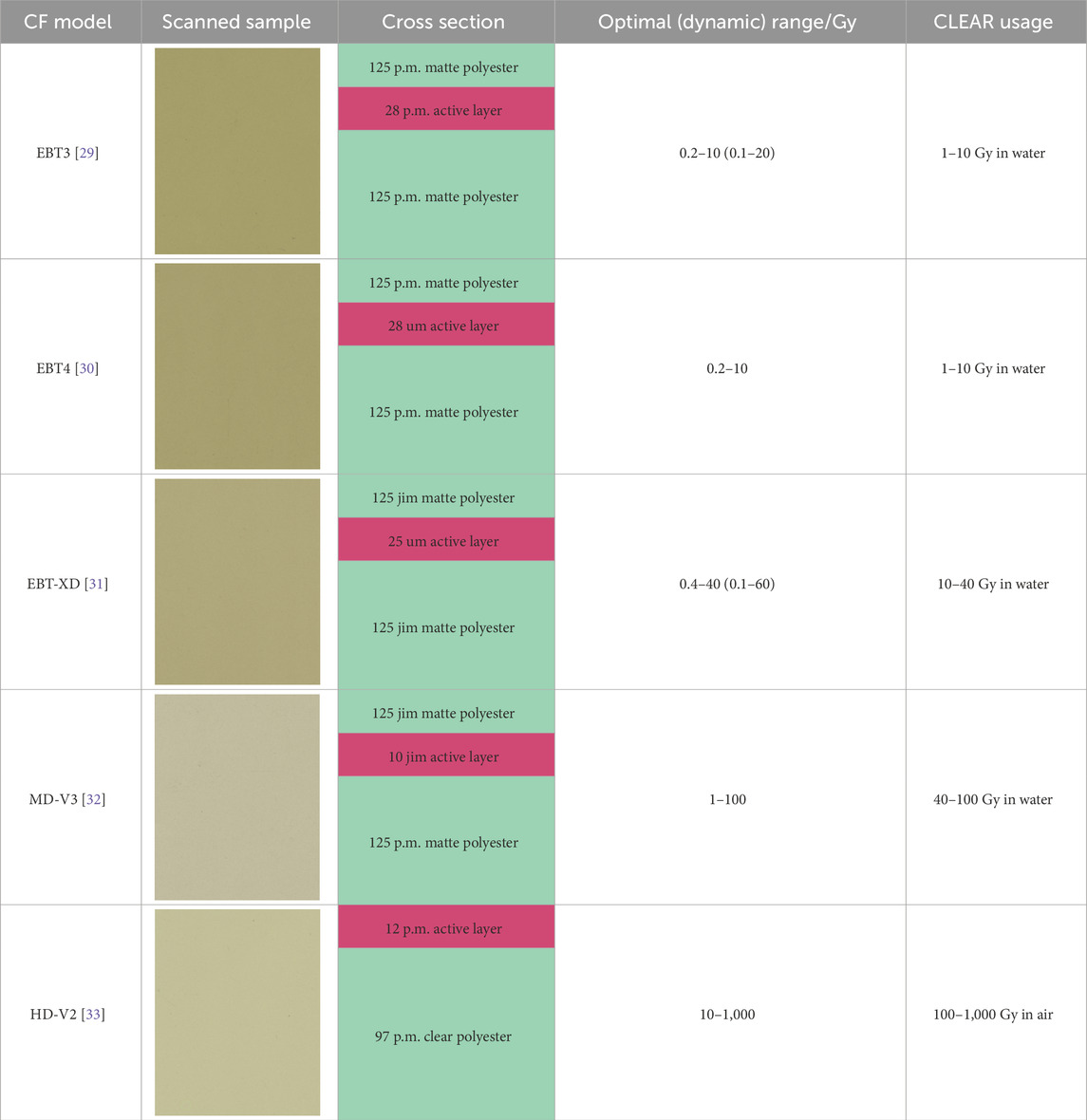
Table 1. Properties of the different models of Gafchromic™ RCFs used at CLEAR.

2.2 RCF handling and preparation

Due to the physical nature of the RCFs and the method of data retrieval, caution is necessary in their storage, preparation and handling to minimise potential uncertainties. In particular, it is essential to limit the splitting of the polyester substrates protecting the active layer, as well as light exposure, the presence of impurities such as dirt, dust and grease, and the formation of scratches, to ensure reliable dosimetry with RCFs. This section will detail good practices for RCF handling and outline strategies for mitigating such effects within the RCF protocol.

2.2.1 RCF handling

The EBT3, EBT4, EBT-XD, and MD-V3 models gain robustness by sandwiching the active layer between two polyester sheets. The design allows them to be irradiated in a water phantom for short periods and handled with bare hands. However, handling with bare hands can transfer fingerprints and impurities, which distort the dose distribution. While it is possible to wipe the RCF pieces clean with an alcohol swab or to handle them by the edges, at CLEAR we prefer to use gloves to ensure consistency when managing large numbers of RCFs.

Despite the sandwich construction, we have observed that water diffuses a few millimetres into the active layer during irradiations in liquid water phantoms. The study by Aldelaijan et. al demonstrates that water not only diffuses from the edges but also penetrates through the RCF faces to some degree. They conclude that short submersions of around 30 min yield negligible impact, whereas longer immersion periods should be corrected for [37] As for the HD-V2 model, which have the humidity sensitive active layer fully exposed, water must be completely avoided and it must in general be handled with more care.

The Gafchromic™ RCF models are relatively insensitive to indoor artificial light and can be left exposed for short periods without noticeable effects. However, they are very sensitive to UV light—even to artificial light containing UV components—which can cause darkening with prolonged exposure [38, 39]. Therefore, it is crucial that the RCFs are stored in an opaque envelope or container when not in use to avoid unnecessary uncertainties. At CLEAR we have purchased small, black antistatic bags—intended for storing electronic components—for the storage of cut RCF pieces.

Another factor to consider is the temperature stability of the RCFs. According to Ashland, EBT3 RCFs are stable up to 60 °C, but they recommend storing them below 25 °C [29]. A study by Trivedi et al. showed that storing RCFs in varying temperatures can lead to self-development, effectively shifting their sensitivity [40]. Therefore, it is good practice to store RCFs not only below 25 °C, but ideally in a temperature-controlled environment.

2.2.2 Cutting and labelling

Gafchromic™ RCFs are manufactured in sheets measuring $203\text{\hspace{0.17em}mm}\times 254\text{\hspace{0.17em}mm}$. At the CLEAR facility, a laser machine (Epilog Fusion Maker 12) has been acquired to systematically cut these sheets into $35\text{\hspace{0.17em}mm}\times 40.5\text{\hspace{0.17em}mm}$ pieces—a suitable size to capture most of the electron beam after scattering through approximately 15 cm of water, including an extra margin for water diffusion [37]. These dimensions are also tailored to fit the 3D-printed sample holders used for irradiations at CLEAR.

The laser cutting system is additionally used to engrave and uniquely label the cut RCF pieces. This ensures easy identification and maintenance of RCF orientation during irradiation, scanning, and processing. Examples of a template used for cutting and engraving the RCF sheets, as well as a prepared RCF sample, can be seen in Supplementary Figure S1.

The templates are vector graphics (SVG) files in which the cutting and engraving paths are differentiated by colour. The Epilog software includes a colour mapping feature that enables the assignment of separate laser attributes to the different colours in the SVG file, allowing for cutting and engraving to be performed in the same process. To prevent damage to the RCFs and achieve satisfactory engraving resolution, it is important to adjust the laser machine’s speed, power, and frequency carefully. Although there is currently no literature detailing the specific considerations for laser cutting RCFs, Niroomand-Rad et al. state that, if done ‘carefully’, all but a 1 mm margin around the edge can be used for dosimetry [36].

The optimal laser settings depend on the specific laser machine being used. With the Epilog Fusion Maker 12, we have observed that cutting at low speeds severely damages the RCF, even at low power. Increasing the speed generally allows for an increase in power, and the least visual damage is achieved at high speed and high power. It is important to flatten the naturally curved RCF sheets in the laser machine using adhesive tape (applied along the edges outside the engraving area) to maintain the laser’s focus during engraving.

We also explored the possibility of sealing the edges of the RCFs during the laser cutting process to prevent humidity from entering between the two substrates and diffusing into the active layer. When comparing the non-damaging laser settings, no significant difference in water resistance was observed, despite visual differences in the degree of melting at the edges. All cutting settings resulted in a persistent diffusion of 3–4 mm into the edges after 10 min of submersion in water. However, this effect was most pronounced on the three edges in contact with the sample holder. As this result also contrasts with findings presented by Aldelaijan et al., it indicates that the contact between RCFs and sample holders at CLEAR negatively affects the water diffusion and penetration behaviour [37].

As a final remark, it is important to note that Gafchromic™ RCF models contain trace amounts of chlorine, as reported by Niiroomand et al. [36]. As a safety precaution, it is crucial to cut the RCF sheets in a well-ventilated area using a laser machine connected to a fume extraction system.

2.2.3 The RCF preparation protocol at CLEAR

Based on the considerations in Sections 2.2.1 and 2.2.2, the following procedure for RCF preparation has been established at CLEAR:

1. RCFs are stored in opaque envelopes at room temperature to prevent excess darkening due to UV and ageing.

2. Gloves are used when handling the RCFs to avoid fingerprints and scratches.

3. RCF sheets are cut and engraved using a laser machine at high power and high speed, to avoid damage and ensure reproducibility and traceability.

2.3 RCF scanning

RCFs are most commonly processed using commercially available 48-bit flatbed photo scanners in transmission mode. These scanners measure the red, green, and blue (RGB) colour components of light transmitted by the RCF at a colour depth of 16 bits per channel. This process yields the fraction of incident light transmitted through the sample, $I_t/I_0$, which is mapped to a range of $2^{16}$ pixel values (PV) per colour channel, from 0 (opaque) to 65535 (transparent). Several scanning-related factors can affect the accuracy of RCF dosimetry, and this section outlines the existing effects and the mitigation techniques considered at CLEAR.

2.3.1 Timing the scans

RCFs begin to self-develop immediately upon radiation exposure, and the polymerisation process never fully ends; it continues at increasingly slower rates. Therefore, it is important to maintain consistency in the timing of RCF scanning after exposure. The post-exposure self-development of a set of EBT3 RCFs is shown in Figure 1.

Figure 1

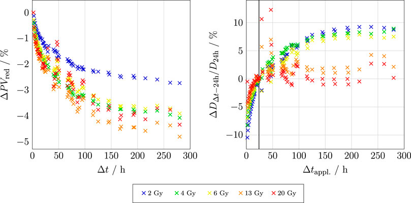
Figure 1. Left: The relative change in PV for the red channel of an EBT3 RCF as a function of time after exposure $\mathrm{\Delta }t$. Right: The dose deviation of the RCFs scanned at different times after exposure, relative to an RCF scanned at $\mathrm{\Delta }{t}_{\text{appl.}}\simeq \mathrm{\Delta }{t}_{\text{calib.}}=24\text{\hspace{0.17em}h}$, indicated by the vertical line.

The left-hand plot shows that stabilisation appears to occur more rapidly for RCFs exposed to doses at the higher end of the RCF’s dynamic range. Moreover, the steepness of these curves dictates the acceptable time window for scanning; the shorter the chosen $\mathrm{\Delta }{t}_{\text{calib.}}$ for the calibration RCFs, the smaller the acceptable absolute deviation of $\mathrm{\Delta }{t}_{\text{appl.}}$ for the application RCFs without introducing significant dose errors. The right-hand plot underscores this point by showing the induced error as a function of scanning time $\mathrm{\Delta }{t}_{\text{appl.}}$ relative to $\mathrm{\Delta }{t}_{\text{appl.}}=\mathrm{\Delta }{t}_{\text{calib.}}=24\text{\hspace{0.17em}h}$. A $\mathrm{\Delta }{t}_{\text{appl.}}$ that is sufficiently different from $\mathrm{\Delta }{t}_{\text{calib.}}$ may result in dose evaluation errors of up to 10%.

Literature therefore often suggests waiting for at least 24 h post-irradiation before scanning, as the polymerisation process is more stable at this point. Beyond 24 h and up to 14 days post exposure, the change is about 2.5% [36]. In summary, the crucial point is ensuring that the post-exposure scanning timing for the application RCFs $(\mathrm{\Delta }{t}_{\text{appl.}})$ relative to that of the calibration RCFs $(\mathrm{\Delta }{t}_{\text{calib.}})$ is minimised according to Equation 1:

$\left|1-\frac{\mathrm{\Delta }{t}_{\text{appl.}}}{\mathrm{\Delta }{t}_{\text{calib.}}}\right|\ll 1.(1)$

There is a technical possibility of mitigating this timing uncertainty by applying the ‘one-scan protocol’, which also compensates for inter-scan variabilities [41]. However, this approach relies on a recalibration by irradiating a reference RCF to a known dose that is similar to the maximum expected dose on the application RCF. This is not feasible at CLEAR because we depend on external calibration facilities.

In practice, particularly at CLEAR, where we typically scan numerous RCFs one-by-one, maintaining a consistent scanning window is challenging. Based on the aforementioned considerations, it is considered best practice to strictly adhere to $\mathrm{\Delta }t\simeq 24\text{\hspace{0.17em}h}$, as this offers a reasonable scanning time-window without risking significant error. This protocol offers a good compromise between post-exposure stabilisation and acceptable delay for most experiments at CLEAR. In research settings where the urgency of retrieving dose information is low, it may be advisable to establish a longer $\mathrm{\Delta }t$, both to further reduce the risk of timing errors and, in the case of water irradiation, to mitigate the impact of water-induced darkening [37].

2.3.2 Sample and scanner preparation

Epson photo scanners are widely used and recommended for RCF dosimetry. It is typically advised to warm up the scanner’s electronics before starting the scanning process to ensure reproducible results. If the scanner has not been used in the last hour, turning it on at least 30 min prior to scanning is sufficient. Ashland and most studies suggest performing at least 5 ‘preview’ scans in the Epson Scan software, to warm up the light source and stabilise the response, thereby limiting inter-scan variabilities [36, 39, 42]. It is important to noted that this general recommendation is more critical for cold cathode fluorescent lamp (CCFL) scanners than for LED scanners, as shown in the study by Lárraga-Gutiérrez et al. [43]. While the typically recommended scanner model (Epson Expression 11000XL) is CCFL-based, the model used at CLEAR (Epson Perfection V800 Photo) is LED based and should thus be less susceptible to warm-up effects. Nevertheless, scanner response stability is of particular importance in the CLEAR protocol because the RCFs are scanned one by one. Due to the scarcity of literature documenting the irrelevance of scanner warm-up for the V800 model, we have included five preview scans in the CLEAR protocol as a low-effort precaution.

Before starting the scanning process, it is essential to ensure that both the scanner plate and the RCFs are free from impurities. Both the scanner plate and RCF can be wiped clean with alcohol, and gloves or a vacuum suction pen should be used to position the RCFs on the scanner. At CLEAR, where the RCFs are often irradiated in a water phantom, water stains frequently appear on the RCFs, and these must be removed before scanning. As illustrated in Figure 2, such artefacts can significantly affect the pixel value and eventually the dose calculation.

Figure 2

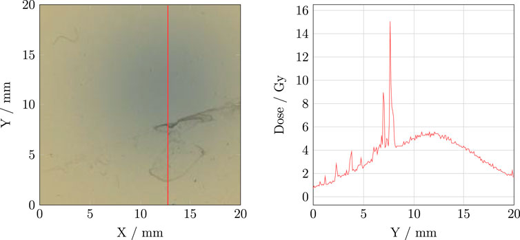
Figure 2. Left: An example of an RCF with water residues. Right: The corresponding vertical dose profile.

2.3.3 Positioning RCFs on the scanner

The positioning of RCFs on the scanner may significantly impact the results due to the orientation of the RCF polymers and lateral response artifacts (LRA)—which refer to the systematic dependency of measured PVs on the lateral position of the RCF relative to the centre of the scanner. LRA is primarily attributed to the polarisation of light transmitted through the RCF by the polymers in the active layer. The scanner light passes via a set of mirrors and a lens before reaching the image sensor, but the angle of incidence increases with the distance from the centre of the scanner [29]. As a result, RCFs scanned closer to the edges of the scanner appear darker, and the deviation also increases with decreasing PV (i.e., for darker RCFs) [36, 44]. At CLEAR, we have previously found that dose evaluation errors of up to 10% can arise from a lateral offset of the application RCF relative to the calibration RCF during scanning with the V800 model [42].

For RCFs that are large relative to the scanner, the LRA can be mitigated using techniques such as multi-channel processing—which is discussed in section 2.5—and LRA correction matrices, particularly for higher-precision measurements and/or for larger RCFs or multiple RCFs scanned simultaneously [45]. However, using a scanner that is large relative to the RCF is the easiest way to limit the LRA, and Ashland specifically recommends the 11000XL model due to its large scanning area of $310\times$437 mm².

In addition to the lamp, the smaller scanning area ($216\times$ 297 mm²) of the V800 model used at CLEAR is a significant difference compared to the 11000XL model [43]. However, this is considered acceptable due to the small dimensions of the RCF pieces used at CLEAR ($40\times$ 35 mm²) relative to the scanner surface—which are scanned one by one, centred on the scanner to limit the LRA. Consistent positioning of the RCFs on the scanner is ensured by a custom-made scanner mask with different inserts for different RCF sizes, as shown in Figure 3.

Figure 3

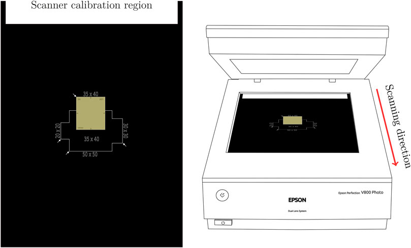
Figure 3. Left: The scanner mask used for reproducible positioning of the RCFs. Right: The Epson Perfection V800 Photo scanner with positioning of the mask in the scanner relative to the scanning direction.

It is essential that the mask itself is positioned consistently on the scanner surface and that the ‘calibration region’ closest to the starting point of the scan is left blank to ensure proper scanner response calibration.

In addition to ensuring consistent RCF positioning, the scanner mask aids in maintaining a consistent orientation of the RCFs throughout the scanning process. It is a well-known fact that RCF scans are orientation dependent due to the alignment of the polymers in the active layer [39, 46–48]. We have previously reported that increasing relative orientation differences between calibration and application RCFs can yield dose evaluation errors reaching 27% at 90° for an EBT3 RCF exposed to 5 Gy [49]. The choice scanning orientation—e.g. landscape or portrait orientation relative to the uncut sheet—is unimportant; however, it is crucial that the chosen orientation remains consistent between calibration and application RCFs. At CLEAR, we consistently scan in landscape orientation due to the design of the cutting templates.

As a remark, the natural curvature of Gafchromic™ RCF sheets may also affect the scanner response. For a full sheet on a flat surface, the maximum distance between the surface and the RCF is typically in the range of 1–2 mm, depending on the model and production lot. Therefore, particularly for large samples, it is recommended to flatten the RCF on the scanner using a clear glass plate that is 3–4 mm thick to mitigate the potential error in pixel value reading of 1.2% per millimetre offset from the light source [36, 39]. If using a flattening plate, it is important to use it consistently for both calibration and application RCFs. However, at CLEAR, we typically cut RCF sheets into small enough pieces (less than 20% of the height of the full sheet) to largely mitigate this effect, making the consistent use of a glass plate an unnecessary complication.

Lastly, it is crucial to remember that a calibration curve is only valid for a given RFDS, which includes the scanner. This may pose challenges for inter-facility collaborations because using RCFs from an external RFDS might be desired for consistency and comparability during experiments at CLEAR. However, even if the scanner of the external RFDS is the same model as the scanner at CLEAR, the results may differ significantly. An example of the potential error that can arise from using a different scanner is illustrated in Supplementary Figure S2. Moreover, since CLEAR lacks calibration capability, users cannot easily establish a new RFDS for their RCFs using the scanner at CLEAR. Additionally, unless the established $\mathrm{\Delta }t$ of the RFDS is sufficiently long and/or the corresponding scanner is in close proximity to the irradiation facility, timing the scans within a reasonable margin can be challenging. Equally, re-establishing the RFDS by re-scanning the external calibration set at CLEAR will impose a shift of the $\mathrm{\Delta }t$ which may not be compatible with experimental time constraints. The simplest way to mitigate this is for users to either fully rely on the RFDS at CLEAR, or to construct multiple calibration curves (for various $\mathrm{\Delta }t$), which allows for greater flexibility in post-experimental scanning times.

2.3.4 Scanning software settings

It is important to use appropriate settings in the scanning software when digitising RCFs. According to common practice and literature recommendations, transmission mode is used for RCF scanning, with all image corrections features turned off, and the image type set to ‘48-bit color’ [50]. Ashland provides detailed instructions for the Epson Scan software, which detail the settings used for scanning at CLEAR [39]. Scanned images are stored as TIFF files to maintain adequate bit depth and ensure lossless compression.

Regarding scanner resolution, Gafchromic™ RCF models have a spatial resolution of 25 µm or smaller, with the achievable resolution limited by the scanning system [29]. For applications involving large and uniform radiation fields, a resolution of 72 dpi (0.36 mm pixel size) is sufficient; higher resolutions can increase measurement noise [51]. However, for smaller and/or non-uniform fields, it may be necessary to increase the resolution to better capture the dose distribution [36]. This adjustment comes at the cost of increased scanning time, image size and processing time. Above all, it is crucial to maintain identical scanner settings between calibration and application RCFs. Given that the typical VHEE beam at CLEAR has a Gaussian distribution with 1σ beam sizes down to approximately $1\mathrm{m}\mathrm{m}$ in air, the RCFs are consistently scanned at a resolution of 300 dpi ($0.085\mathrm{m}\mathrm{m}$ pixel size), to ensure accurate capture of the distribution for all beams.

2.3.5 Scanning repetitions

Unless the one-scan protocol mentioned in section 2.3.1 is employed—which has the added benefit of avoiding inter-scan variabilities [41]—it is recommended to mitigate these variabilities by performing repeat scans of each RCF and using the average for evaluation [51]. However, this approach can be time-consuming for large batches of RCFs, as is typically the case at CLEAR.

Lewis and Devic proposed mitigating this by including a piece of unexposed RCF in every scan to serve as a reference for scanner response [52]. This strategy is straightforward to implement, and can be used simultaneously for background evaluation and eventual subtraction, as discussed in section 2.4. Provided that the reference is properly aligned with the application RCF in the scanning direction, there should be no LRA difference to compensate for. Additionally, studies have shown that repeated scans of an unexposed RCF do not cause any permanent darkening, indicating that using such a reference repeatedly should not induce artificial offsets [41, 52].

2.3.6 Summary: The CLEAR scanning procedure

Taking into account all the considerations concerning RCF scanning, we have developed a procedure that optimises accuracy while maintaining the necessary efficiency for use at CLEAR:

1. Ensure all calibration and application RCFs are scanned at the same time $\mathrm{\Delta }t\ge 24\text{\hspace{0.17em}h}$ post-irradiation.

2. Switch on the scanner 30 min before starting the scanning to warm up the scanner electronics.

3. Clean the scanner surface and RCFs if they are dirty.

4. Perform five preview scans to warm up the scanner lamp and stabilise the scanner response.

5. Position the RCFs at the centre of the scanner and with consistent orientation using the scanner mask.

6. Ensure the scanner settings are according to protocol, without colour corrections.

2.4 RCF calibration

Each production lot of RCFs must be calibrated to establish a relationship between level of darkening and absorbed dose. Since there are no established VHEE reference beams, external clinical low-energy electron beams are used for RCF calibration in the CLEAR protocol. Previous VHEE dosimetry studies have reported agreement between RCF dose measurements and Monte Carlo simulations, where the RCFs were calibrated to clinical 15–20 MeV electron beams [8, 27, 28]. This indicates that a low-energy RCF calibration is valid for VHEE applications.

RCFs used at CLEAR are typically calibrated using the Oriatron eRT6 linac at Lausanne University Hospital (CHUV) [53], or a Varian TrueBeam medical linac at the Geneva University Hospitals (HUG). Both calibration setups provide a 6 MeV electron beam and calibrate the RCFs to a secondary standard ionisation chamber placed behind a 1 cm slab of solid water. It is important to note that for applications where the experimental submersion time is well-defined, calibration in liquid water should be considered if feasible, as it may better represent the RCF response, including diffusion and penetration effects [37]. The ionisation chambers are calibrated to measure dose to water and are traceable to the primary standard at the Swiss Federal Institute of Metrology (METAS). There are differences in the type of ionisation chamber, the field shape and size, and the temporal beam structure between the two setups. For example, the eRT6 has a circular field while the TrueBeam features a square field. A comparison of the remaining parameters for the two facilities is presented in Table 2, and an illustration of the calibration setups is presented in Figure 4.

Table 2

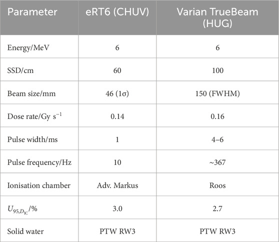
Table 2. The beam parameters used for RCF calibration at eRT6 at CHUV and the Varian TrueBeam medical linac at HUG.

Figure 4

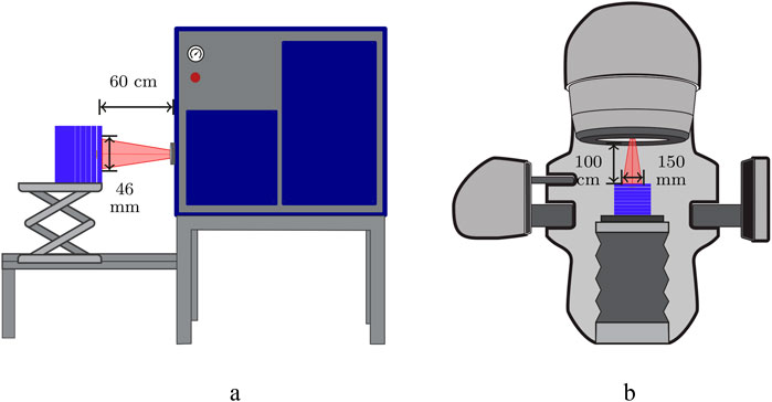
Figure 4. RCF calibration setups in solid water using low-energy electrons and ionisation chambers. (a) eRT6 linac at CHUV. (b) Varian TrueBeam at HUG.

RCF calibration involves exposing samples to a sufficient number of known doses within the dynamic range of the RCF model to establish a relationship between dose and darkening level. The required number of dose-points depends on the type of fitting function and the desired range of the calibration curve. According to Ashland, six to eight dose-points $D_{\text{calib.},n}$ arranged in geometric progression are sufficient when using a rational calibration function, such as the one in Equation 4, because this function captures the physical nature of the RCF development [29, 31]. The dose points are determined according to $D_{\text{calib.},n}=D_{\text{calib.},1}{r}^{n-1}$, where the common ratio $r$ is selected based on the dose range of interest and and the desired number of calibration points. This approach ensures a higher density of dose points in the low end of the range, where the RCF response is more non-linear. Importantly, multiple film pieces should be calibrated to the same dose in order to enable meaningful uncertainty estimations.

The RCF calibrations of the RFDS at CLEAR typically include a few additional dose points (8–12 in total) to cover the entire dynamic range of the RCF. For each dose point, two samples are calibrated simultaneously by stacking them within the solid water phantom. This approach adds statistical robustness without increasing calibration time through separate irradiations and without imposing notable gradients between the two RCFs. If feasible, a higher number of samples per dose point can be utilised to improve statistics and uncertainty estimates. Additionally, including extra dose points for accuracy evaluation of the calibration curve is good practice.

2.4.1 Establishing the calibration curves

To establish a calibration curve, a response variable that describes the dose dependency of the RCF lot must be selected. From the TIFF files of the scanned calibration RCFs, a stack of three 2D arrays corresponding to the responses of the red, green and blue channels is extracted. A curve relating dose to the chosen response variable is established separately for each colour.

There are three response variables that recur in literature: PV, optical density (OD), and net optical density (nOD). PV is often preferred for its simplicity, since the values are obtained directly from the 2D images from each colour channel $x$. The more widely used choice is OD, which is related to PV according to Equation 2:

${OD}_x=-\mathrm{l}\mathrm{n}\left(\frac{{PV}_x}{65535}\right),(2)$

where 65535 represents the RGB colour space of the scanner, as described in section 2.3. The conversion to OD is preferred because this quantity exhibits a more linear relationship behaviour with dose compared to PV and requires fewer non-linear terms to fit the inherently non-linear dose-response of RCFs [24]. This can be further extended to nOD by subtracting the mean OD of an unexposed RCF $⟨{OD}_{x,0}⟩$ from the OD of an exposed RCF ${OD}_x$ according to Equation 3:

${nOD}_x={OD}_x-⟨{OD}_{x,0}⟩.(3)$

Since there is no pixel-to-pixel correspondence between the unexposed and exposed RCFs, the mean OD across a region of interest (ROI) of the unexposed RCF is subtracted from the OD maps of the exposed RCFs to generate the corresponding nOD maps. This method accounts for the ageing of the RCF lot and is therefore recommended [50]. Ideally, the background should be obtained from the same RCF piece before irradiation. However, due to the number of samples used at CLEAR and the fact that the films are scanned individually, one RCF piece is typically kept from each sheet to serve as background for all irradiated RCFs from that sheet. In the context of irradiation in water, it may be beneficial to establish a background using an unexposed RCF that has been submerged in water in the same configuration as the irradiated RCFs to account for water diffusion effects [37].

A calibration set consists of RCF samples that have been exposed to a uniform field of known doses provided by the ionisation chamber at the calibration facility. To establish the calibration curve, an ROI must be determined that omits the edges and engravings of the RCF, is fully covered by the uniform field, and is large enough for a histogram of all PVs to result in a normal distribution with a measurable standard deviation [36]. At CLEAR, an ROI of $150\times 150$ pixels—corresponding to $12.75\times 12.75\mathrm{m}{\mathrm{m}}^{\mathrm{2}}$ at 300 dpi—centred on the RCF is selected. An example of an EBT3 calibration set is shown in Supplementary Figure S3. For each RCF in the calibration set, the mean nOD within the ROI is calculated, and the response of each dose point is the mean response between the RCF pieces exposed to the same dose.

There are numerous variants of fitting functions in literature; however it is essential to choose a function that most accurately represents the RCF’s physical dose-response and fits the calibration points. The darkening of RCFs increases with exposure but approaches a near-constant value towards the end of the dynamic range (saturation). To this end, there are generally three families of functions that express this behaviour: rational, polynomial and exponential functions. Devic et al. showed that the choice may depend on the specific RFDS [54]. More generally, the performance of each function will depend on the number of calibration dose points $D_{\text{IC}}$ and the dose-range.

Ashland recommends rational functions of the form in Equation 4, as proposed by Micke et al. [55]:

${nOD}_x\left(D\right)=-\mathrm{l}\mathrm{n}\left(\frac{a_x+b_{x}D}{c_x+D}\right),(4)$

where $a_x$, $b_x$ and $c_x$ are fitting parameters for colour channel $x$. Such functions align more closely with the inherent nature of the RCF, as opposed to polynomial functions, which do not necessarily reflect the physical properties of the RCFs outside the range of the fitted data points [33].

At CLEAR, we apply the fitting function in Equation 4, and Figure 5 shows the calibration curves for the different RCF models used. Visually, it is evident that Equation 4 fits the calibration points of the EBT3, EBT-XD, and MD-V3 models well, with the fit lying within 0.2% of the ionisation chamber measurement $D_{\text{IC}}$, which is less than the uncertainty $U_{95,D_{\text{IC}}}$. The exception is HD-V2, for which we speculate that the large uncertainty is due to environmental exposure or handling—factors to which it is more sensitive, as mentioned in Section 2.1. However, since HD-V2 are used less frequently, we do not currently have enough data to verify this.

Figure 5

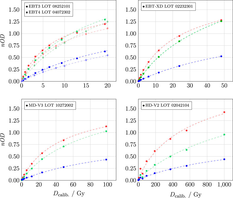
Figure 5. Calibration curves for different RCF models. The colours correspond to the respective colour channels, with circles representing the measurements, and the dashed lines indicating the fitted values.

The uncertainties in calculated doses from RCFs result from a convolution of various factors, which—together with inherent RCF imperfections, inconsistent handling, and scanner response—also include uncertainties from the calibration process, such as those associated with the calibration dose $D_{\text{IC}}$ and the fitting procedure. Estimating the uncertainty for a given calibration curve has been discussed by Devic et al., where the error in dose response, ${\sigma }_{{\mathit{nOD}}_x}$, is expressed via error propagation from ${\sigma }_{{\mathit{PV}}_x}$ via ${\sigma }_{{\mathit{OD}}_x}$ [54, 56]. These steps are also outlined in Section S5. To estimate the overall calibration uncertainty, we use orthogonal distance regression (ODR) for curve fitting, which calculates the perpendicular distance from the data points to the fitted line. This approach takes into account uncertainties in both the calibration dose $({\sigma }_{D_{\text{IC}}})$ and nOD $({\sigma }_{\mathit{nOD}})$ to construct the calibration curve [57]. The related uncertainty may be estimated by error propagation, as outlined in section Section S5.

2.4.2 Calibration validity

As stated in Section 2.4, calibrating each lot of RCFs—even if they are of the same model—is crucial to account for inter-lot variability. Supplementary Figure S4 shows an example of the calibration offset between different lots of EBT3 RCFs. Applying a calibration curve from a different lot may lead to dose estimation errors in the order of 20%.

Moreover, as discussed in Section 2.3.1, it is important to maintain consistency in the post-exposure scanning timing $\mathrm{\Delta }t$ for calibration and application RCFs to minimise errors arising from the continuous post-irradiation development of the RCFs.

There is a misconception that RCF ageing can be compensated for by re-scanning the calibration set simultaneously with scanning the application RCFs and updating the calibration curve. This practice can introduce significant errors in the calculated dose due to the considerable time discrepancy in $\mathrm{\Delta }t$ between calibration and application RCFs. Supplementary Figure S5 displays an example of an application RCF exposed to a known dose—scanned at $\mathrm{\Delta }{t}_{\text{appl.}}=24\text{\hspace{0.17em}h}$—and evaluated using calibration curves scanned at a $\mathrm{\Delta }{t}_{\text{calib.}}$ of 24 h and 233 days post-irradiation. The ‘updated’ calibration imposed more than a doubling of the dose error of the application RCF compared to the scenario where $\mathrm{\Delta }{t}_{\text{calib.}}=\mathrm{\Delta }{t}_{\text{appl.}}=24\text{\hspace{0.17em}h}$.

The rate of post-irradiation development is significantly higher than the natural self-development caused by other environmental factors, which are collectively referred to as ageing. For high accuracy, it is advised to update the calibration curve regularly by re-calibrating the lot. However, due to the lack of calibration capabilities at CLEAR, it is challenging to schedule systematic re-calibrations. Typically, a given production lot will be used at CLEAR for up to a year after calibration. To mitigate the effects of RCF ageing, it is recommended to ensure stable storage conditions, as outlined in Section 2.2.1, and to use nOD as response variable, as it effectively accounts for the drift of the unexposed RCFs [50].

2.4.3 Summary: The CLEAR calibration procedure

Based on the considerations discussed in Section 2.4, the following procedure for RCF calibration has been established at CLEAR:

1. Net optical density $nOD$ is used as the response variable to account for ageing.

2. RCFs are calibrated against a secondary standard ionisation chamber using a low-energy electron linac that provides a sufficiently large and uniform field at a conventional dose-rate.

3. 8 to 12 dose points arranged in geometric progression are used to calibrate the full dynamic range of a given RCF model. This includes two to three dose points for calibration verification.

4. The calibration RCFs are scanned at a time $\mathrm{\Delta }t\simeq 24\mathrm{h}$ post irradiation.

5. The calibration points ${nOD}_x(D_{\text{IC}})$ for each colour channel $x$ are fitted to the rational function in Equation 4, which reflects the physical nature of RCFs.

2.5 RCF processing and analysis

To retrieve dose distributions from application RCFs, calibration curves are applied to the digitised images. RCF processing can be performed using dedicated, commercial programs, such as FilmQAPro (Ashland) and radiochromic.com, which are accessible to some facilities, particularly clinics. Alternatively, open-source image processing software such as ImageJ—which has its own macro language for customisation and task automation—is commonly used among researchers. At CLEAR, a toolkit based on the scientific Python stack has been developed in-house for RCF processing and is under continuous improvement [58].

A key difference in RCF processing arises from whether the dose is calculated using information from one or multiple of the three (RGB) calibration curves. This section details and compares these two approaches—single-channel and multi-channel processing—which have both been utilised at CLEAR.

2.5.1 Single-channel RCF dosimetry

For accurate dosimetry using a single colour channel, it is essential to select the channel that exhibits the highest sensitivity, defined according to Equation 5:

$S=\frac{\partial {nOD}_x}{\partial D}.(5)$

Literature reviews indicate that the red channel is the most commonly used channel for single channel dosimetry, based on the fact that Gafchromic™ RCFs have maximum absorption in the red band (at approximately 633 nm). However, as shown in Figure 5 in Section 2.4, the red channel is not necessarily the most sensitive channel for all dose ranges and RCF models. The sensitivities of the calibration curves are displayed in Figure 6 and illustrate, for example, that beyond 3–4 Gy, the green channel is more sensitive than the red for EBT3. It is also evident why the blue channel is hardly used for single-channel dosimetry; nevertheless, it should be noted that it has been shown to be useful for extending the dynamic range of the RCFs [59].

Figure 6

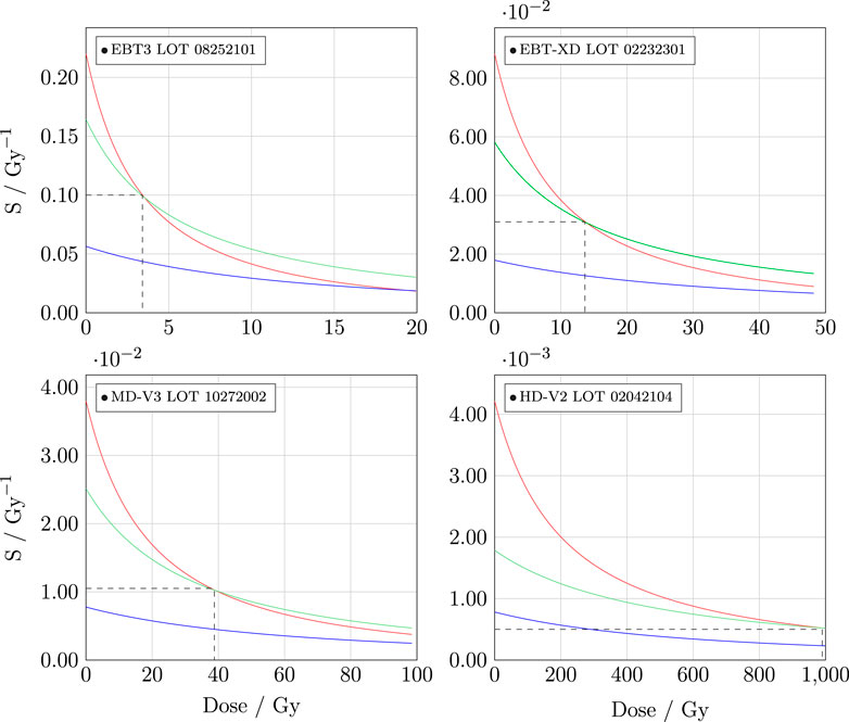
Figure 6. Sensitvity of the different calibration functions in Figure 5.

Using a single colour channel $x$, the dose is calculated directly from the inverse of the calibration function in Equation 4 according to Equation 6:

$D=\frac{a_x-c_x{\mathrm{e}}^{-{nOD}_x}}{{\mathrm{e}}^{-{nOD}_x}-b_x}.(6)$

The corresponding uncertainty, ${\sigma }_D$, is calculated by error propagation, outlined in Supplementary Equation S5.

The single-channel processing method has been employed at CLEAR since 2019. However, when determining the dose on the RCF using a single colour channel, the entire response is converted to dose. Due to the numerous potential uncertainties arising from RCF handling and scanning, this approach may lead to potentially significant errors in dose estimation, particularly as certain artefacts yield larger responses in specific channels. This motivated the transition to multi-channel dosimetry, which weighs the responses from the three channels channels to minimise the influence of non-dose-dependent artefacts.

2.5.2 Multi-channel RCF dosimetry

Dedicated commercial tools such as FilmQAPro and radiochromic.com offer multi-channel processing capabilities, utilising information from all three colour channels for dose evaluation. Multi-channel processing separates the RCF response into a dose-dependent component and a dose-independent perturbation [36]. By estimating the perturbation that minimises the difference between doses calculated from each individual colour channel, the noise from the dose-distribution is reduced.

The multi-channel method can mitigate issues such as variations in thickness across the active layer and scanner artefacts—including LRA, noise, and, to some extent, impurities—by optimising the dose value to the most probable value using information from all three calibration curves. The multi-channel method was first proposed by Micke et al. [55], followed by Mayer et al., who proposed an implementable solution to the optimisation problem [60]. This solution expresses the dose as a Taylor expansion with a perturbation, and minimises the cost function, which represents the difference between the true (common) dose $D$ and the channel-dependent responses, encompassing both the dose and the perturbation.

As of 2025, multi-channel processing has been integrated into the RCF processing software at CLEAR [58]. The dose on the RCF is evaluated according to Equation 7, which was introduced by Mayer et al.:

$D=\frac{⟨D⟩-RS\cdot \frac{{\sum }_x{D}_x\cdot D_x^{\prime }}{{\sum }_x{D}_x^{\prime }}}{1-RS}.(7)$

Here, $⟨D⟩$ is the average dose estimated using all colour channels, according to Equation 8:

$⟨D⟩=\frac{1}{3}{\displaystyle \sum _x}{D}_x,(8)$

and $D_x^{\prime }$ is the derivative of the dose function w.r.t. the response variable ${nOD}_x$, expressed according to Equation 9:

$D_x^{\prime }=\frac{\partial D\left({nOD}_x\right)}{\partial {nOD}_x}={\mathrm{e}}^{{\mathit{nOD}}_x}\cdot \frac{a_x-b_x{c}_x}{{\left(b_x{\mathrm{e}}^{{\mathit{nOD}}_x}-1\right)}^2},(9)$

while $RS$ is the relative slope of the colour channels, given by Equation 10:

$RS=\frac{1}{3}\frac{{\left({\sum }_x{D}_x^{\prime }\right)}^2}{{\sum }_x{D^{\prime }}_x^2}.(10)$

The corresponding uncertainty is calculated by further propagating the single channel dose uncertainty ${\sigma }_D$ as outlined in Equation S5. The accuracy of this method within the context of the CLEAR protocol is currently under evaluation. Examples of relative errors using red, green and multi-channel can be seen in Supplementary Figure S6.

2.5.3 Summary: The CLEAR RCF processing procedure

Based on the considerations described in Section 2.5, the following procedure is followed for RCF processing at CLEAR:

1. Application RCFs are scanned at $\mathrm{\Delta }{t}_{\text{appl.}}\simeq \mathrm{\Delta }{t}_{\text{calib.}}\simeq 24\mathrm{h}$.

2. Between 2019–2024 the single-channel method was the sole approach used to convert RCF response to dose, selecting the colour channel with the highest sensitivity for the relevant the dose-regime.

3. Since 2025, the multi-channel method has been implemented to achieve noise reduction and higher accuracy. Its performance is currently being evaluated, and it is used alongside the single-processing method.

3 Protocol validation with passive dosimeters

To evaluate both the accuracy of our RCF dosimetry for typical CLEAR experiments and the robustness of the described RCF dosimetry protocol, we conducted a series of experiments comparing our RCF dosimetry with three other passive dosimeters: alanine dosimeters (ADs), radiophotoluminescence dosimeters (RPLDs), and dosimetry phantoms (DPs). These comparative measurements were performed using a geometry similar to that of a typical irradiation at CLEAR, where the ADs, RPLDs, and DPs were positioned relative to the RCFs in the same manner as typical samples.

3.1 Irradiation setup at CLEAR

CLEAR features a Cartesian robot capable of positioning custom 3D-printed sample holders into and out of the beam without manual intervention [61]. This robot offers significant advantages in many irradiation experiments by ensuring both reproducible sample positioning and the ability to irradiate multiple samples in a relatively short time. This capability is particularly crucial, as a 30-min cool-down period is required to access CLEAR after the beam has been switched off, complicating manual interventions between irradiations¹.

An illustration of the irradiation setup, including the robot, is shown in Figure 7. The robot employs a sample grabber to pick up sample holders from a storage area outside of the beam and place them in front of the beam. The sample storage area has a capacity of up to 32 sample holders and features optional temperature control. Additionally, a water phantom mounted on a vertical stage is positioned within the robot’s boundaries along the beam path, enabling sample irradiations in water.

Figure 7

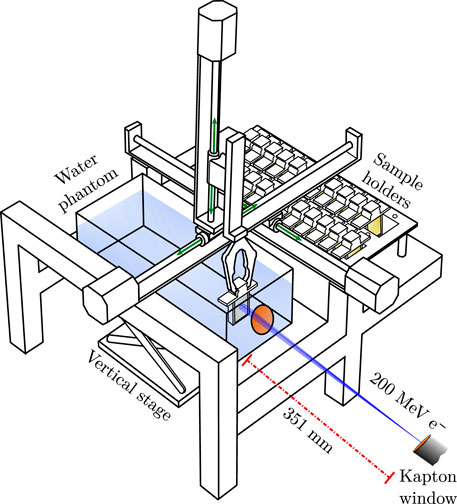
Figure 7. A drawing of the robot holding a sample holder inside the water phantom, with the path of the beam indicated in blue. The illustration is adapted from [22].

Typical irradiation experiments at CLEAR are conducted inside the water phantom using a Gaussian beam. The chosen irradiation depth varies and depends on the sample geometry and dose requirements of each experiment. Effectively, this represents an optimisation between increasing the beam size and improving uniformity across the sample, while also reaching the required dose—particularly at UHDR, which is a single-pulse modality. It is important to note that varying the irradiation depth alters the particle spectra, also known as beam quality, which introduces additional challenges regarding the comparability of experiments.

Figure 8 illustrates the typical evolution of peak dose and beam size throughout the water phantom for a Gaussian beam at CLEAR [62]. The initial phase space of the beam—defined by its Twiss parameters—affects the steepness of the curves, indicating that the irradiation depth for a given beam size depends on the initial beam conditions. The overall evolution aligns with expectations for a Gaussian VHEE beam, contrasting with the flatter build-up for uniform beams as demonstrated by Böhlen et al. [8]. Similar simulations have been experimentally confirmed to be representative of the beam at CLEAR [63].

Figure 8

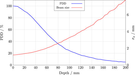
Figure 8. A typical percentage-depth-dose (PDD) curve and beam size evolution for the CLEAR beam in water. These curves were obtained from Monte Carlo simulations using TOPAS, as outlined in Section S6.

For the comparative measurements between the RCFs and the RPLDs and DPs, different mean dose rates were employed to study the relative agreement at both CDR and UHDR. The CDR irradiation conditions at the CLEAR facility utilise one bunch per pulse, with a bunch charge on the order of 100 pC and a bunch length of approximately 1–5 ps, delivered at a pulse repetition rate of 0.833 Hz. In contrast, UHDR irradiation conditions deliver a single pulse consisting of a train of bunches spaced at a frequency of 1.5 GHz. The charge per pulse (and thus dose per pulse) is determined by the number of bunches within the train and hence the pulse width, which can be up to $\sim$50 ns.

3.2 Comparison with alanine dosimeters

As part of our efforts to validate the RCF protocol, we collaborated with Physikalisch-Technische Bundesanstalt (PTB) in Germany to compare the agreement between RCF dosimetry at CLEAR and alanine dosimeter (AD) measurements from PTB. Additionally, the goal was to determine if the agreement varied across different energies. The RCFs and ADs were irradiated simultaneously at CLEAR and analysed at CLEAR and PTB, respectively.

Twenty samples—each consisting of a stack of four ADs, shrink-wrapped in polythene foil—were provided by PTB. Each sample was positioned on the downstream side of an EBT-XD RCF and mounted in a robot holder. The setup and dimensions of the samples and ADs are illustrated in Figure 9.

Figure 9

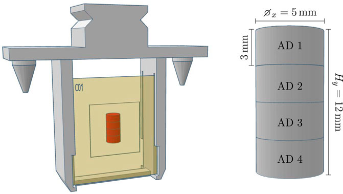
Figure 9. Left: The robot holder with a stack of four alanine pellets (indicated in red) packed in plastic and attached on the back of an RCF. Right: The stack of ADs with dimensions.

To investigate the energy dependence, four different beam energies of 50, 100, 150, and 200 MeV were targeted. Five samples were irradiated for each energy, with three targeted at 15 Gy and the remaining two were targeted at 10 and 20 Gy to cover the dose range relevant to the majority of experiments at CLEAR. The beam was delivered at CDR. For each energy, the beam size was optimised to approximately ${\sigma }_{x,y}=5.5\text{\hspace{0.17em}mm}$, minimising dose gradients across the stacks while keeping it consistent for all energies. This required adjustments to the irradiation depth at the different energies.

Both the single green channel—as the overall most sensitive channel for EBT-XD in the range of 10–20 Gy—and multi-channel processing methods were employed to evaluate the dose response of the RCFs. The mean RCF doses and standard deviations were obtained from the ROI corresponding to the positions of the two central ADs (AD two and AD 3), optimising for symmetry and uniformity. The absorbed doses to the ADs were subsequently determined at PTB by measuring the concentration of free radicals produced by ionising radiation using electron spin resonance (ESR) spectroscopy [64–66].

The dose responses of the RCFs and ADs are compared in Figure 10.

Figure 10

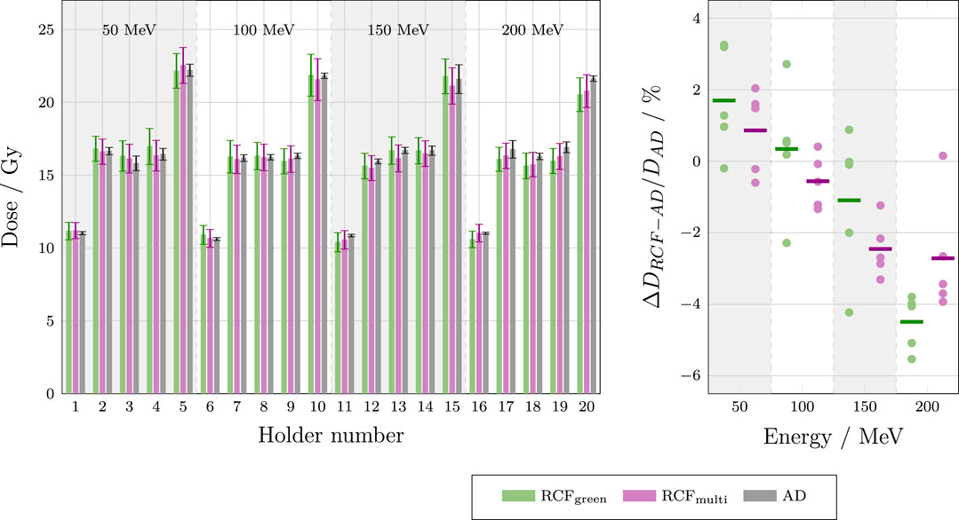
Figure 10. Left: Bar chart showing dose measurements from each sample holder of the ADs and EBT-XD RCFs, analysed using both the single green channel and the multi-channel method. The AD doses represent the averages of the two central pellets in each stack (AD two and AD 3) and are compared for 50, 100, 150 and 200 MeV. Right: Deviations between RCF and AD measurements for each beam energy.

The left-hand plot in Figure 10 shows that the dose values obtained from both the single green channel and multi-channel processing of the RCFs agree with the AD values within a single standard deviation for each sample. The right-hand plot demonstrates that both the single green channel and multi-channel RCF processing methods yield average absolute percentage deviations of less than 5% for all beam energies when compared to the AD measurements. Overall, the multi-channel method appears to perform better relative to the AD values. The observed dose overestimation of RCFs compared to ADs at lower energies, and underestimation at higher energies, is not fully understood, and additional statistics under improved irradiation conditions would be necessary to evaluate its significance.

The mean standard deviation of the RCF measurements (5.8%) is larger than of the AD measurements (1.7%) for several reasons. The dominant factor is that the small Gaussian beam (${\sigma }_{x,y}$ = 5.5 mm) is inhomogeneous across the area occupied by the ADs (5 mm$\times$3 mm), whereas the AD calibration refers to a homogeneous reference field of $10\times$10 cm². Small differences in lateral positioning of the ADs relative to the beam axis in small fields can lead to large deviations in the dose that are challenging to assess. Moreover, the effect of the inhomogeneous distribution of the free radicals on the ESR signal is not easily quantifiable.

Another source of uncertainty arises from deviations from reference conditions. The ADs were positioned in a small Gaussian field at considerable depths in water (62 mm–180 mm), while the AD calibration is based on ⁶⁰$\mathrm{C}\mathrm{o}$ irradiations under reference conditions—a homogeneous field of $10\times$10 cm² at a depth of 50 mm in water. This calibration accounts for a radiation quality factor (1.012) that corrects for the AD response to electron radiation under reference conditions—a homogeneous field of $10\times$10 cm² at reference depths of 10 mm–60 mm. For small electron fields, such as those at CLEAR, a reference depth is not even defined.

Lastly, the validity of the AD calibration is only verified for electron energies ranging from 6 to 20 MeV [67]. Although no significant energy dependence has been observed in the range 15 MeV–50 MeV when compared with RCF and ionisation chamber measurements [68], the energy range of 50 MeV–200 MeV used for irradiation at CLEAR could also introduce a source of uncertainty.

3.3 Comparison with radiophotoluminescence dosimeters

The RCF dosimetry at CLEAR has also been compared to measurements from radiophotoluminescence dosimeters (RPLDs) in collaboration with the CERN radiation working group (RADWG). An additional aim of this study was to investigate the relative agreement between the responses of the dosimeters to irradiation under both CDR and UHDR conditions. To this end, the RCFs and RPLDs were irradiated simultaneously at CLEAR and analysed at CLEAR and by the RADWG, respectively.

RPLDs are passive dosimeters made from silver-doped phosphate glass. Under radiation exposure, electron-hole pairs generated within the glass are trapped, leading to the formation of two types of optical centres: luminescence centres (RPL centres), and colour centres. When exposed to UV light, the RPL centres emit luminescence light that can be measured to estimate the absorbed dose in the glass dosimeter [69]. While this dosimetry technology is currently less commonly used in medical applications, it is widely used in environmental monitoring. At CERN, their sensitive range extends beyond traditional applications, reaching the MGy-range [70]. RPLDs offer advantages of being robust, exhibiting minimal fading effects, and allowing for repeated readouts without signal loss.

In a previous study, we compared the agreement between RPLDs and HD-V2 RCFs in air within the dose range of 30–300 Gy, finding an agreement within 10% [49]. However, the question remained whether a better agreement could be achieved in water for clinical doses and whether there was a clear dose-rate dependency.

A total of 16 RPLDs were provided by the RADWG and were irradiated alongside both EBT-XD and MD-V3 RCFs under CDR and UHDR conditions. Doses of 10, 15 and 20 Gy were targeted, which are typical for medical application experiments at CLEAR. Whereas the ADs were fixed directly downstream of an RCF, the cylindrical RPLDs were positioned between two RCFs due to their larger longitudinal $(z)$ size, as shown in Figure 11.

Figure 11

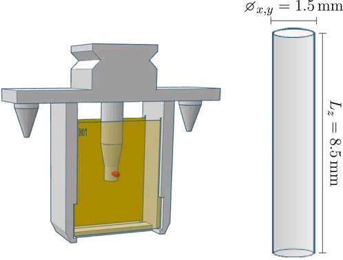
Figure 11. Left: The robot holder with an RPLD (indicated in red) positioned between two RCFs. Right: The RPLD with its dimensions.

Both the single green channel and the multi-channel processing methods were utilised to evaluate the dose response of the RCFs. The mean doses and standard deviations were obtained from an ROI corresponding to the cross-sections of the RPLDs. These results and are presented in Figure 12 along with the RPLD measurements.

Figure 12

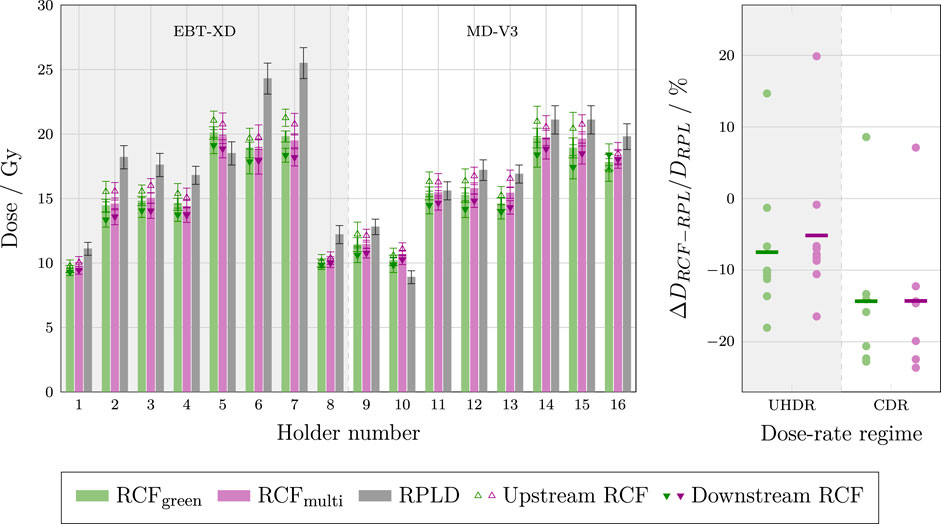
Figure 12. Left: Bar chart of the individual dose measurements of the RPLDs and various RCF types analysed using both the single green channel and the multi-channel method. The chart display the average between upstream and downstream RCFs, as well as the upstream and downstream RCF measurements. The irradiations were performed at UHDR (holders 1–7) and CDR dose-rates (holders 8–16). Right: The deviations between RCF and RPLD measurements for each dose-rate regime.

The left-hand plot shows that the dose values obtained from both the single green channel and multi-channel processing of the RCFs are generally lower and fall outside the standard deviations of the RPLD measurements. Overall, the mean standard deviation for the RCF measurements is lower than for the RPLDs, with values of 2.9% and 3.3% for the multi-channel and green-channel, respectively, compared to 4.9% for the RPLDs. The left-hand plot also shows that the relative difference between RPLD and RCF measurements is more variable than the differences observed for the ADs versus RCFs.

The right-hand plot shows that the single green channel and multi-channel processing methods yield average absolute percentage deviations of more than 5% at UHDR and more than 10% at CDR, with spreads of up to 30% relative to the RPLD measurements.

The significant and variable discrepancies observed between the RCFs and RPLDs can be attributed to multiple factors. While the wide spread in relative measurements complicates the ability to draw definitive conclusions, several known issues need to be addressed in future experiments. First, the RPLDs were firmly inserted into a hole in a resin-printed sample holder, raising the possibility that some resin may have rubbed off onto the RPLDs. Although an ultrasonic bath cleaning procedure of the RPLDs was performed before readout—resulting in a somewhat improved agreement with the RCF measurements—it is still possible that residues remain, potentially affecting the measurements.

Secondly, although RPLDs are thought to exhibit minimal dose rate effects, recent studies have indicated that exposure to dose rates differing from the calibration conditions can impact the formation of both RPL and colour centres within the dosimeter [71].

Lastly, and most importantly, the calculation of the relative dose between the RCFs and RPLDs is susceptible to misalignment errors. A slight offset between the region of the Gaussian beam intercepted by the RPLD and the ROI analysed on the RCF can contribute to the relative dose uncertainty. Given that the cross-sectional area of the RPLDs is smaller than that of the ADs, alignment inaccuracies can have a more pronounced impact on the dose recorded by the RPLDs.

3.4 Comparison with dosimetry phantoms

Finally, we compared our RCF dosimetry with measurements from ‘dosimetry phantoms’ (DPs) in collaboration with Institiut de Radiophysique (IRA) at CHUV in Switzerland. Similar to the RPLDs, we simultaneously investigated the relative responses under UHDR and CDR conditions. Upon irradiation at CLEAR, the RCFs were analysed using the described protocol, while the DPs were analysed by IRA.

The DPs are 3D-printed from $\text{ONYX}$®—a composite material of micro carbon fibre filled nylon with a density of 1.2 g cm⁻³ [72]—and each contains three LiF-100 thermoluminescent dosimeters (TLD) interleaved with approcimately 10 small $(⌀=3\text{\hspace{0.17em}mm})$EBT3 RCFs. The remaining volume of the DP is filled with rubber to prevent large air gaps. This configuration is inspired by the multi-centre UHDR dosimetry cross validation conducted at CHUV and Stanford University, which utilised a cuboid DP filled with TLDs, ADs and RCFs to compare the measurements of 8 MeV UHDR electron beams [73].

A total of 10 DPs were provided by IRA. For irradiation, each DP was positioned in a custom sample holder, between two RCFs, as illustrated in Figure 13.

Figure 13

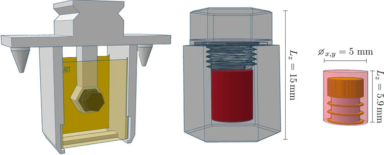
Figure 13. Left: The robot holder with the DP positioned between two RCFs. Right: The structure of the DP, highlighting its sensitive volume (in red) and dimensions.

The setup is similar to that used in radiobiology experiments at CLEAR, where there is particular interest in validating the dosimetry. In these experiments, an Eppendorf tube is typically positioned between two RCFs to evaluate the dose delivered to the samples in the tube. However, because the DPs are relatively large compared to these tubes, the separation between the two RCFs was increased from 12 mm to 20 mm to accommodate their length. We targeted 10 Gy for all holders, which is a typical dose for biological irradiations at CLEAR. The agreement among different RCF models were simultaneously investigated by interchanging between EBT3, EBT-XD and MD-V3 in the different sample holders.

For each DP, the dose and uncertainty were calculated as the mean and standard deviation across the constituent dosimeters. Both the single green channel and the multi-channel processing methods were employed to evaluate the dose response of the upstream and downstream RCFs. The RCF doses and standard deviations were obtained from an ROI corresponding to the cross-sections of the sensitive volumes of the DPs. These results are presented in Figure 14.

Figure 14

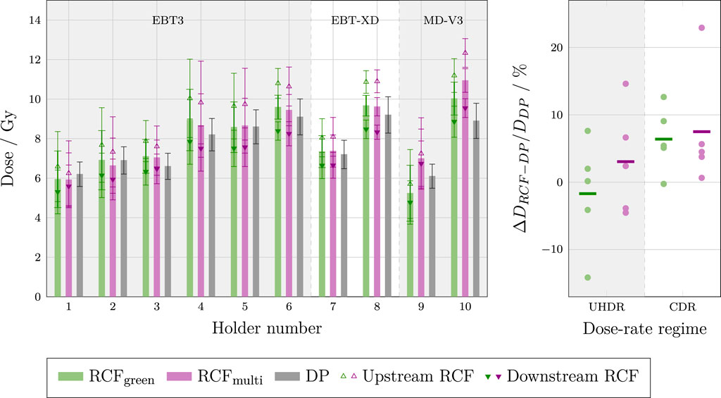
Figure 14. Left: Bar chart of dose measurements from each sample holder, displaying the dose from the DPs and the RCFs analysed using both the single green channel and the multi-channel methods. The RCF doses represent the averages between upstream and downstream films, as well as the individual upstream and downstream measurements. Holders 1–3, seven and nine were irradiated at UHDR, while holders 4–6, 8 and 10 were irradiated at CDR. Right: The deviations between RCF and DP measurements for each dose-rate regime.

The left-hand plot shows that, for most of the holders, the dose obtained from the DP is within the uncertainty range of the mean RCF response. The magnitude of the individual standard deviations can be attributed to the small beam size relative to the cross-section of the DPs, resulting in a significant transverse variation in dose. Furthermore, notable differences in doses measured by the upstream and downstream RCFs can be attributed to significant beam scattering between the two RCFs. This scattering may also contribute to the discrepancies observed between the doses determined by the RCFs and the DPs. Additionally, it is evident that the relative difference between the upstream and downstream RCFs is variable, which could indicate inconsistent beam divergence between irradiations, complicating the evaluation of measurement accuracy.

The right-hand plot shows the relative deviation between RCFs and DPs irradiated at UHDR and CDR. There seems is a larger spread in measurements at UHDR versus CDR. This discrepancy may be attributed to pulse-to-pulse position jitter, which is often more pronounced $(\simeq 1\text{\hspace{0.17em}mm})$ for UHDR irradiations than for CDR (where several pulses are accumulated). This alignment error between the sample and the centre of the beam increases the dose gradients across the DPs, significantly raising the uncertainty. In addition to the factors discussed above, several known uncertainties may help explain the discrepancies in the results. One issue is that, due to a problem with the accelerator, half of the DPs were irradiated 13 days after the other half. At IRA, the protocol involves irradiating reference TLDs in a⁶⁰$\mathrm{C}\mathrm{o}$ beam to a known reference dose on the same day as the irradiation of the TLDs being tested. This practice allows for correction of the daily sensitivity of the dosimetric system, thereby avoiding the need for additional fading corrections [34]. Since the TLD reference irradiation was performed simultaneously with half of the DP irradiations, this may imply that the measurement uncertainties for the other half are higher.

4 Conclusion

In this paper we presented a comprehensive overview and discussion of the various factors that impact the accuracy of RCF dosimetry. This evaluation was used to motivate the RCF dosimetry protocol that has been adapted for CLEAR—a research facility that relies heavily on RCFs for VHEE and UHDR studies.

With the aim of serving as a guide for similar facilities needing to adapt RCF protocols for high throughput and small or non-uniform beams, we highlighted the key principles, pitfalls and lessons learned at CLEAR. This enables informed decisions to achieve adequate accuracy while optimising time and resources for compatibility with a research setting. Strict adherence to a protocol is imperative for reliable RCF dosimetry; particularly in maintaining complete consistency in the handling of calibration and application RCFs. The scanning time $\mathrm{\Delta }t$ often presents challenges in a research setting, especially during inter-facility collaborations. We demonstrated that inconsistent post-irradiation scanning timing between calibration and application RCFs can lead to dose errors exceeding 5%.

We have identified areas for improvement in the current RCF protocol that are feasible to implement at CLEAR. Most importantly, consistently scanning the background (unirradiated) RCF simultaneously with each application RCF is a straightforward approach to mitigating inter-scan variability, as well as offsetting the ageing of the RCF lot. For RCF irradiations in water, using a background that has been submerged in the same manner and for the same duration as the application RCFs will also help offset water penetration effects.

We have verified the RCF protocol at CLEAR by comparing RCF measurements with alanine dosimeters (ADs), radiophotoluminescence dosimeters (RPLDs), and dosimetry phantoms (DPs). We achieved relative agreement between RCFs and ADs within 5% using a Gaussian beam, whilst the agreement was lower between RCFs and RPLDs and DPs. We explained that the latter inconsistencies were likely due to experimental uncertainties, such as alignment inaccuracies, which pose challenges for irradiations with small and non-uniform beams. By leveraging the experience gained from these outcomes, along with recent advancements in irradiation procedures at CLEAR, we foresee future optimised experiments yielding better agreement.

First and foremost, the development of VHEE dual scattering systems capable of generating larger and more uniform beams would significantly enhance the assessment of the RCF dosimetry accuracy relative to other dosimeters [74]. For Gaussian beams, minimising the distance between the RCF and sample, along with improving alignment and ROI selection procedures for the RCFs, would help reducing uncertainties. Lastly, particularly for UHDR irradiations, improved control of pulse-to-pulse beam position is likely to improve the results.

Data availability statement

The raw data supporting the conclusions of this article will be made available by the authors, without undue reservation. The software developed for RCF processing and analysis is available from the BeamDosimetry repository https://gitlab.cern.ch/CLEAR/dosimetry/.

Author contributions

VR: Conceptualization, Data curation, Formal Analysis, Investigation, Methodology, Software, Visualization, Writing - original draft, Writing - review and editing. JB: Conceptualization, Data curation, Formal Analysis, Investigation, Methodology, Software, Visualization, Writing - original draft, Writing - review and editing. LW: Methodology, Writing - review and editing, Investigation. MC: Investigation, Methodology, Resources, Writing - review and editing. VG: Methodology, Writing - review and editing, Resources. YA: Investigation, Writing - review and editing, Formal Analysis, Methodology, Resources, AS: Investigation, Methodology, Writing - review and editing, Formal Analysis, Resources. CB: Formal Analysis, Investigation, Methodology, Resources, Writing - review and editing. WF: Investigation, Methodology, Resources, Writing - review and editing. AG: Formal Analysis, Investigation, Writing - review and editing, Data curation, Writing - original draft. CR: Investigation, Writing - review and editing, Software. PK: Writing - review and editing, Investigation, Methodology. AM: Writing - review and editing, Investigation. SS: Supervision, Writing - review and editing, Funding acquisition. M-CV: Conceptualization, Resources, Supervision, Writing - review and editing, Methodology. MD: Conceptualization, Funding acquisition, Resources, Supervision, Writing - review and editing. RC: Conceptualization, Funding acquisition, Methodology, Project administration, Resources, Supervision, Writing - review and editing.

Funding

The author(s) declare that financial support was received for the research and/or publication of this article. This work was partly supported by the Research Council of Norway (NFR grant no. 310713) and the Science and Technology Facilities Council (STFC grant no. 2432490).

Acknowledgments

This work has to a great extent been based on the comprehensive compilation of best-practices for RCF dosimetry by Niroomand-Rad et al. in the Report of AAPM Task Group 235 [36], the numerous papers of S. Devic et al. which thoroughly describe various aspects of RCF dosimetry [24, 54, 56, 59, 75], and the literature on multichannel dosimetry by Micke et al. [55] and Mayer et al. [60]. Moreover, we have to extend our gratitude towards CHUV, HUG, PTB, and the CERN radiation working group (RADWG), for their support and useful input in calibrations and dosimetry cross-correlation experiments, which has been instrumental in this work.

Conflict of interest

The authors declare that the research was conducted in the absence of any commercial or financial relationships that could be construed as a potential conflict of interest.

Generative AI statement

The author(s) declare that no Generative AI was used in the creation of this manuscript.

Any alternative text (alt text) provided alongside figures in this article has been generated by Frontiers with the support of artificial intelligence and reasonable efforts have been made to ensure accuracy, including review by the authors wherever possible. If you identify any issues, please contact us.

Publisher’s note

All claims expressed in this article are solely those of the authors and do not necessarily represent those of their affiliated organizations, or those of the publisher, the editors and the reviewers. Any product that may be evaluated in this article, or claim that may be made by its manufacturer, is not guaranteed or endorsed by the publisher.

Supplementary material

The Supplementary Material for this article can be found online at: https://www.frontiersin.org/articles/10.3389/fphy.2025.1597079/full#supplementary-material

Footnotes

¹This is a radioprotection requirement at CLEAR, linked to its capability for material activation.

References

1. Vozenin MC, Bourhis J, Durante M. Towards clinical translation of FLASH radiotherapy. Nat Rev Clin Oncol (2022) 19(12):791–803. doi:10.1038/s41571-022-00697-z

PubMed Abstract | CrossRef Full Text | Google Scholar

2. Gao F, Yang Y, Zhu H, Wang J, Xiao D, Zhou Z, et al. First demonstration of the FLASH effect with ultrahigh dose rate high-energy X-rays. Radiother Oncol (2022) 166:44–50. doi:10.1016/J.RADONC.2021.11.004

PubMed Abstract | CrossRef Full Text | Google Scholar

3. Miles D, Sforza D, Wong JW, Gabrielson K, Aziz K, Mahesh M, et al. FLASH effects induced by orthovoltage X-rays. Int J Radiat Oncology*Biology*Physics (2023) 117:1018–27. doi:10.1016/j.ijrobp.2023.06.006

PubMed Abstract | CrossRef Full Text | Google Scholar

4. Diffenderfer ES, Verginadis II, Kim MM, Shoniyozov K, Velalopoulou A, Goia D, et al. Design, implementation, and in vivo validation of a novel proton FLASH radiation therapy system. Int J Radiat Oncol Biol Phys (2020) 106:440–8. doi:10.1016/J.IJROBP.2019.10.049

PubMed Abstract | CrossRef Full Text | Google Scholar

5. Favaudon V, Caplier L, Monceau V, Pouzoulet F, Sayarath M, Fouillade C, et al. Ultrahigh dose-rate FLASH irradiation increases the differential response between normal and tumor tissue in mice. Sci Translational Med (2014) 6:245ra93. doi:10.1126/scitranslmed.3008973

PubMed Abstract | CrossRef Full Text | Google Scholar

6. Vozenin MC, De Fornel P, Petersson K, Favaudon V, Jaccard M, Germond JF, et al. The advantage of FLASH radiotherapy confirmed in Mini-pig and Cat-cancer Patients. Clin Cancer Res : official J Am Assoc Cancer Res (2019) 25:35–42. doi:10.1158/1078-0432.CCR-17-3375

PubMed Abstract | CrossRef Full Text | Google Scholar

7. DesRosiers C, Moskvin V, Bielajew AF, Papiez L. 150-250 MeV electron beams in radiation therapy. Phys Med and Biol (2000) 45:1781–805. doi:10.1088/0031-9155/45/7/306

PubMed Abstract | CrossRef Full Text | Google Scholar

8. Böhlen TT, Germond JF, Traneus E, Bourhis J, Vozenin MC, Bailat C, et al. Characteristics of very high-energy electron beams for the irradiation of deep-seated targets. Med Phys (2021) 48:3958–67. doi:10.1002/MP.14891

PubMed Abstract | CrossRef Full Text | Google Scholar

9. Montay-Gruel P, Corde S, Laissue JA, Bazalova-Carter M. FLASH radiotherapy with photon beams. Med Phys (2022) 49:2055–67. doi:10.1002/MP.15222

PubMed Abstract | CrossRef Full Text | Google Scholar

10. Bazalova-Carter M, Liu M, Palma B, Dunning M, McCormick D, Hemsing E, et al. Comparison of film measurements and Monte Carlo simulations of dose delivered with very high-energy electron beams in a polystyrene phantom. Med Phys (2015) 42:1606–13. doi:10.1118/1.4914371

PubMed Abstract | CrossRef Full Text | Google Scholar

11. Schuler E, Eriksson K, Hynning E, Hancock SL, Hiniker SM, Bazalova-Carter M, et al. Very high-energy electron (VHEE) beams in radiation therapy; Treatment plan comparison between VHEE, VMAT, and PPBS. Med Phys (2017) 44:2544–55. doi:10.1002/MP.12233

PubMed Abstract | CrossRef Full Text | Google Scholar

12. Böhlen TT, Germond JF, Traneus E, Vallet V, Desorgher L, Ozsahin EM, et al. 3D-conformal very-high energy electron therapy as candidate modality for FLASH-RT: a treatment planning study for glioblastoma and lung cancer. Med Phys (2023) 50:5745–56. doi:10.1002/MP.16586

PubMed Abstract | CrossRef Full Text | Google Scholar

13. Böhlen TT, Germond JF, Desorgher L, Veres I, Bratel A, Landström E, et al. Very high-energy electron therapy as light-particle alternative to transmission proton FLASH therapy – an evaluation of dosimetric performances. Radiother Oncol (2024) 194:110177. doi:10.1016/J.RADONC.2024.110177

PubMed Abstract | CrossRef Full Text | Google Scholar

14. McManus M, Romano F, Lee ND, Farabolini W, Gilardi A, Royle G, et al. The challenge of ionisation chamber dosimetry in ultra-short pulsed high dose-rate Very High Energy Electron beams. Scientific Rep (2020) 10:9089. doi:10.1038/s41598-020-65819-y

PubMed Abstract | CrossRef Full Text | Google Scholar

15. Di Martino F, Barca P, Barone S, Bortoli E, Borgheresi R, De Stefano S, et al. FLASH radiotherapy with electrons: issues related to the production, Monitoring, and dosimetric characterization of the beam. Front Phys (2020) 8:570697. doi:10.3389/fphy.2020.570697

CrossRef Full Text | Google Scholar

16. Poppinga D, Kranzer R, Farabolini W, Gilardi A, Corsini R, Wyrwoll V, et al. VHEE beam dosimetry at CERN Linear Electron Accelerator for Research under ultra-high dose rate conditions. Biomed Phys and Eng Express (2020) 7:015012. doi:10.1088/2057-1976/ABCAE5

PubMed Abstract | CrossRef Full Text | Google Scholar

17. Wanstall HC, Korysko P, Farabolini W, Corsini R, Bateman JJ, Rieker V, et al. VHEE FLASH sparing effect measured at CLEAR, CERN with DNA damage of pBR322 plasmid as a biological endpoint. Scientific Rep (2024) 14(1):14803–13. doi:10.1038/s41598-024-65055-8

PubMed Abstract | CrossRef Full Text | Google Scholar

18. Kacem H, Kunz L, Korysko P, Ollivier J, Tsoutsou P, Martinotti A, et al. Modification of the microstructure of the CERN- CLEAR-VHEE beam at the picosecond scale modifies ZFE morphogenesis but has no impact on hydrogen peroxide production. Radiother Oncol (2025) 209:110942. doi:10.1016/J.RADONC.2025.110942

PubMed Abstract | CrossRef Full Text | Google Scholar

19. Hart A. Dosimetry and radiobiology of ultrahigh dose-rate radiotherapy delivered with low-energy x-rays and very high-energy electrons. Victoria: University of Victoria (2024).

Google Scholar

20. Bateman JJ, Buchanan E, Corsini R, Farabolini W, Korysko P, Garbrecht Larsen R, et al. Development of a novel fibre optic beam profile and dose Monitor for very high energy electron radiotherapy at ultrahigh dose rates. Phys Med and Biol (2024) 69:085006. doi:10.1088/1361-6560/AD33A0

PubMed Abstract | CrossRef Full Text | Google Scholar

21. Hart A, Giguère C, Bateman J, Korysko P, Farabolini W, Rieker V, et al. Plastic scintillator dosimetry of ultrahigh dose-rate 200 MeV electrons at CLEAR. IEEE Sensors J (2024) 24:14229–37. doi:10.1109/JSEN.2024.3353190

CrossRef Full Text | Google Scholar

22. Rieker VF, Corsini R, Stapnes S, Adli E, Farabolini W, Grilj V, et al. Active dosimetry for VHEE FLASH radiotherapy using beam profile monitors and charge measurements. Nucl Instr Methods Phys Res Section A: Acc Spectrometers, Detectors Associated Equipment (2024) 1069:169845. doi:10.1016/J.NIMA.2024.169845

CrossRef Full Text | Google Scholar

23. Mill J, Jaroszynski D, Maitrallain A, Baldacchino G. Real-time dosimetry of very high energy electrons using fluorescence spectroscopy, 125. Elsevier BV (2024). doi:10.1016/j.ejmp.2024.103883

CrossRef Full Text | Google Scholar

24. Devic S. Radiochromic film dosimetry: Past, present, and future. Physica Med (2011) 27:122–34. doi:10.1016/J.EJMP.2010.10.001

PubMed Abstract | CrossRef Full Text | Google Scholar

25. Sutherland JG, Rogers DW. Monte Carlo calculated absorbed-dose energy dependence of EBT and EBT2 film. Med Phys (2010) 37:1110–6. doi:10.1118/1.3301574

PubMed Abstract | CrossRef Full Text | Google Scholar

26. Bouchard H, Lacroix F, Beaudoin G, Carrier JF, Kawrakow I. On the characterization and uncertainty analysis of radiochromic film dosimetry. Med Phys (2009) 36:1931–46. doi:10.1118/1.3121488

PubMed Abstract | CrossRef Full Text | Google Scholar

27. Subiel A, Moskvin V, Welsh GH, Cipiccia S, Reboredo D, Evans P, et al. Dosimetry of very high energy electrons (VHEE) for radiotherapy applications: using radiochromic film measurements and Monte Carlo simulations. Phys Med and Biol (2014) 59:5811–29. doi:10.1088/0031-9155/59/19/5811

PubMed Abstract | CrossRef Full Text | Google Scholar

28. Lagzda A, Angal-Kalinin D, Jones J, Aitkenhead A, Kirkby KJ, MacKay R, et al. Influence of heterogeneous media on Very High Energy Electron (VHEE) dose penetration and a Monte Carlo-based comparison with existing radiotherapy modalities. Nucl Instr Methods Phys Res Section B: Beam Interactions Mater Atoms (2020) 482:70–81. doi:10.1016/J.NIMB.2020.09.008

CrossRef Full Text | Google Scholar

29. Gafchromic. EBT3 dosimetry film (2016).

Google Scholar

30. Ashland. Gafchromic™ EBT4 films (2022).

Google Scholar

31. Ashland. Gafchromic™ EBT-XD films (2021).

Google Scholar

32. Ashland. Gafchromic™ MD-V3 films (2021).

Google Scholar

33. Ashland. Gafchromic™ HD-V2 films (2021).

Google Scholar

34. Jaccard M, Petersson K, Buchillier T, Germond JF, Durán MT, Vozenin MC, et al. High dose-per-pulse electron beam dosimetry: Usability and dose-rate independence of EBT3 Gafchromic films. Med Phys (2017) 44:725–35. doi:10.1002/MP.12066

PubMed Abstract | CrossRef Full Text | Google Scholar

35. Karsch L, Beyreuther E, Burris-Mog T, Kraft S, Richter C, Zeil K, et al. Dose rate dependence for different dosimeters and detectors: TLD, OSL, EBT films, and diamond detectors. Med Phys (2012) 39:2447–55. doi:10.1118/1.3700400

PubMed Abstract | CrossRef Full Text | Google Scholar

36. Niroomand-Rad A, Chiu-Tsao ST, Grams MP, Lewis DF, Soares CG, Van Battum LJ, et al. Report of AAPM task group 235 radiochromic film dosimetry: an update to TG-55. Med Phys (2020) 47:5986–6025. doi:10.1002/mp.14497

PubMed Abstract | CrossRef Full Text | Google Scholar

37. Aldelaijan S, Devic S, Mohammed H, Tomic N, Liang LH, DeBlois F, et al. Evaluation of EBT-2 model GAFCHROMIC™ film performance in water. Med Phys (2010) 37:3687–93. doi:10.1118/1.3455713

PubMed Abstract | CrossRef Full Text | Google Scholar

38. Butson MJ, Yu PK, Metcalfe PE. Effects of read-out light sources and ambient light on radiochromic film. Phys Med and Biol (1998) 43:2407–12. doi:10.1088/0031-9155/43/8/031

PubMed Abstract | CrossRef Full Text | Google Scholar

39. Ashland™. Efficient protocols for accurate radiochromic film calibration and dosimetry. Tech Rep (2016).

Google Scholar

40. Trivedi G, Singh PP, Oinam AS. EBT3 Radiochromic film response in time-dependent thermal environment and water submersion conditions: its clinical relevance and uncertainty estimation. Radiat Phys Chem (2025) 227:112403. doi:10.1016/J.RADPHYSCHEM.2024.112403

CrossRef Full Text | Google Scholar

41. Lewis D, Micke A, Yu X, Chan MF. An efficient protocol for radiochromic film dosimetry combining calibration and measurement in a single scan. Med Phys (2012) 39:6339–50. doi:10.1118/1.4754797

PubMed Abstract | CrossRef Full Text | Google Scholar

42. Rieker V, Bateman JJ, Farabolini W, Korysko P. Development of reliable VHEE/FLASH passive dosimetry methods and procedures at CLEAR. In: Proceedings of the 14th International particle accelerator Conference. Venice, Italy (2023). p. 5028–31. doi:10.18429/JACoW-IPAC2023-THPM059

CrossRef Full Text | Google Scholar

43. Lárraga-Gutiérrez JM, García-Garduño OA, Treviño-Palacios C, Herrera-González JA. Evaluation of a LED-based flatbed document scanner for radiochromic film dosimetry in transmission mode. Physica Med (2018) 47:86–91. doi:10.1016/J.EJMP.2018.02.010

PubMed Abstract | CrossRef Full Text | Google Scholar

44. Van Battum LJ, Huizenga H, Verdaasdonk RM, Heukelom S. How flatbed scanners upset accurate film dosimetry. Phys Med and Biol (2015) 61:625–49. doi:10.1088/0031-9155/61/2/625

PubMed Abstract | CrossRef Full Text | Google Scholar

45. Lewis D, Chan MF. Correcting lateral response artifacts from flatbed scanners for radiochromic film dosimetry. Med Phys (2015) 42:416–29. doi:10.1118/1.4903758

PubMed Abstract | CrossRef Full Text | Google Scholar

46. Zeidan OA, Stephenson SAL, Meeks SL, Wagner TH, Willoughby TR, Kupelian PA, et al. Characterization and use of EBT radiochromic film for IMRT dose verification. Med Phys (2006) 33:4064–72. doi:10.1118/1.2360012

PubMed Abstract | CrossRef Full Text | Google Scholar

47. Sipilä P, Ojala J, Kaijaluoto S, Jokelainen I, Kosunen A. Gafchromic EBT3 film dosimetry in electron beams - energy dependence and improved film read-out. J Appl Clin Med Phys (2016) 17:360–73. doi:10.1120/JACMP.V17I1.5970

PubMed Abstract | CrossRef Full Text | Google Scholar

48. Lynch BD, Kozelka J, Ranade MK, Li JG, Simon WE, Dempsey JF. Important considerations for radiochromic film dosimetry with flatbed CCD scanners and EBT GAFCHROMIC film. Med Phys (2006) 33:4551–6. doi:10.1118/1.2370505

PubMed Abstract | CrossRef Full Text | Google Scholar

49. Rieker V, Bateman JJ, Corsini R, Dyks LA, Farabolini W, Korysko P. VHEE high dose rate dosimetry studies in CLEAR. In: 13th Int. Particle Acc. Conf.ticle accelerator Conference Bangkok, Thailand: JACoW publishing, Geneva, Switzerland. International Particle Accelerator Conference (2022). p. 3026–9. doi:10.18429/.JACoW-IPAC2022-THPOMS031

CrossRef Full Text | Google Scholar

50. Aldelaijan S, Devic S. Comparison of dose response functions for EBT3 model GafChromic™ film dosimetry system. Physica Med (2018) 49:112–8. doi:10.1016/J.EJMP.2018.05.014

PubMed Abstract | CrossRef Full Text | Google Scholar

51. Martišíková M, Ackermann B, Jäkel O. Analysis of uncertainties in Gafchromic® EBT film dosimetry of photon beams. Phys Med and Biol (2008) 53:7013–27. doi:10.1088/0031-9155/53/24/001

PubMed Abstract | CrossRef Full Text | Google Scholar

52. Lewis D, Devic S. Correcting scan-to-scan response variability for a radiochromic film-based reference dosimetry system. Med Phys (2015) 42:5692–701. doi:10.1118/1.4929563

PubMed Abstract | CrossRef Full Text | Google Scholar

53. Jaccard M, Durán MT, Petersson K, Germond JF, Liger P, Vozenin MC, et al. High dose-per-pulse electron beam dosimetry: Commissioning of the Oriatron eRT6 prototype linear accelerator for preclinical use. Med Phys (2018) 45:863–74. doi:10.1002/MP.12713

PubMed Abstract | CrossRef Full Text | Google Scholar

54. Devic S, Seuntjens J, Hegyi G, Podgorsak EB, Soares CG, Kirov AS, et al. Dosimetric properties of improved GafChromic films for seven different digitizers. Med Phys (2004) 31:2392–401. doi:10.1118/1.1776691

PubMed Abstract | CrossRef Full Text | Google Scholar

55. Micke A, Lewis DF, Yu X. Multichannel film dosimetry with nonuniformity correction. Med Phys (2011) 38:2523–34. doi:10.1118/1.3576105

PubMed Abstract | CrossRef Full Text | Google Scholar

56. Devic S, Seuntjens J, Sham E, Podgorsak EB, Schmidtlein CR, Kirov AS, et al. Precise radiochromic film dosimetry using a flat-bed document scanner. Med Phys (2005) 32:2245–53. doi:10.1118/1.1929253

PubMed Abstract | CrossRef Full Text | Google Scholar

57. Virtanen P, Gommers R, Oliphant TE, Haberland M, Reddy T, Cournapeau D, et al. SciPy 1.0: fundamental algorithms for scientific computing in Python. Nat Methods (2020) 17(3):261–72. doi:10.1038/s41592-019-0686-2

PubMed Abstract | CrossRef Full Text | Google Scholar

58. Rieker V. BeamDosimetry (2025).

Google Scholar

59. Devic S, Tomic N, Soares CG, Podgorsak EB. Optimizing the dynamic range extension of a radiochromic film dosimetry system. Med Phys (2009) 36:429–37. doi:10.1118/1.3049597

PubMed Abstract | CrossRef Full Text | Google Scholar

60. Mayer RR, Ma F, Chen Y, Miller RI, Belard A, McDonough J, et al. Enhanced dosimetry procedures and assessment for EBT2 radiochromic film. Med Phys (2012) 39:2147–55. doi:10.1118/1.3694100

PubMed Abstract | CrossRef Full Text | Google Scholar

61. Korysko P, Dosanjh M, Dyks L, Bateman J, Robertson C, Corsini R, et al. Updates, Status and experiments of CLEAR, the CERN linear electron accelerator for research. In: 13th Int. Particle Acc. Conf. Bangkok, Thailand (2022). p. 3022–5. doi:10.18429/JACoW-IPAC2022-THPOMS030

CrossRef Full Text | Google Scholar

62. Perl J, Shin J, Schümann J, Faddegon B, Paganetti H. TOPAS: an innovative proton Monte Carlo platform for research and clinical applications. Med Phys (2012) 39:6818–37. doi:10.1118/1.4758060

PubMed Abstract | CrossRef Full Text | Google Scholar

63. Rieker VF, Aksoy A, Malyzhenkov A, Wroe L, Corsini R, Farabolini W, et al. Beam Instrumentation for real time FLASH dosimetry: experimental studies in the CLEAR facility. In: Proceedings of the 14th International particle accelerator Conference. Venice, Italy (2023). p. 5032–5. doi:10.18429/JACoW-IPAC2023-THPM060

CrossRef Full Text | Google Scholar

64. Bourgouin A, Hackel T, Marinelli M, Kranzer R, Schüller A, Kapsch RP. Absorbed-dose-to-water measurement using alanine in ultra-high-pulse-dose-rate electron beams. Phys Med Biol (2022) 67:205011. doi:10.1088/1361-6560/.AC950B

PubMed Abstract | CrossRef Full Text | Google Scholar

65. Anton M, Allisy-Roberts PJ, Kessler C, Burns DT. A blind test of the alanine dosimetry secondary standard of the PTB conducted by the BIPM. Metrologia (2014) 51:06001. doi:10.1088/0026-1394/51/1A/06001

CrossRef Full Text | Google Scholar

66. Anton M. Uncertainties in alanine/ESR dosimetry at the Physikalisch-Technische Bundesanstalt. Phys Med and Biol (2006) 51:5419–40. doi:10.1088/0031-9155/51/21/003

PubMed Abstract | CrossRef Full Text | Google Scholar

67. Vörös S, Anton M, Boillat B. Relative response of alanine dosemeters for high-energy electrons determined using a Fricke primary standard. Phys Med Biol (2012) 57:1413–32. doi:10.1088/0031-9155/57/5/1413

PubMed Abstract | CrossRef Full Text | Google Scholar

68. Kokurewicz K, Brunetti E, Curcio A, Gamba D, Garolfi L, Gilardi A, et al. An experimental study of focused very high energy electron beams for radiotherapy. Commun Phys (2021) 4(1):33–7. doi:10.1038/s42005-021-00536-0

CrossRef Full Text | Google Scholar

69. Yamamoto T, Rosenfeld A, Kron T, d’Errico F, Moscovitch M. RPL dosimetry: principles and applications. AIP Conf Proc (2011) 217–30. doi:10.1063/1.3576169

CrossRef Full Text | Google Scholar

70. Pramberger D, Aguiar YQ, Trummer J, Vincke H. Characterization of radio-photo-luminescence (RPL) dosimeters as radiation monitors in the CERN accelerator Complex. IEEE Trans Nucl Sci (2022) 69:1618–24. doi:10.1109/TNS.2022.3174784

CrossRef Full Text | Google Scholar

71. Aguiar Y, Garcia R, Kranjcevic M, Ferrari M, Soderstrom D, Mandal AR, et al. Dose rate effects in Ag-doped metaphosphate glass RPL dosimeters up to MGy range Maspalomas, Spain. In: IEEE Radecs 2024 (2024). doi:10.34894/.VQ1DJA

CrossRef Full Text | Google Scholar

72. Markforged Inc. Material Datasheet: Composites REV 5.3 (2023).

Google Scholar

73. Jorge PG, Melemenidis S, Grilj V, Buchillier T, Manjappa R, Viswanathan V, et al. Design and validation of a dosimetric comparison scheme tailored for ultra-high dose-rate electron beams to support multicenter FLASH preclinical studies. Radiother Oncol (2022) 175:203–9. doi:10.1016/J.RADONC.2022.08.023

PubMed Abstract | CrossRef Full Text | Google Scholar

74. Robertson C, Bateman JJ, Dosanjh M, Korysko P, Corsini R, Farabolini W, et al. Dual-scattering foil Installation at CLEAR. In: Proceedings of the 14th International particle accelerator Conference (2023). p. 5059–62. doi:10.18429/.JACoW-IPAC2023-THPM073

CrossRef Full Text | Google Scholar

75. Devic S, Wang YZ, Tomic N, Podgorsak EB. Sensitivity of linear CCD array based film scanners used for film dosimetry. Med Phys (2006) 33:3993–6. doi:10.1118/1.2357836

PubMed Abstract | CrossRef Full Text | Google Scholar