Elzaki homotopy perturbation method for modeling fractional ion-acoustic solitary and shock waves in a non-maxwellian plasma

It is known that the family of nonlinear Korteweg-de Vries-type (KdV) equations is widely used in modeling many realistic phenomena that occur in nature, such as the propagation of solitons, shock waves, multiple solitons, cnoidal waves, and periodic waves in seas and oceans, plasma physics, fluid mechanics, and electronic circuits. Motivated by these applications, we proceed to analyze the time-fractional forms of this family, including the planar quadratic nonlinear fractional KdV (FKdV) and planar cubic nonlinear fractional modified KdV (FmKdV) using Elzaki Homotopy perturbation method (HPTM). By implementing this method, we can derive some highly accurate approximations to both FKdV and FmKdV equations. Using the suggested method, the nonlinear planar FKdV equation is solved and analytical FKdV-soliton approximation is obtained. For the nonlinear planar FmKdV equation, two general formulas are derived depending on the polarity of the cubic nonlinearity coefficient “$C$”. At $C>0$, the mKdV-soliton is used as an initial solution, and an analytical FmKdV-soliton approximation is generated. On the contrary, for $C<0$, the nonlinear planar FmKdV equation does not support solitons but instead supports shock waves. Using the suggested approach, a general formula for the FmKdV-shock wave approximation is derived. As a practical application of the derived approximations, the fluid-governed equations of a collisionless and unmagnetized plasma composed of inertial cold ions and inertialess Cairns-Tsallis distributed electrons are reduced to both the FKdV and the FmKdV equations to study the properties of fractional ion-acoustic waves and gain a deeper understanding of their dynamical behavior. The derived approximations for both nonlinear planar FKdV and FmKdV equations are not limited to plasma physics and its applications but extend to the simulation of many nonlinear phenomena described by these equations, as the derived approximations are general.

1 Introduction

Fractional differential equations are a generalization of integer differential equations. Thus, fractional calculus (FC) is a more comprehensive version of classical integer-order calculus. FC investigates integrals and derivatives of fractional order [1]. Over the past 30 years, fractional calculus has been regarded as a valuable tool for addressing sustainable and complex issues due to its numerous benefits, including nonlocality, heritability, high dependability, and analyticity. FC was employed extensively and effectively to characterize a wide range of phenomena that arise in various fields, including engineering, physics, economics, and science [2–7]. Many physical systems can be more precisely represented by the formulation of fractional derivatives, as evidenced by recent investigations [8–11]. As a result, FDEs are widely used in many fields like physics (e.g., interstellar matter’s ability to absorb light) [12], chemistry [13, 14], biology [15], water treatment model [16], modeling COVID-19 pandemic [17], science and engineering [18], and many other applications [19–24] including visco-elasticity, electrical circuits, fractional multipoles, electroanalytical chemistry, entropy theory, image processing, fluid mechanics, and modeling plasma waves [25–28].

Solving nonlinear fractional differential equations (FDEs) presents computing challenges due to the nonlocal characteristics of fractional derivatives. Many researchers have recently examined FDEs from various perspectives. They have developed and used numerical simulation techniques as part of their study to solve these equations and accurately predict their behavior [29–31]. Consequently, numerous practical approaches employed to investigate FDEs, including the Adomian decomposition method (ADM) [32, 33], Variational Iteration Method (VIM) [34], Spectral Method [35], Homotopy analysis method (HAM) [36], new iterative method (NIM) [37, 38], Differential transform method [39, 40], residual power series method [41–43], Chebyshev plynomial method [44], Haar wavelet collocation method [45], Homotopy perturbation method (HPM) [46–50], the Tantawy Technique [25–27], among others [51, 52]. All of these methods have effectively produced approximations for various types of fractional differential equations, which have also proven successful in modeling a broad range of physical and engineering phenomena.

Nonlinear physical systems have significantly advanced the study of nonlinear equations for traveling wave solutions. Nonlinear wave dynamics have been studied in many scientific and engineering domains. These include hydrodynamics, solid-state physics, fiber optics, geological sciences, and plasma physics. Nonlinear wave theory is a recent mathematical study that often investigates asymptotic conditions (e.g., fluctuating over several scales, significant amplitude, high frequency) that are not readily accessible by numerical simulations. In addition, nonlinear wave theory is crucial to investigating actual water waves, light-matter interactions, optical fiber transmission, earthquakes, galaxy formation, traffic flow, and the steepening of short gravity waves over long wave crests. The Korteweg–de Vries (KdV)-type equations and their family are among the most significant evolutionary wave equations, extensively utilized to explain and model various nonlinear structures that arise and propagate in many physical and engineering systems. For instance, this family were used for modeling nonlinear structures in various practical fields, including electronic circuits [53, 54], fluid mechanics [55, 56], shallow water waves [57–60], plasma physics [61], and many others. For example, in the framework of the planar KdV equation, the overtaking collisions of Alfvén solitons have been investigated in a low beta collisionless magnetoplasma composed of electron and ion fluids [62]. Also, the propagation of nonlinear electron-acoustic CWs (EACWs) in a homogeneous magnetoplasma comprising fluid cold electrons and inertialess nonthermal electrons, as well as stationary ions, has been investigated in the framework of the planar KdV equation [63]. Moreover, the non-fractional form of this equation has been used to analyze many other phenomena that propagate in various plasma models, whether directly, such as describing phenomena that propagate at the phase velocity [64], or indirectly, such as describing the wave that propagates at the group velocity (e.g., dark solitons), by transforming it to the nonlinear Schrödinger equation (NLSE) [65]. The integer-order forms of this family has been widely used to study the propagation and interaction of solitary waves (SWs) and cnoidal waves (CWs) in various plasma models. However, some theoretical results obtained using the integer forms of these equations may differ slightly from some observed data. Thus, one way to overcome this deviation is to treat these phenomena in fractional forms. Therefore, in this work, we focus our efforts on analyzing this family in its fractional form using some effective methods, which may reveal the mystification surrounding specific experiments or space observations. The general forms for nonlinear time-fractional quadratic nonlinearity KdV equation [26] and cubic nonlinearity modified KdV (mKdV) equation [27, 66, 67] are, respectively, given by

$D_t^p\mathcal{B}+A{\mathcal{B}\partial }_{\eta }\mathcal{B}+B{\partial }_{\eta }^3\mathcal{B}=0,(1)$

and

$D_t^p\mathcal{B}+C{\mathcal{B}}^2{\partial }_{\eta }\mathcal{B}+B{\partial }_{\eta }^3\mathcal{B}=0,(2)$

where $\mathcal{B}\equiv \mathcal{B}\left(\eta ,t\right)$, and $B$ indicates the coefficient of the dispersion term, whereas $A$ and $C$ represent the coefficients of the quadratic and cubic nonlinear terms, respectively. These coefficient depend on the physical model under study, such as the plasma model, which will be discussed later as one of the applications of this family.

The goal of the study is to analyze the fractional planar nonlinear KdV-type equations, including quadratic nonlinearity planar fractional KdV (FKdV) Equation 1 and cubic nonlinearity planar fractional mKdV (FmKdV) Equation 2 and derive some analytical approximations to model nonlinear ion-acoustic waves (IAWs) in a collisionless, unmagnetized plasma composed of inertial cold ions and inertialess Cairns-Tsallis distributed electrons [68–70]. It is well-known that FKdV Equation 1 does not support shock waves, but it does support solitary and periodic waves. In the current study, we will focus on fractional solitary waves (SWs), with the possibility of also studying fractional periodic waves, as we will derive a general formula for the fractional approximation as a function of the initial solution. Through this formula, fractional periodic waves can also be studied. On the other hand, the FmKdV Equation 2 can support both solitary and shock waves, depending on the sign of the cubic nonlinearity coefficient “$C$”. For more clarification, the FmKdV Equation 2 can be divided into two parts as follows:

$•$ For fractional soliton:

$D_t^p\mathcal{B}+C{\mathcal{B}}^2{\partial }_{\eta }\mathcal{B}+B{\partial }_{\eta }^3\mathcal{B}=0,(3)$

with the initial condition (IC)

$\mathcal{B}\left(\eta ,0\right)={\mathcal{B}}_{\max }\mathrm{s}\mathrm{e}\mathrm{c}\mathrm{h}\left(\frac{\eta }{w}\right),(4)$

where ${\mathcal{B}}_{\max }=\sqrt{6u_0/C}$ and $w=\sqrt{B/u_0}$ are, respectively, the peak KdV-soliton amplitude and width.

$•$ For fractional shock waves:

$D_t^p\mathcal{B}-C{\mathcal{B}}^2{\partial }_{\eta }\mathcal{B}+B{\partial }_{\eta }^3\mathcal{B}=0,(5)$

With the IC

$\mathcal{B}\left(\eta ,0\right)={\mathcal{B}}_{\max }\tanh \left(\frac{\eta }{w}\right),(6)$

where ${\mathcal{B}}_{\max }=\sqrt{3u_0/C}$ and $w=\sqrt{2B/u_0}$ are, respectively, the peak mKdV-shock wave amplitude and width.

Now, Elzaki HPM (EHPM) can be implemented for analyzing these fractional Equation 1 in order to model the IAWs in the mentioned plasma model. Note that this approach is considered a combination between Elzaki transform (ET) [71] and the conventional HPM [72, 73]. EHPTM, a synthesis of ET and HPM, was first employed by Mohamed et al. [74] to solve initial value problems both analytically and numerically. Based on the numerous applications of this approach and its efficacy in analyzing various evolutionary wave equations (EWEs), thus, this method will be employed to investigate the different types of fractional IAWs (fractional solitary and shock waves) inside the aforementioned plasma model.

2 Preliminaries

Here, we briefly overview a few fractional calculus concepts, traits, and results.

Definition 1. The Riemann–Liouville’s (RL) fractional integral operator is expressed as [75, 76]

$D_t^{-p}\mathcal{B}\left(\eta ,t\right)\equiv J_t^p\mathcal{B}\left(\eta ,t\right)=\left\{\begin{array}{c}\frac{1}{\mathrm{\Gamma }\left(p\right)}{\int }_0^{\mathbf{t}}{\left(t-\tau \right)}^{p-1}\mathcal{B}\left(\eta ,\tau \right)d\tau ,0<p\le 1,\hfill \\ J_t^0\mathcal{B}\left(\eta ,t\right)=\mathcal{B}\left(\eta ,t\right)\hfill \end{array}\right.(7)$

with the following properties

$\begin{array}{cc}\hfill J_t^p{t}^m& =\frac{\mathrm{\Gamma }\left(\mathrm{m}+1\right)}{\mathrm{\Gamma }\left(\mathrm{m}+p+1\right)}{t}^{\mathrm{m}+p}\forall m>-1,\hfill \\ \hfill D_t^p{t}^m& =\frac{\mathrm{\Gamma }\left(\mathrm{m}+1\right)}{\mathrm{\Gamma }\left(\mathrm{m}-p+1\right)}{t}^{\mathrm{m}-p},\hfill \end{array}$

where $\mathit{\text{m}}\in N^{+}$ & $p\in R^{+}$.

Definition 2. The Caputo fractional derivative operator (FDO) is expressed as [75, 76]

$D_t^p\mathcal{B}\left(\eta ,t\right)=\left\{\begin{array}{c}\frac{1}{\mathrm{\Gamma }\left(\mathit{\text{m}}-p\right)}{\int }_0^{\mathbf{t}}\frac{{\partial }_{\tau }^m\mathcal{B}\left(\eta ,\tau \right)}{{\left(t-\tau \right)}^{p+1-m}}d\tau ,\mathit{\text{m}}-1<p<\mathit{\text{m}},\hfill \\ {\partial }_{\tau }^m\mathcal{B}\left(\eta ,\tau \right),\mathit{\text{m}}=p,\hfill \end{array}\right.(8)$

with the following properties

$\begin{array}{cc}\hfill J_t^p{D}_t^p\mathcal{B}\left(\eta ,t\right)& =\mathcal{B}\left(\eta ,t\right)-{\displaystyle \sum _{k=0}^{m-1}}{\partial }_{\tau }^k\mathcal{B}\left(\eta ,0^{+}\right)\frac{t^k}{k!},fort>0,and\mathit{\text{m}}-1<p\le \mathit{\text{m}}\in N.\hfill \\ \hfill D_t^p{J}_t^p\mathcal{B}\left(\eta ,t\right)& =\mathcal{B}\left(\eta ,t\right).\hfill \end{array}(9)$

Definition 3. Elzaki transform (ET) for the function $\mathcal{B}\left(\eta ,t\right)$ is expressed as [77]

$E\left[\mathcal{B}\left(\eta ,t\right)\right]=P\left(u\right)=u{\int }_0^{\infty }\mathcal{B}\left(\eta ,t\right)e^{\frac{-t}{u}}dt,t\ge 0.(10)$

Theorem 4. If $E\left[\mathcal{B}\left(\eta ,t\right)\right]=P(u)$ then ET to the Caputo FDO reads [78]

$E\left[D_{\tau }^p\mathcal{B}\left(\eta ,t\right)\right]=u^{-p}P\left(u\right)-{\displaystyle \sum _{i=0}^{m-1}}{u}^{2-p+k}{\left.{\partial }_t^i\mathcal{B}\left(\eta ,t\right)\right|}_{t=0},\forall m-1<p<m.(11)$

3 Elzaki homotopy perturbation method (EHPM) for analyzing FPDES

Here, EHPM is employed for analyzing the following general FPDE:

$D_t^p\mathcal{B}=\mathcal{F}+\mathcal{G},\forall 0<p\le 1,(12)$

with the initial condition (IC)

$\mathcal{B}\left(\eta ,0\right)={\mathcal{B}}_0\left(\eta \right),$

where $D_t^p=\frac{{\partial }^p}{\partial t^p}$ symbolizes the Caputo FDO of order $p$ and $\mathcal{B}\equiv \mathcal{B}\left(\eta ,t\right)$, while $\mathcal{F}\equiv \mathcal{F}\left(\mathcal{B}\right)$ and $\mathcal{G}\equiv \mathcal{G}\left(\mathcal{B}\right)$ symbolize the linear and nonlinear terms, respectively.

To analyze problem (12) using the EHPM, the following brief points are introduced:

Step 1: Taking ET to Equation 12 yields

$E\left[D_t^p\mathcal{B}\right]=E\left[\mathcal{F}+\mathcal{G}\right]\text{.}(13)$

Step 2: Using ET to the Caputo FDO as given in Equation 11 in Equation 13, we get

$u^{-p}E\left[\mathcal{B}\right]-{\displaystyle \sum _{k=0}^{m-1}}{u}^{2-p+k}{\left.{\partial }_t^i\mathcal{B}\left(\eta ,t\right)\right|}_{t=0}=E\left[\mathcal{F}+\mathcal{G}\right]\text{,}(14)$

which leads to

$E\left[\mathcal{B}\right]={\displaystyle \sum _{k=0}^{m-1}}{u}^{2+k}{\left.{\partial }_t^i\mathcal{B}\left(\eta ,t\right)\right|}_{t=0}+u^{p}E\left[\mathcal{F}+\mathcal{G}\right],(15)$

or

$P\left(u\right)=u^2{\mathcal{B}}_0\left(\eta \right)+u^{p}E\left[\mathcal{F}+\mathcal{G}\right],(16)$

Step 3: Taking the inverse ET to Equation 16 implies

$\begin{array}{ll}\hfill \mathcal{B}& =E^{-1}\left[u^2{\mathcal{B}}_0\left(\eta \right)\right]+E^{-1}\left[u^{p}E\left[\mathcal{F}+\mathcal{G}\right]\right]\hfill \\ \hfill & ={\mathcal{B}}_0\left(\eta \right)+E^{-1}\left[u^{p}E\left[\mathcal{F}+\mathcal{G}\right]\right].\hfill \end{array}(17)$

Step 4: The approximate solution according to the HPM is given by the following convergent series solution:

$\mathcal{B}={\displaystyle \sum _{m=0}^{\infty }}{\epsilon }^m{\mathcal{B}}_m,(18)$

where $\epsilon \in [\mathrm{0,1}]$ represents the homotopy parameter.

Step 5: In the following manner, the nonlinear term is decomposed

$\mathcal{G}={\displaystyle \sum _{m=0}^{\infty }}{\epsilon }^m{H}_m\left(\mathcal{B}\right),(19)$

where $H_m$ indicates He’s polynomials and it is defined by

$H_m\left(\mathcal{B}\right)=\frac{1}{m!}\frac{{\partial }^m}{\partial {\epsilon }^m}{\left[\mathcal{G}\left({\displaystyle \sum _{m=0}^{\infty }}{\epsilon }^m{\mathcal{B}}_m\right)\right]}_{\epsilon =0},$

where $m=\mathrm{0,1,2},\cdots$.

Step 6: Inserting Equations 18, 19 into Equation 17 yields

${\displaystyle \sum _{m=0}^{\infty }}{\epsilon }^m{\mathcal{B}}_m={\mathcal{B}}_0\left(\eta \right)+\epsilon E^{-1}\left[u^{p}E\left[\mathcal{F}\left({\displaystyle \sum _{m=0}^{\infty }}{\epsilon }^m{\mathcal{B}}_m\right)+{\displaystyle \sum _{m=0}^{\infty }}{\epsilon }^m{H}_m\left(\mathcal{B}\right)\right]\right].(20)$

Step 7: Collecting the coefficients of various order of $\epsilon$ implies

$\begin{array}{cc}\hfill & {\epsilon }^0:{\mathcal{B}}_0={\mathcal{B}}_0\left(\eta ,0\right),\hfill \\ \hfill & {\epsilon }^1:{\mathcal{B}}_1=E^{-1}\left[u^{p}E\left(\mathcal{F}\left({\mathcal{B}}_0\right)+H_0\left(\mathcal{B}\right)\right)\right],\hfill \\ \hfill & {\epsilon }^2:{\mathcal{B}}_2=E^{-1}\left[u^{p}E\left(\mathcal{F}\left({\mathcal{B}}_1\right)+H_1\left(\mathcal{B}\right)\right)\right],\hfill \\ \hfill & ⋮\hfill \\ \hfill & {\epsilon }^m:{\mathcal{B}}_m=E^{-1}\left[u^{p}E\left(\mathcal{F}\left({\mathcal{B}}_{m-1}\right)+H_{m-1}\left(\mathcal{B}\right)\right)\right],m>0,m\in N,\hfill \end{array}(21)$

Step 8: For $\epsilon \to 1$, the following convergent approximate solution is obtained

$\mathcal{B}={\mathcal{B}}_0+{\mathcal{B}}_1+{\mathcal{B}}_2+\cdots =\underset{\epsilon \to 1}{\lim }{\displaystyle \sum _{m=0}^{\infty }}{\epsilon }^m{\mathcal{B}}_m.(22)$

4 Plasma applications and test examples

This section is considered for examining and analyzing some fractional EWEs, such as the planar FKdV and FmKdV equations, which are critical differential equations for analyzing various nonlinear phenomena in numerous physical systems, including fluids, optical fibers, communications, seawater, oceans, and plasma physics, which is characterized by a plethora of nonlinear phenomena. Here, we apply EHPTM to analyze the proposed models and attempt to derive highly accurate analytical approximations for these models.

4.1 Fluid plasma model

Since both quadratic nonlinearity KdV and cubic nonlinearity mKdV equations are among the essential EWEs that are widely used to study various nonlinear phenomena (such as solitons, cnoidal waves, shock waves, and so on) in various plasma systems, thus, we can take a realistic application model of a multicomponent plasma and then derive these equations by employing the reductive perturbation technique (RPT). For this purpose, we consider the propagation of nonlinear ion-acoustic waves (IAWs) in a collisionless, unmagnetized plasma composed of inertial cold ions and inertialess Cairns-Tsallis distributed electrons. In this model, the ion mass is responsible for providing inertia, while the electron thermal pressure is responsible for providing the restoring force. The fluid-governed equations in the normalized form are given by [68–70].

$\left\{\begin{array}{c}{\partial }_{\tau }n+{\partial }_x\left(nu\right)=0,\hfill \\ {\partial }_{\tau }u+u{\partial }_{x}u+{\partial }_x\varphi =0,\hfill \\ {\partial }_x^2\varphi -n_e+n=0.\hfill \end{array}\right.(23)$

In this context, $n$ and $n_e$ represent the normalized number densities of ions and electrons, respectively, $u$ denotes the normalized ion fluid velocity, $\varphi$ signifies the normalized electrostatic potential, and the symbols $x$ and $\tau$ refer to the normalized spatial and temporal variables, respectively.

The normalized number density of the electrons according to the Cairns-Tsallis distribution reads

$\begin{array}{ll}\hfill n_e& =\left(1+a_1\varphi +a_2{\varphi }^2\right){\left[1+\left(q-1\right)\varphi \right]}^{\frac{\left(q+1\right)}{2\left(q-1\right)}},\hfill \\ \hfill & ={\alpha }_0+{\alpha }_1\varphi +{\alpha }_2{\varphi }^2+{\alpha }_3{\varphi }^3+\cdots ,\hfill \end{array}(24)$

with

$\begin{array}{ll}\hfill a_1& =-\frac{16q\alpha }{\left(3-14q+15q^2+12\alpha \right)}\text{,\hspace{0.17em}}\hfill \\ \hfill a_2& =a_1\left(1-2q\right),\hfill \\ \hfill {\alpha }_1& =a_1+\frac{1}{2}\left(1+q\right)\text{,\hspace{0.17em}}\hfill \\ \hfill {\alpha }_2& =\frac{1}{8}\left[3+8a_2+2q-q^2+4a_1\left(1+q\right)\right]\text{,}\hfill \\ \hfill {\alpha }_3& =\frac{\left(1+q\right)}{48}\left[15+24a_2-14q+3q^2-6a_1\left(-3+q\right)\right]\text{.}\hfill \end{array}$

The acceptable physical values of the parameters $\left(q,\alpha \right)$ read: $0.6<q\le 1$ and $0\le \alpha <0.25$.

The reductive perturbation technique is utilized to examine the propagation of nonlinear electrostatic waves in the current plasma model. According to this technique, the independent space-time variables $\left(x,\tau \right)$ are stretched as: $\eta ={\epsilon }^{\frac{1}{2}}\left(x-\lambda \tau \right)$ & $t={\epsilon }^{\frac{3}{2}}\tau$, while the dependent quantities $\mathrm{\Phi }\equiv \left(n,u,\varphi \right)$ are expanded as follows:

$\mathrm{\Phi }={\mathrm{\Phi }}_0+{\displaystyle \sum _{m=1}^{\infty }}{\epsilon }^m{\mathrm{\Phi }}_m,(25)$

where ${\mathrm{\Phi }}_0\equiv \left[\mathrm{1,0,0}\right]$ and ${\mathrm{\Phi }}_m\equiv \left[n_m,u_m,{\varphi }_m\right]$.

By inserting both the mentioned stretching and expansion into Equations 23–25, and after straightforward calculations, the following planar KdV equation is obtained [70].

${\partial }_t\mathcal{B}+A{\mathcal{B}\partial }_{\eta }\mathcal{B}+B{\partial }_{\eta }^3\mathcal{B}=0,(26)$

where $\mathcal{B}\equiv {\varphi }_1$ and the coefficients $\left(A,B\right)$ read

$A=B\left(3{\alpha }_1^2-2{\alpha }_2\right)\text{\&\hspace{0.17em}}B=\frac{1}{\left(2\sqrt{{\alpha }_1^3}\right)}.$

It is well-known that the polarity of the nonlinear waves described by the KdV Equation 26 depends on the sign of the nonlinearity coefficient $A$. If $A>0$, compressive pulses may arise and propagate in the current model. Nonetheless, when $A<0$, rarefactive pulses may arise in this model. Moreover, if $A>0$ for specific values to the relevant plasma parameters and $A<0$ for others, both compressive and rarefactive structures may arise and propagate within the examined model. In this scenario, at some critical values for the relevant plasma parameters such as the nonthermal parameter $\alpha$, the coefficient $A$ becomes null, resulting in the KdV equation’s inability to accurately represent the nonlinear structures that may arise and propagate within the current model. To address this problem, we seek higher-order nonlinearity and then derive another evolutionary wave equation (EWE), which is called the cubic nonlinearity mKdV equation. To derive the mKdV equation, we first determine the critical value of the nonthermal parameter ${\alpha }_c$ as follows [70].

${\alpha }_c=\frac{1}{4}\left(3q\left(2-3q\right)-1\right)+\frac{1}{\sqrt{3}}\sqrt{q\left(2q-1\right){\left(3q-1\right)}^2}.$

Now, by using the new stretching: $\eta =\epsilon \left(x-\lambda \tau \right)$ & $t={\epsilon }^3\tau$ with the same expansion (25) in Equations 23–25, and after straightforward calculations, the following planar mKdV equation is obtained [70].

${\partial }_t\mathcal{B}+C{\mathcal{B}}^2{\partial }_{\eta }\mathcal{B}+B{\partial }_{\eta }^3\mathcal{B}=0,(27)$

with

$C=\frac{3}{2}\left[\sqrt{{\alpha }_1}-\frac{3}{2}{\alpha }_1-\frac{{\alpha }_3}{\sqrt{{\alpha }_1^3}}\right].$

To examine the influence of fractionality on the dynamics of nonlinear wave propagation characterized by the planar KdV and mKdV Equations 26, 27, it is necessary to transform these equations from their integer representations to their fractional counterparts. To do this, we will follow the same methodology explained in detail in Refs. [79–81], which ultimately arrive at the following fractional forms:

$D_t^p\mathcal{B}+A{\mathcal{B}\partial }_{\eta }\mathcal{B}+B{\partial }_{\eta }^3\mathcal{B}=0,\forall 0<p\le 1,(28)$

and

$D_t^p\mathcal{B}+C{\mathcal{B}}^2{\partial }_{\eta }\mathcal{B}+B{\partial }_{\eta }^3\mathcal{B}=0,\forall 0<p\le 1,(29)$

where $D_t^p\mathcal{B}$ stands for the Caputo FDO to the function $\mathcal{B}$ and for order $p$.

4.2 Example (I): planar nonlinear FKdV equation

In this section, we proceed to analyze the following planar nonlinear FKdV Equation 70.

$D_t^p\mathcal{B}+A{\mathcal{B}\partial }_{\eta }\mathcal{B}+B{\partial }_{\eta }^3\mathcal{B}=0,\forall 0<p\le 1,(30)$

with the IC

$\mathcal{B}\left(\eta ,0\right)\equiv {\mathcal{B}}_0={\mathcal{B}}_{\max }{\mathrm{s}\mathrm{e}\mathrm{c}\mathrm{h}}^2\left(\frac{\eta }{w}\right),(31)$

By setting $p=1$, the following exact soliton solution to Equation 30 is obtained

$\mathcal{B}={\mathcal{B}}_{\max }{\mathrm{s}\mathrm{e}\mathrm{c}\mathrm{h}}^2\left(\frac{\eta -u_{0}t}{w}\right),(32)$

where ${\mathcal{B}}_{\max }=3u_0/A$ and $w=\sqrt{4B/u_0}$ are, respectively, the maximum amplitude of the KdV-soliton and $u_0$ indicates the nonlinear wave velocity in the relative frame.

To analyze problem (30) using the HPTM, we start from Equation 37 in addition to the following brief points:

Step 1: Applying ET on Equation 30 yields

$E\left[D_t^p\mathcal{B}\right]=-E\left[A{\mathcal{B}\partial }_{\eta }\mathcal{B}+B{\partial }_{\eta }^3\mathcal{B}\right]\text{.}(33)$

Step 2: Using ET to the Caputo FDO as given in Equation 11 in Equation 33, we get

$u^{-p}E\left[\mathcal{B}\right]-{\displaystyle \sum _{k=0}^{m-1}}{u}^{2-p+k}{\left.{\partial }_t^i\mathcal{B}\left(\eta ,t\right)\right|}_{t=0}=-E\left[A{\mathcal{B}\partial }_{\eta }\mathcal{B}+B{\partial }_{\eta }^3\mathcal{B}\right]\text{,}(34)$

which leads to

$E\left[\mathcal{B}\right]={\displaystyle \sum _{k=0}^{m-1}}{u}^{2+k}{\left.{\partial }_t^i\mathcal{B}\left(\eta ,t\right)\right|}_{t=0}-E\left[A{\mathcal{B}\partial }_{\eta }\mathcal{B}+B{\partial }_{\eta }^3\mathcal{B}\right],(35)$

or

$E\left[\mathcal{B}\right]=u^2{\mathcal{B}}_0\left(\eta \right)-u^{p}E\left[A{\mathcal{B}\partial }_{\eta }\mathcal{B}+B{\partial }_{\eta }^3\mathcal{B}\right],(36)$

Step 3: Taking the inverse ET to Equation 36 implies

$\begin{array}{ll}\hfill \mathcal{B}& =E^{-1}\left[u^2{\mathcal{B}}_0\left(\eta \right)\right]-E^{-1}\left[u^{p}E\left[A{\mathcal{B}\partial }_{\eta }\mathcal{B}+B{\partial }_{\eta }^3\mathcal{B}\right]\right]\hfill \\ \hfill & ={\mathcal{B}}_0\left(\eta \right)-E^{-1}\left[u^{p}E\left[A{\mathcal{B}\partial }_{\eta }\mathcal{B}+B{\partial }_{\eta }^3\mathcal{B}\right]\right].\hfill \end{array}(37)$

Step 4: The approximate solution according to the HPM is given by the following convergent series solution:

$\mathcal{B}={\displaystyle \sum _{m=0}^{\infty }}{\epsilon }^m{\mathcal{B}}_m,(38)$

where $\epsilon \in [\mathrm{0,1}]$ represents the homotopy parameter.

Step 5: In the following manner, the nonlinear term $\left(A{\mathcal{B}\partial }_{\eta }\mathcal{B}\right)$ is decomposed

$A{\mathcal{B}\partial }_{\eta }\mathcal{B}={\displaystyle \sum _{m=0}^{\infty }}{\epsilon }^m{H}_m\left(\mathcal{B}\right),(39)$

where $H_m\left(\mathcal{B}\right)$ indicates He’s polynomials and it is defined by

$H_m\left(\mathcal{B}\right)=\frac{1}{m!}\frac{{\partial }^m}{\partial {\epsilon }^m}{\left[A\left({\displaystyle \sum _{m=0}^{\infty }}{\epsilon }^m{\mathcal{B}}_m\right){\partial }_{\eta }\left({\displaystyle \sum _{m=0}^{\infty }}{\epsilon }^m{\mathcal{B}}_m\right)\right]}_{\epsilon =0},$

which leads to

$\begin{array}{ll}\hfill H_0\left(\mathcal{B}\right)& =A{\mathcal{B}}_0{\partial }_{\eta }{\mathcal{B}}_0,\hfill \\ \hfill H_1\left(\mathcal{B}\right)& =A\left({\mathcal{B}}_0{\partial }_{\eta }{\mathcal{B}}_1+{\mathcal{B}}_1{\partial }_{\eta }{\mathcal{B}}_0\right),\hfill \\ \hfill H_2\left(\mathcal{B}\right)& =A\left({\mathcal{B}}_2{\partial }_{\eta }{\mathcal{B}}_0+{\mathcal{B}}_1{\partial }_{\eta }{\mathcal{B}}_1+{\mathcal{B}}_0{\partial }_{\eta }{\mathcal{B}}_2\right),\hfill \\ \hfill H_3\left(\mathcal{B}\right)& =A\left({\mathcal{B}}_3{\partial }_{\eta }{\mathcal{B}}_0+{\mathcal{B}}_2{\partial }_{\eta }{\mathcal{B}}_1+{\mathcal{B}}_1{\partial }_{\eta }{\mathcal{B}}_2+{\mathcal{B}}_0{\partial }_{\eta }{\mathcal{B}}_3\right),\hfill \\ \hfill & ⋮.\hfill \end{array}$

Step 6: Inserting Equations 38, 39 into Equation 37 yields

${\displaystyle \sum _{m=0}^{\infty }}{\epsilon }^m{\mathcal{B}}_m={\mathcal{B}}_0\left(\eta \right)-\epsilon E^{-1}\left[u^{p}E\left[B{\partial }_{\eta }^3\left({\displaystyle \sum _{m=0}^{\infty }}{\epsilon }^m{\mathcal{B}}_m\right)+{\displaystyle \sum _{m=0}^{\infty }}{\epsilon }^m{H}_m\left(\mathcal{B}\right)\right]\right].(40)$

Step 7: Collecting the coefficients of various order of $\epsilon$, we get the following the following successive approximations:

• For $O\left({\epsilon }^0\right)$, the zeroth-order approximation is obtained as follows:

${\mathcal{B}}_0={\mathcal{B}}_0\left(\eta ,0\right)={\mathcal{B}}_{\max }{\mathrm{s}\mathrm{e}\mathrm{c}\mathrm{h}}^2\left(\frac{\eta }{w}\right),(41)$

• For $O\left(\epsilon \right)$, the $1^{st}-$order approximation is obtained as follows:

$\begin{array}{ll}\hfill {\mathcal{B}}_1& =-E^{-1}\left[u^{p}E\left[B{\partial }_{\eta }^3{\mathcal{B}}_0+H_0\left(\mathcal{B}\right)\right]\right]\hfill \\ \hfill & =\frac{2{\mathcal{B}}_{\max }{W}_0\tanh \left(\frac{\eta }{w}\right){\text{sech}}^4\left(\frac{\eta }{w}\right)}{w^3}\frac{t^p}{\mathrm{\Gamma }\left(p+1\right)},\hfill \end{array}(42)$

with

$W_0=\left[A{w}^2{\mathcal{B}}_{\max }+2B\left(\cosh \left(2\frac{\eta }{w}\right)-5\right)\right].$

• For $O\left({\epsilon }^2\right)$, the $2^{nd}-$order approximation is obtained as follows:

$\begin{array}{ll}\hfill {\mathcal{B}}_2& =-E^{-1}\left[u^{p}E\left[B{\partial }_{\eta }^3{\mathcal{B}}_1+H_1\left(\mathcal{B}\right)\right]\right]\hfill \\ \hfill & =\frac{2{\mathcal{B}}_{\max }{W}_1{\text{sech}}^8\left(\frac{\eta }{w}\right)}{w^6}\frac{t^{2p}}{\mathrm{\Gamma }\left(2p+1\right)},\hfill \end{array}(43)$

with

$W_1=\left(A{w}^2{\mathcal{B}}_{\max }{I}_1+I_2\right),$

where the coefficients $I_1$ and $I_2$ are given in Supplementary Appendix SI.

• For $O\left({\epsilon }^3\right)$, the $3^{rd}-$order approximation is obtained as follows:

$\begin{array}{ll}\hfill {\mathcal{B}}_3& =-E^{-1}\left[u^{p}E\left[B{\partial }_{\eta }^3{\mathcal{B}}_2+H_2\left(\mathcal{B}\right)\right]\right]\hfill \\ \hfill & =\frac{4{\mathcal{B}}_{\max }{W}_2\tanh \left(\frac{\eta }{w}\right){\text{sech}}^{10}\left(\frac{\eta }{w}\right)}{w^9}\times \frac{t^{3p}}{\mathrm{\Gamma }{\left(p+1\right)}^2\mathrm{\Gamma }\left(3p+1\right)},\hfill \end{array}(44)$

with

$W_2=\left[A{w}^2{\mathcal{B}}_{\max }\left(\mathrm{\Gamma }{\left(p+1\right)}^2\left(I_3+I_4\right)+\mathrm{\Gamma }\left(2p+1\right)\left(I_5+I_6\right)\right)+B^3\mathrm{\Gamma }{\left(p+1\right)}^2{I}_7\right],$

where the coefficients $I_3$-$I_7$ are given in Supplementary Appendix SI.

• For $O\left({\epsilon }^m\right)$, the $m^{th}-$order approximation is obtained as follows:

${\mathcal{B}}_m=-E^{-1}\left[u^{p}E(\left[B{\partial }_{\eta }^3{\mathcal{B}}_{m-1}+H_{m-1}\left(\mathcal{B}\right)\right]\right],m>0,m\in N.(45)$

Step 8: For $\epsilon \to 1$, the following convergent approximate solution in finite series form up to the third-order approximation is obtained

$\begin{array}{ll}\hfill \mathcal{B}& ={\mathcal{B}}_0+{\mathcal{B}}_1+{\mathcal{B}}_2+{\mathcal{B}}_3\hfill \\ \hfill & ={\mathcal{B}}_{\max }{\mathrm{s}\mathrm{e}\mathrm{c}\mathrm{h}}^2\left(\frac{\eta }{w}\right)+\frac{2{\mathcal{B}}_{\max }{I}_0\tanh \left(\frac{\eta }{w}\right){\text{sech}}^4\left(\frac{\eta }{w}\right)}{w^3}\frac{t^p}{\mathrm{\Gamma }\left(p+1\right)}\hfill \\ \hfill & +\frac{2{\mathcal{B}}_{\max }{\text{sech}}^8\left(\frac{\eta }{w}\right)\left(A{w}^2{\mathcal{B}}_{\max }{I}_1+I_2\right)}{w^6}\frac{t^{2p}}{\mathrm{\Gamma }\left(2p+1\right)}\hfill \\ \hfill & +\frac{4{\mathcal{B}}_{\max }S\tanh \left(\frac{\eta }{w}\right){\text{sech}}^{10}\left(\frac{\eta }{w}\right)}{w^9}\times \frac{t^{3p}}{\mathrm{\Gamma }{\left(p+1\right)}^2\mathrm{\Gamma }\left(3p+1\right)}.\hfill \end{array}(46)$

It is clear that both approximation (46) aligns perfectly with the solution derived from the Tantawy technique, as discussed in Refs. [26].

To study how fractionality affects the dynamics of the ion-acoustic FKdV-solitons in the current plasma model, the following values of plasma parameters are considered: for compressive solitons $\left(\alpha ,q\right)=\left(0.1,0.95\right)$, which leads to $\left(A,B\right)=\left(0.250545,0.994067\right)$ and for rarefactive solitons $\left(\alpha ,q\right)=\left(0.1,0.7\right)$, which leads to $\left(A,B\right)=\left(-1.39867,5.19566\right)$. The derived approximation (46) is analyzed at different values of the fractionality $p$ to investigate the influence of fractionality on the behavior and dynamics of compressive and rarefactive ion-acoustic FKdV-solitons that arise and propagate in the plasma model under investigation as shown in Figures 1, 2, respectively. These figures illustrate how fractionality affects the dynamics of soliton propagation in various physical systems, particularly in plasma physics. We also compared the derived approximation (46) for the compressive and rarefactive ion-acoustic FKdV-solitons with the exact solution (32) for the integer case, as illustrated in Figures 3, 4, respectively, to verify the accuracy of the generated approximations. We additionally computed the absolute error of the derived approximations to the compressive and rarefactive ion-acousticFKdV-solitons, as presented in Tables 1, 2, respectively. The analysis results demonstrate the efficiency of the used methods in analyzing various complicated EWEs and deriving high-accuracy approximations.

Figure 1

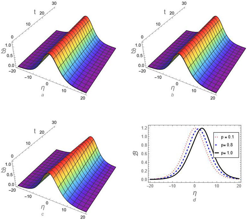
Figure 1. The profile of compressive ion-acoustic FKdV-soliton according to the approximation (46) is investigated against the fractional-order parameter $p$: (a) 3D-graph in the $\left(\eta ,t\right)$-plane for $p=0.1$, (b) 3D-graph in the $\left(\eta ,t\right)$-plane for $p=0.8$, (c) 3D-graph in the $\left(\eta ,t\right)$-plane for $p=1$, and (d) 2D-graph for $t=30$ and different values of $p$.

Figure 2

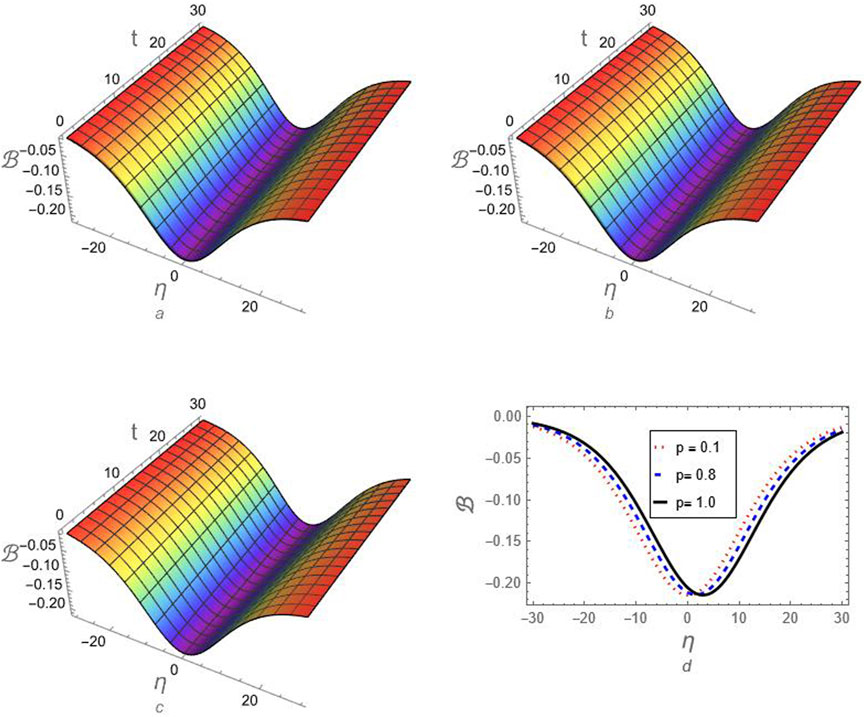
Figure 2. The profile of rarefactive ion-acoustic FKdV-soliton according to the approximation (46) is investigated against the fractional-order parameter $p$: (a) 3D-graph in the $\left(\eta ,t\right)$-plane for $p=0.1$, (b) 3D-graph in the $\left(\eta ,t\right)$-plane for $p=0.8$, (c) 3D-graph in the $\left(\eta ,t\right)$-plane for $p=1$, and (d) 2D-graph for $t=30$ and different values of $p$.

Figure 3

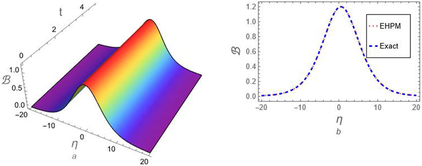
Figure 3. A comparison between the generated approximation (46) for compressive FKdV-soliton and the exact solution (32) at $p=1$, (a) 3D-graph for the two solutions in the $\left(\eta ,t\right)$-plane and (b) 2D-graph for the two solutions at $t=1$.

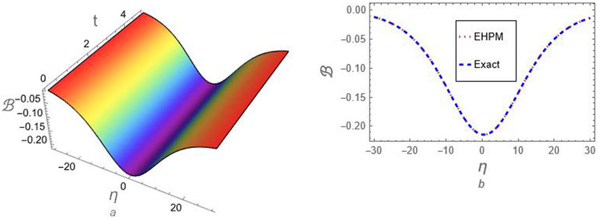
Figure 4

Figure 4. $1$, (a) 3D-graph for the two solutions in the $\left(\eta ,t\right)$-plane and (b) 2D-graph for the two solutions at $t=1$.

Table 1

Table 1. The absolute error for the generated approximations for compressive ion-acoustic FKdV-soliton is estimated at $\left(p,t\right)=\left(\mathrm{1,1}\right)$.

Table 2

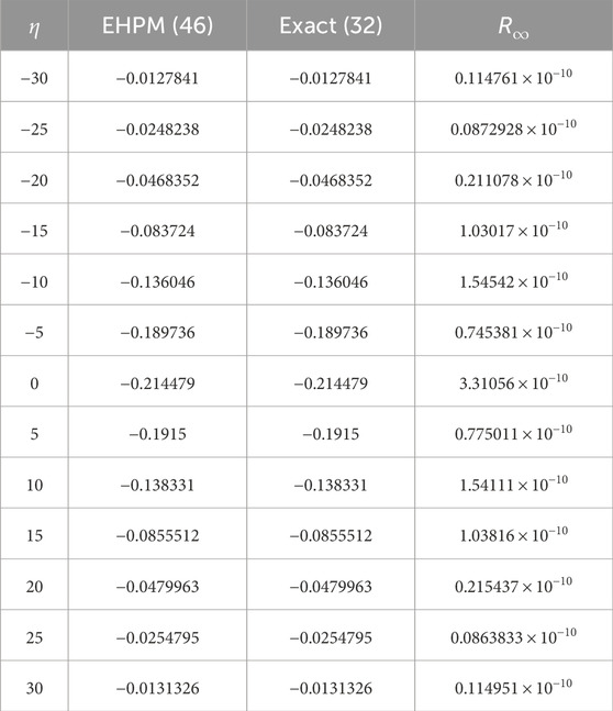
Table 2. The absolute error for the generated approximations for rarefactive ion-acoustic FKdV-soliton is estimated at $\left(p,t\right)=\left(\mathrm{1,1}\right)$.

4.3 Example (II): planar cubic nonlinear FmKdV equation

Here, we proceed to analyze the following planar cubic nonlinear FmKdV equation [70].

$D_t^p\mathcal{B}+C{\mathcal{B}}^2{\partial }_{\eta }\mathcal{B}+B{\partial }_{\eta }^3\mathcal{B}=0,\forall 0<p\le 1,(47)$

with IC

$\mathcal{B}\left(\eta ,0\right)\equiv {\mathcal{B}}_0=f,(48)$

where $f\equiv f\left(\eta \right)$ any IC for the planar integer mKdV, such as solitary and shock waves. For solitons to propagate in any plasma model or other physical system, the nonlinearity coefficient signal must be positive, i.e., $C>0$. Otherwise, i.e., for $C<0$, shock waves can propagate instead of solitons. Accordingly, the following IC for soliton is considered:

$f={\mathcal{B}}_{\max }\mathrm{s}\mathrm{e}\mathrm{c}\mathrm{h}\left(\frac{\eta }{w}\right),(49)$

which, the following exact soliton solution to Equation 47 for $C>0$ and $p=1$, is introduced

$\mathcal{B}={\mathcal{B}}_{\max }\mathrm{s}\mathrm{e}\mathrm{c}\mathrm{h}\left(\frac{\eta -u_{0}t}{w}\right),(50)$

where ${\mathcal{B}}_{\max }=\sqrt{6u_0/C}$ and $w=\sqrt{B/u_0}$ are, respectively, the peak KdV-soliton amplitude and width, while $u_0$ indicates the nonlinear wave velocity in the relative frame.

To derive the shock wave solution for Equation 47 in its integer case, we rewrite it in the following new form based on the negative sign of the cubic nonlinear coefficient $C$:

$D_t^p\mathcal{B}-C{\mathcal{B}}^2{\partial }_{\eta }\mathcal{B}+B{\partial }_{\eta }^3\mathcal{B}=0,\forall 0<p\le 1,(51)$

Note that we separate the negative sign from the nonlinearity coefficient; therefore, this coefficient must take positive values during the analysis.

Now, by applying tanh method to Equation 51, the following exact shock wave solution at $p=1$ is obtained

$\mathcal{B}={\mathcal{B}}_{\max }\tanh \left(\frac{\eta -u_{0}t}{w}\right),(52)$

where ${\mathcal{B}}_{\max }=\sqrt{3u_0/C}$ and $w=\sqrt{2B/u_0}$ are, respectively, the maximum amplitude of the mKdV-shock waves and $u_0$ indicates the nonlinear wave velocity in the relative frame. In this case, the following IC for the shock waves is introduced

$f={\mathcal{B}}_{\max }\tanh \left(\frac{\eta }{w}\right),(53)$

To analyze problems (47) and (51) using EHPM, we start from Equation 58 in addition to the following brief points:

Step 1: Applying ET on Equations 47, 51 yields

$E\left[D_t^p\mathcal{B}\right]=-E\left[\pm C{\mathcal{B}}^2{\partial }_{\eta }\mathcal{B}+B{\partial }_{\eta }^3\mathcal{B}\right]\text{,}(54)$

Note that the positive sign refers to Equation 47, which supports solitons, while the negative sign indicates Equation 51, which supports shock waves.

Step 2: Using ET to the Caputo FDO as given in Equation 11 in Equation 54, we have

$u^{-p}E\left[\mathcal{B}\right]-{\displaystyle \sum _{k=0}^{m-1}}{u}^{2-p+k}{\left.{\partial }_t^i\mathcal{B}\left(\eta ,t\right)\right|}_{t=0}=-E\left[\pm C{\mathcal{B}}^2{\partial }_{\eta }\mathcal{B}+B{\partial }_{\eta }^3\mathcal{B}\right]\text{,}(55)$

which leads to

$E\left[\mathcal{B}\right]={\displaystyle \sum _{k=0}^{m-1}}{u}^{2+k}{\left.{\partial }_t^i\mathcal{B}\left(\eta ,t\right)\right|}_{t=0}-E\left[\pm C{\mathcal{B}}^2{\partial }_{\eta }\mathcal{B}+B{\partial }_{\eta }^3\mathcal{B}\right],(56)$

or

$E\left[\mathcal{B}\right]=u^2{\mathcal{B}}_0\left(\eta \right)-u^{p}E\left[\pm C{\mathcal{B}}^2{\partial }_{\eta }\mathcal{B}+B{\partial }_{\eta }^3\mathcal{B}\right],(57)$

Step 3: Taking the inverse ET to Equation 57 yields

$\begin{array}{ll}\hfill \mathcal{B}& =E^{-1}\left[u^2{\mathcal{B}}_0\left(\eta \right)\right]-E^{-1}\left[u^{p}E\left[\pm C{\mathcal{B}}^2{\partial }_{\eta }\mathcal{B}+B{\partial }_{\eta }^3\mathcal{B}\right]\right]\hfill \\ \hfill & ={\mathcal{B}}_0\left(\eta \right)-E^{-1}\left[u^{p}E\left[\pm C{\mathcal{B}}^2{\partial }_{\eta }\mathcal{B}+B{\partial }_{\eta }^3\mathcal{B}\right]\right].\hfill \end{array}(58)$

Step 4: The approximate solution according to the HPM is denoted by the subsequent convergent series solution:

$\mathcal{B}={\displaystyle \sum _{m=0}^{\infty }}{\epsilon }^m{\mathcal{B}}_m,(59)$

where $\epsilon \in [\mathrm{0,1}]$ represents the homotopy parameter.

Step 5: In the following manner, the nonlinear term $\left(\pm C{\mathcal{B}}^2{\partial }_{\eta }\mathcal{B}\right)$ is decomposed

$\pm C{\mathcal{B}}^2{\partial }_{\eta }\mathcal{B}={\displaystyle \sum _{m=0}^{\infty }}{\epsilon }^m{H}_m\left(\mathcal{B}\right),(60)$

where $H_m\left(\mathcal{B}\right)$ indicates He’s polynomials and it is defined by

$H_m\left(\mathcal{B}\right)=\frac{1}{m!}\frac{{\partial }^m}{\partial {\epsilon }^m}{\left[\pm C{\left({\displaystyle \sum _{m=0}^{\infty }}{\epsilon }^m{\mathcal{B}}_m\right)}^2{\partial }_{\eta }\left({\displaystyle \sum _{m=0}^{\infty }}{\epsilon }^m{\mathcal{B}}_m\right)\right]}_{\epsilon =0},$

which leads to

$\begin{array}{ll}\hfill H_0\left(\mathcal{B}\right)& =\pm C{\mathcal{B}}_0^2{\partial }_{\eta }{\mathcal{B}}_0,\hfill \\ \hfill H_1\left(\mathcal{B}\right)& =\pm C\left({\mathcal{B}}_0^2{\partial }_{\eta }{\mathcal{B}}_1+2{\mathcal{B}}_0{\mathcal{B}}_1{\partial }_{\eta }{\mathcal{B}}_0\right),\hfill \\ \hfill H_2\left(\mathcal{B}\right)& =\pm C\left({\mathcal{B}}_0^2{\partial }_{\eta }{\mathcal{B}}_2+2{\mathcal{B}}_0{\mathcal{B}}_1{\partial }_{\eta }{\mathcal{B}}_1+\left({\mathcal{B}}_1^2+2{\mathcal{B}}_0{\mathcal{B}}_2\right){\partial }_{\eta }{\mathcal{B}}_0\right),\hfill \\ \hfill H_3\left(\mathcal{B}\right)& =\pm C\left({\mathcal{B}}_0^2{\partial }_{\eta }{\mathcal{B}}_3+2{\mathcal{B}}_0{\mathcal{B}}_1{\partial }_{\eta }{\mathcal{B}}_2+\left({\mathcal{B}}_1^2+2{\mathcal{B}}_0{\mathcal{B}}_2\right){\partial }_{\eta }{\mathcal{B}}_1+2\left({\mathcal{B}}_0{\mathcal{B}}_3+{\mathcal{B}}_1{\mathcal{B}}_2\right){\partial }_{\eta }{\mathcal{B}}_0\right),\hfill \\ \hfill & ⋮.\hfill \end{array}$

Step 6: Inserting Equations 59, 60 into Equation 58 yields

${\displaystyle \sum _{m=0}^{\infty }}{\epsilon }^m{\mathcal{B}}_m={\mathcal{B}}_0\left(\eta \right)-\epsilon E^{-1}\left[u^{p}E\left[B{\partial }_{\eta }^3\left({\displaystyle \sum _{m=0}^{\infty }}{\epsilon }^m{\mathcal{B}}_m\right)+{\displaystyle \sum _{m=0}^{\infty }}{\epsilon }^m{H}_m\left(\mathcal{B}\right)\right]\right].(61)$

Step 7: Collecting the coefficients of various order of $\epsilon$, we get the following the following successive approximations:

• For $O\left({\epsilon }^0\right)$, the zeroth-order approximation is obtained as follows:

${\mathcal{B}}_0={\mathcal{B}}_0\left(\eta ,0\right)=f.(62)$

By considering the ICs for the solitary and shock waves as given in Equations 49, 53, respectively, we can get the explicit values for the zeroth-order approximations to the two nonlinear structures:

${\left.{\mathcal{B}}_0\right|}_{\text{Solitons}}={\mathcal{B}}_{\max }\mathrm{s}\mathrm{e}\mathrm{c}\mathrm{h}\left(\frac{\eta }{w}\right),(63)$

${\left.{\mathcal{B}}_0\right|}_{\text{Shocks}}={\mathcal{B}}_{\max }\tanh \left(\frac{\eta }{w}\right).(64)$

• For $O\left(\epsilon \right)$, the $1^{st}-$order approximation is obtained as follows:

${\mathcal{B}}_1=-E^{-1}\left[u^{p}E\left[B{\partial }_{\eta }^3{\mathcal{B}}_0+H_0\left(\mathcal{B}\right)\right]\right]=-\left(\pm C{f}^2{f}^{\prime }+B{f}^{\left(3\right)}\right)\frac{t^p}{\mathrm{\Gamma }\left(p+1\right)}.(65)$

By considering the ICs for the solitary and shock waves as given in Equations 49, 53, respectively, we can get the explicit values for the $1^{st}-$order approximations to the two nonlinear structures as follows:

${\left.{\mathcal{B}}_1\right|}_{\text{Solitons}}=\frac{{\mathcal{B}}_{\max }{Q}_1\tanh \left(\frac{\eta }{w}\right){\mathrm{s}\mathrm{e}\mathrm{c}\mathrm{h}}^3\left(\frac{\eta }{w}\right)}{2w^3}\frac{t^p}{\mathrm{\Gamma }\left(p+1\right)},(66)$

${\left.{\mathcal{B}}_1\right|}_{\text{Shocks}}=\frac{{\mathcal{B}}_{\max }{R}_1{\mathrm{s}\mathrm{e}\mathrm{c}\mathrm{h}}^4\left(\frac{\eta }{w}\right)}{w^3}\frac{t^p}{\mathrm{\Gamma }\left(p+1\right)},(67)$

with

$\begin{array}{ll}\hfill Q_1& =\left[B\left(\cosh \left(2\frac{\eta }{w}\right)-11\right)+2C{w}^2{\mathcal{B}}_{\max }^2\right],\hfill \\ \hfill R_1& =\left[-2B\left(\cosh \left(2\frac{\eta }{w}\right)-2\right)+C{w}^2{\mathcal{B}}_{\max }^2{\sinh }^2\left(\frac{\eta }{w}\right)\right].\hfill \end{array}$

• For $O\left({\epsilon }^2\right)$, the $2^{nd}-$order approximation is obtained as follows:

$\begin{array}{ll}\hfill {\mathcal{B}}_2& =-E^{-1}\left[u^{p}E\left[B{\partial }_{\eta }^3{\mathcal{B}}_1+H_1\left(\mathcal{B}\right)\right]\right]\hfill \\ \hfill & =\left[\begin{array}{c}\hfill \pm 2BCf\left(3{\left(f^{\prime \prime }\right)}^2+5f^{\prime }{f}^{\left(3\right)}\right)\hfill \\ \hfill +B\left(\pm 12C{\left(f^{\prime }\right)}^2{f}^{\prime \prime }+B{f}^{\left(6\right)}\right)\hfill \\ \hfill +4C^2{f}^3{\left(f^{\prime }\right)}^2+C^2{f}^4{f}^{\prime \prime }\pm 2BC{f}^2{f}^{\left(4\right)}\hfill \end{array}\right]\frac{t^{2p}}{\mathrm{\Gamma }\left(2p+1\right)}.\hfill \end{array}(68)$

By considering the ICs for the solitary and shock waves as given in Equations 49, 53, respectively, we can get the explicit values for the $2^{nd}-$order approximations to the two nonlinear structures as follows:

${\left.{\mathcal{B}}_2\right|}_{\text{Solitons}}=\frac{{\mathcal{B}}_{\max }{Q}_2{\mathrm{s}\mathrm{e}\mathrm{c}\mathrm{h}}^7\left(\frac{\eta }{w}\right)}{32w^6}\frac{t^{2p}}{\mathrm{\Gamma }\left(2p+1\right)},(69)$

${\left.{\mathcal{B}}_2\right|}_{\text{Shocks}}=-\frac{{\mathcal{B}}_{\max }{R}_2\tanh \left(\frac{\eta }{w}\right){\mathrm{s}\mathrm{e}\mathrm{c}\mathrm{h}}^6\left(\frac{\eta }{w}\right)}{w^6}\frac{t^{2p}}{\mathrm{\Gamma }\left(2p+1\right)},(70)$

with

$\begin{array}{ll}\hfill Q_2& =\left(8C{w}^2{\mathcal{B}}_{\max }^2{S}_1+S_2\right),\hfill \\ \hfill R_2& =\left(-2BC{w}^2{\mathcal{B}}_{\max }^2{J}_1+C^2{w}^4{\mathcal{B}}_{\max }^4{J}_2+J_3\right),\hfill \end{array}$

where the coefficients $S_1$, $S_2$, $J_1$, $J_2$, and $J_3$, are given in Supplementary Appendix SII.

• For $O\left({\epsilon }^3\right)$, the $3^{rd}-$order approximation is obtained as follows:

${\mathcal{B}}_3=-E^{-1}\left[u^{p}E\left[B{\partial }_{\eta }^3{\mathcal{B}}_2+H_2\left(\mathcal{B}\right)\right]\right]=-\left({\displaystyle \sum _{i=1}^6}{Y}_i\right)\frac{t^{3p}}{\mathrm{\Gamma }{\left(p+1\right)}^2\mathrm{\Gamma }\left(3p+1\right)},(71)$

where the coefficients $Y_1-Y_6$ are given in Supplementary Appendix SIII.By considering the ICs for the solitary and shock waves as given in Equations 49, 53, respectively, we can get the explicit values for the $1^{st}-$order approximations to the two nonlinear structures as follows:

${\left.{\mathcal{B}}_3\right|}_{\text{Solitons}}=\frac{{\mathcal{B}}_{\max }{Q}_3\tanh \left(\frac{\eta }{w}\right){\mathrm{s}\mathrm{e}\mathrm{c}\mathrm{h}}^9\left(\frac{\eta }{w}\right)}{128w^9}\frac{t^{3p}}{\mathrm{\Gamma }{\left(p+1\right)}^2\mathrm{\Gamma }\left(3p+1\right)},(72)$

${\left.{\mathcal{B}}_3\right|}_{\text{Shocks}}=-\frac{{\mathcal{B}}_{\max }{R}_3{\mathrm{s}\mathrm{e}\mathrm{c}\mathrm{h}}^{10}\left(\frac{\eta }{w}\right)}{8w^9}\frac{t^{3p}}{\mathrm{\Gamma }{\left(p+1\right)}^2\mathrm{\Gamma }\left(3p+1\right)},(73)$

with

$\begin{array}{ll}\hfill Q_3& =\left\{4C{w}^2{\mathcal{B}}_{\max }^2\left[B^2\left(S_3+S_4\right)+4C{w}^2{\mathcal{B}}_{\max }^2\left(S_5+S_6+S_7\right)\right]+B^3\mathrm{\Gamma }{\left(p+1\right)}^2{S}_8\right\},\hfill \\ \hfill R_3& =\left\{J_4+C{w}^2{\mathcal{B}}_{\max }^2\left(4B^2\left(J_5+J_6\right)+C{w}^2{\mathcal{B}}_{\max }^2\left(J_7+J_8+J_9\right)\right)\right\},\hfill \end{array}$

where the coefficients $S_3$-$S_8$ and $J_4$-$J_9$, are given in Supplementary Appendix SIV.

Step 8: For $\epsilon \to 1$, the following convergent approximate solutions in finite series form up to the third-order approximation are obtained:

• Soliton solution up to $3^{rd}-$order approximation:

$\begin{array}{ll}\hfill \mathcal{B}& ={\mathcal{B}}_0+{\mathcal{B}}_1+{\mathcal{B}}_2+{\mathcal{B}}_3\hfill \\ \hfill & ={\mathcal{B}}_{\max }\mathrm{s}\mathrm{e}\mathrm{c}\mathrm{h}\left(\frac{\eta }{w}\right)+\frac{{\mathcal{B}}_{\max }{Q}_1\tanh \left(\frac{\eta }{w}\right){\mathrm{s}\mathrm{e}\mathrm{c}\mathrm{h}}^3\left(\frac{\eta }{w}\right)}{2w^3}\frac{t^p}{\mathrm{\Gamma }\left(p+1\right)}\hfill \\ \hfill & +\frac{{\mathcal{B}}_{\max }{Q}_2{\mathrm{s}\mathrm{e}\mathrm{c}\mathrm{h}}^7\left(\frac{\eta }{w}\right)}{32w^6}\frac{t^{2p}}{\mathrm{\Gamma }\left(2p+1\right)}\hfill \\ \hfill & +\frac{{\mathcal{B}}_{\max }{Q}_3\tanh \left(\frac{\eta }{w}\right){\mathrm{s}\mathrm{e}\mathrm{c}\mathrm{h}}^9\left(\frac{\eta }{w}\right)}{128w^9}\frac{t^{3p}}{\mathrm{\Gamma }{\left(p+1\right)}^2\mathrm{\Gamma }\left(3p+1\right)}.\hfill \end{array}(74)$

• Shock wave solution up to $3^{rd}-$order approximation:

$\begin{array}{ll}\hfill \mathcal{B}& ={\mathcal{B}}_0+{\mathcal{B}}_1+{\mathcal{B}}_2+{\mathcal{B}}_3\hfill \\ \hfill & ={\mathcal{B}}_{\max }\tanh \left(\frac{\eta }{w}\right)+\frac{{\mathcal{B}}_{\max }{R}_1{\mathrm{s}\mathrm{e}\mathrm{c}\mathrm{h}}^4\left(\frac{\eta }{w}\right)}{w^3}\frac{t^p}{\mathrm{\Gamma }\left(p+1\right)}\hfill \\ \hfill & -\frac{{\mathcal{B}}_{\max }{R}_2\tanh \left(\frac{\eta }{w}\right){\mathrm{s}\mathrm{e}\mathrm{c}\mathrm{h}}^6\left(\frac{\eta }{w}\right)}{w^6}\frac{t^{2p}}{\mathrm{\Gamma }\left(2p+1\right)}\hfill \\ \hfill & -\frac{{\mathcal{B}}_{\max }{R}_3{\mathrm{s}\mathrm{e}\mathrm{c}\mathrm{h}}^{10}\left(\frac{\eta }{w}\right)}{8w^9}\frac{t^{3p}}{\mathrm{\Gamma }{\left(p+1\right)}^2\mathrm{\Gamma }\left(3p+1\right)}.\hfill \end{array}(75)$

It is clear that the generated soliton approximation (74) using EHPM is identical to the derived soliton approximation using the Tantawy technique, as discussed in Refs. [27].

To investigate how fractionality affects the dynamics of the ion-acoustic FmKdV-solitons in the current plasma model, the value of the nonextensive parameter is considered: $q=0.95$, which leads to $\left(C,B\right)=\left(0.359292,1.1968\right)$. The generated soliton approximation (74) is analyzed at different values of the fractionality $p$ to examine the impact of fractionality on the behavior and dynamics of ion-acoustic FmKdV-solitons that emerge and propagate inside the plasma model under consideration, as illustrated in Figure 5. This graphic illustrates how fractionality impacts the propagation dynamics of FmKdV-solitons in various physical systems, particularly in plasma physics. Additionally, we compared the derived FmKdV-soliton approximation (74) with the exact mKdV-soliton solution (50) for the integer case, as depicted in Figure 6, to validate the accuracy of the generated approximations. Moreover, the absolute error of the generated FmKdV-soliton approximation is numerically calculated, as shown in Table 3. The analysis results demonstrate the effectiveness of the methods employed in examining diverse, strong nonlinearity EWEs and producing high-precision approximations.

Figure 5

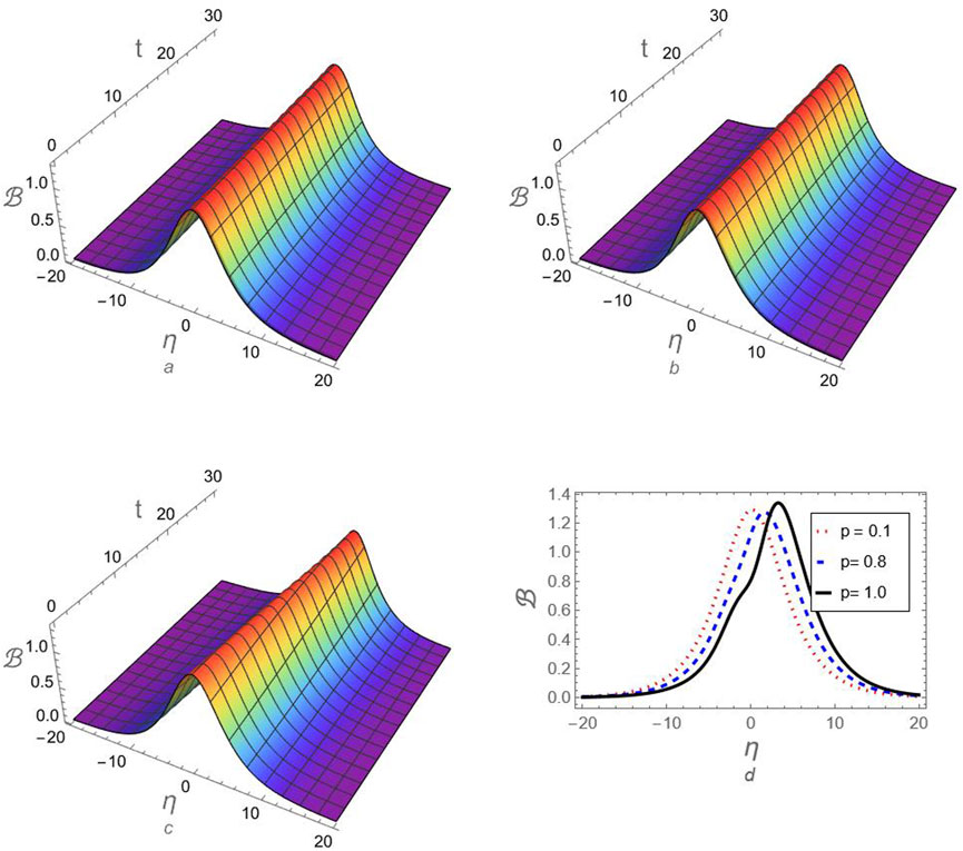
Figure 5. The profile of compressive ion-acoustic FmKdV-soliton according to the approximation (74) is investigated against the fractional-order parameter $p$: (a) 3D-graph in the $\left(\eta ,t\right)$-plane for $p=0.1$, (b) 3D-graph in the $\left(\eta ,t\right)$-plane for $p=0.8$, (c) 3D-graph in the $\left(\eta ,t\right)$-plane for $p=1$, and (d) 2D-graph for $t=30$ and different values of $p$.

Figure 6

Figure 6. A comparison between the generated approximation (74) for compressive FmKdV-soliton and the exact solution (50) at $p=1$, (a) 3D-graph for the two solutions in the $\left(\eta ,t\right)$-plane and (b) 2D-graph for the two solutions at $t=1$.

Table 3

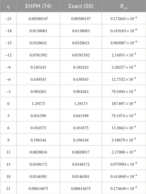
Table 3. The absolute error for the generated approximations for compressive ion-acoustic FmKdV-soliton is estimated at $\left(p,t\right)=\left(\mathrm{1,1}\right)$.

The profile of the fractional compressive FmKdV-shock waves according to the generated approximation (75) is examined against the fractional parameter $p$ as elucidated in Figure 7. We also presented a comparison between both the derived fractional compressive FmKdV-shock wave approximation (75) and the exact shock wave solution (52) at $p=1$, as shown in Figure 8, to verify the accuracy and stability of the derived approximations along the whole study domain. Furthermore, the absolute error of the compressive and rarefactive FmKdV-shock wave approximation (75) is estimated as shown in Tables 3, 4, respectively.

Figure 7

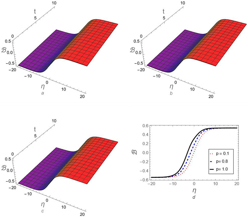
Figure 7. The profile of compressive FmKdV-shock waves according to the approximation (75) is investigated against the fractional-order parameter $p$: (a) 3D-graph in the $\left(\eta ,t\right)$-plane for $p=0.1$, (b) 3D-graph in the $\left(\eta ,t\right)$-plane for $p=0.8$, (c) 3D-graph in the $\left(\eta ,t\right)$-plane for $p=1$, and (d) 2D-graph for $t=30$ and different values of $p$.

Figure 8

Figure 8. A comparison between the generated approximation (75) for compressive FmKdV-shock waves and the exact solution (52) at $p=1$, (a) 3D-graph for the two solutions in the $\left(\eta ,t\right)$-plane and (b) 2D-graph for the two solutions at $t=1$.

Table 4

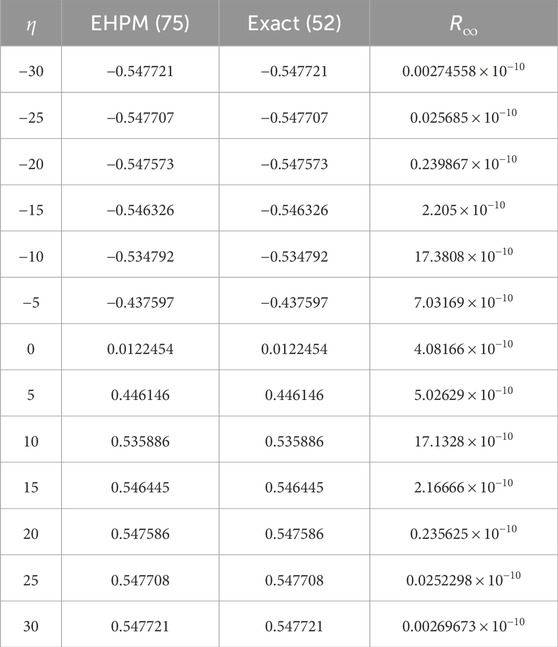
Table 4. The absolute error for the generated approximations for compressive FmKdV-shock waves is estimated at $\left(p,t\right)=\left(\mathrm{1,1}\right)$and $\left(B,C\right)=(\mathrm{1,1})$.

5 Conclusion

In this study, two of the most fundamental nonlinear evolutionary wave equations, which are widely used in various physical and engineering applications, have been analyzed. These equations are called the nonlinear planar fractional KdV (FKdV) and fractional modified KdV (FmKdV) equations, and they examined using Elzaki homotopy perturbation method (EHPM). For the quadratic nonlinear planar FKdV equation, a general formula up to the third order has been derived as a function of initial condition. After that, the soliton solution has been used as an initial solution, and an analytical fractional soliton approximation up to the third order has been generated. On the other hand, the cubic nonlinear planar FmKdV equation was divided into two parts: For the first part, if the cubic nonlinearity coefficient is positive, in this case, the FmKdV equation supports solitons and does not support shock waves. For this case, a general formula has been derived using the proposed approach as a function of initial condition. Subsequently, the soliton solution has been used as an initial solution, and an analytical fractional soliton approximation has been derived up to the third order. For the second form of the cubic nonlinear planar FmKdV equation, if the cubic nonlinearity coefficient is negative, in this case, the FmKdV equation does not support solitons, but rather shock waves. Using the proposed technique, a general formula has been derived as a function of initial condition. As a practical application to the obtained results, the fluid-governed equations for a collisionless and unmagnetized plasma composed of inertial cold ions and inertialess Cairns-Tsallis distributed electrons have been reduced to both the FKdV and FmKdV equations. After that, the effect of the fractional parameter on the dynamic behavior of the propagation of ion-acoustic waves in the plasma model under study has been investigated. We also performed a graphical comparison between all derived approximations and the exact solutions for the integer cases, i.e., at $p=1$, showing complete agreement between all derived approximations and the counterpart exact solutions. We also computed the absolute error for all derived approximations and found that they demonstrate good accuracy, thereby enhancing the effectiveness of the employed technique.

The derived approximations demonstrated that the provided approach can successfully and precisely solve problems with strong nonlinearity. We may conclude from the results that the used method is accurate in simulating the nonlinear structures (solitons and shock waves) in plasma physics and other scientific fields. The suggested results provide a comprehensive and valuable examination of the behavior of these waves. Several authors, particularly those working in nonlinear sciences, can benefit from the results in evaluating and interpreting their experimental and observational data.

6 Future work

This investigation has examined both the nonlinear planar FKdV and FmKdV equations. However, in numerous instances, the nonplanar and damped cases are more realistic for describing nonlinear phenomena in various plasma models. Consequently, in forthcoming studies, we will apply the two proposed approaches, in addition to the Tantawy technique [25–28], to analyze various nonlinear fractional EWEs that are extensively utilized in modeling numerous nonlinear phenomena in different plasma models, such as the nonplanar/damped FKdV-type equations [82, 83], the nonplanar/damped fractional Kawahara-type equations [84–87], the nonplanar/damped fractional Schrödinger-type equations [88–90], etc.

Data availability statement

The raw data supporting the conclusions of this article will be made available by the authors, without undue reservation.

Author contributions

WA: Formal Analysis, Investigation, Methodology, Writing – review and editing. AK: Investigation, Methodology, Writing – original draft. AA-J: Formal Analysis, Supervision, Validation, Writing – review and editing. SE-T: Formal Analysis, Investigation, Methodology, Software, Supervision, Writing – review and editing.

Funding

The author(s) declare that financial support was received for the research and/or publication of this article. The authors express their gratitude to Princess Nourah bint Abdulrahman University Researchers Supporting Project number (PNURSP2025R229), Princess Nourah bint Abdulrahman University, Riyadh, Saudi Arabia.

Acknowledgments

The authors express their gratitude to Princess Nourah bint Abdulrahman University Researchers Supporting Project number (PNURSP2025R229), Princess Nourah bint Abdulrahman University, Riyadh, Saudi Arabia.

Conflict of interest

The authors declare that the research was conducted in the absence of any commercial or financial relationships that could be construed as a potential conflict of interest.

Generative AI statement

The author(s) declare that no Generative AI was used in the creation of this manuscript.

Publisher’s note

All claims expressed in this article are solely those of the authors and do not necessarily represent those of their affiliated organizations, or those of the publisher, the editors and the reviewers. Any product that may be evaluated in this article, or claim that may be made by its manufacturer, is not guaranteed or endorsed by the publisher.

Supplementary material

The Supplementary Material for this article can be found online at: https://www.frontiersin.org/articles/10.3389/fphy.2025.1604640/full#supplementary-material

References

1. Ebaid A, Al-Jeaid HK. The mittag–leffler functions for a class of first-order fractional initial value problems: dual solution via riemann–liouville fractional derivative. Fractal Fract (2022) 6(2):85. doi:10.3390/fractalfract6020085

CrossRef Full Text | Google Scholar

2. Ait Touchent K, Hammouch Z, Mekkaoui T, Belgacem FB. Implementation and convergence analysis of homotopy perturbation coupled with Sumudu transform to construct solutions of local-fractional PDEs. Fractal and Fractional (2018) 2(3):22. doi:10.3390/fractalfract2030022

CrossRef Full Text | Google Scholar

3. Asif NA, Hammouch Z, Riaz MB, Bulut H. Analytical solution of a Maxwell fluid with slip effects in view of the Caputo-Fabrizio derivative. Eur Phys J Plus (2018) 133:272. doi:10.1140/epjp/i2018-12098-6

CrossRef Full Text | Google Scholar

4. Huang Q, Zhdanov R. Symmetries and exact solutions of the time fractional Harry-Dym equation with Riemann–Liouville derivative. Physica A: Stat Mech its Appl (2014) 409:110–8. doi:10.1016/j.physa.2014.04.043

CrossRef Full Text | Google Scholar

5. Alfadil H, Abouelregal AE, Marin M, Carrera E. Goufo-Caputo fractional viscoelastic photothermal model of an unbounded semiconductor material with a cylindrical cavity. Mech Adv Mater Structures (2024) 31(27):9625–38. doi:10.1080/15376494.2023.2278181

CrossRef Full Text | Google Scholar

6. Riaz MB, Imran MA, Shabbir K. Analytic solutions of Oldroyd-B fluid with fractional derivatives in a circular duct that applies a constant couple. Alexandria Eng J (2016) 55(4):3267–75. doi:10.1016/j.aej.2016.07.032

CrossRef Full Text | Google Scholar

7. Riaz MB, Zafar AA. Exact solutions for the blood flow through a circular tube under the influence of a magnetic field using fractional Caputo-Fabrizio derivatives. Math Model Nat Phenomena (2018) 13(1):8. doi:10.1051/mmnp/2018005

CrossRef Full Text | Google Scholar

8. Hilfer R. Applications of fractional calculus in physics. Singapore: World Scientific (2000).

Google Scholar

9. Kilbas AA, Srivastava HM, Trujillo JJ. Theory and applications of fractional differential equations, 204. Elsevier (2006).

Google Scholar

10. Mainardi F. Fractional calculus and waves in linear viscoelasticity: an introduction to mathematical models. World Scientific (2022). doi:10.1142/p614

CrossRef Full Text | Google Scholar

11. Miller KS, Ross B. An introduction to the fractional calculus and fractional differential equations. Wiley-Interscience (1993).

Google Scholar

12. Ebaid A, Cattani C, Al Juhani AS, El-Zahar ER. A novel exact solution for the fractional Ambartsumian equation. Adv Differ Equ (2021) 2021:88. doi:10.1186/s13662-021-03235-w

CrossRef Full Text | Google Scholar

13. Phaochoo P, Wisseksakwichai C, Thongpool N, Chankong S, Promluang K. Application of fractional derivative for the study of chemical reaction. Int J Intell Netw (2023) 13:2245.

Google Scholar

14. Aslam M, Farman M, Ahmad H, Gia TN, Ahmad A, Askar S. Fractal fractional derivative on chemistry kinetics hires problem. AIMS Mathematics (2021) 7(1):1155–84. doi:10.3934/math2022068

CrossRef Full Text | Google Scholar

15. Tang TQ, Jan R, Ahmad H, Shah Z, Vrinceanu N, Racheriu M. A fractional perspective on the dynamics of hiv, considering the interaction of viruses and immune system with the effect of antiretroviral therapy. J Nonlinear Math Phys (2023) 30(4):1327–44. doi:10.1007/s44198-023-00133-5

CrossRef Full Text | Google Scholar

16. Aljohani AF, Ebaid A, Algehyne EA, Mahrous YM, Cattani C, Al-Jeaid HK. The mittag-leffler function for Re-evaluating the chlorine transport model: comparative analysis. Fractal Fract (2022) 6(3):125. doi:10.3390/fractalfract6030125

CrossRef Full Text | Google Scholar

17. Alharbi WG, Shater AF, Ebaid A, Cattani C, Areshi M, Jalal MM, et al. Communicable disease model in view of fractional calculus. AIMS Mathematics (2023) 8(5):10033–48. doi:10.3934/math.2023508

CrossRef Full Text | Google Scholar

18. Sun H, Zhang Y, Baleanu D, Chen W, Chen Y. A new collection of real world applications of fractional calculus in science and engineering. Commun Nonlinear Sci Numer Simulation (2018) 64:213–31. doi:10.1016/j.cnsns.2018.04.019

CrossRef Full Text | Google Scholar

19. Beyer H, Kempfle S. Definition of physically consistent damping laws with fractional derivatives. ZAMM-Journal Appl Mathematics Mechanics/Zeitschrift für Angew Mathematik Mechanik (1995) 75(8):623–35. doi:10.1002/zamm.19950750820

CrossRef Full Text | Google Scholar

20. He JH. Approximate analytical solution for seepage flow with fractional derivatives in porous media. Computer Methods Appl Mech Eng (1998) 167(1-2):57–68. doi:10.1016/s0045-7825(98)00108-x

CrossRef Full Text | Google Scholar

21. Algehyne EA, Aldhabani MS, Areshi M, El-Zahar ER, Ebaid A, Al-Jeaid HK. A proposed application of fractional calculus on time dilation in special theory of relativity. Mathematics (2023) 11(15):3343. doi:10.3390/math11153343

CrossRef Full Text | Google Scholar

22. Sommacal L, Melchior P, Dossat A, Petit J, Cabelguen JM, Oustaloup A, et al. Improvement Muscle Fractional Multimodel Low-rate Stimulation. Biomed Signal Process Control (2007) 2(3):226–33. doi:10.1016/j.bspc.2007.07.013

CrossRef Full Text | Google Scholar

23. Silva MF, Machado JT, Lopes AM. Fractional order control of a hexapod robot. Nonlinear Dyn (2004) 38:417–33. doi:10.1007/s11071-004-3770-8

CrossRef Full Text | Google Scholar

24. Mathieu B, Melchior P, Oustaloup A, Ceyral C. Fractional differentiation for edge detection. Signal Process. (2003) 83(11):2421–32. doi:10.1016/s0165-1684(03)00194-4

CrossRef Full Text | Google Scholar

25. El-Tantawy SA, Al-Johani AS, Almuqrin AH, Khan A, El-Sherif LS. Novel approximations to the fourth-order fractional Cahn–Hillard equations: application to the Tantawy Technique and other two techniques with Yang transform. J Low Frequency Noise, Vibration Active Control (2025) 0(0). doi:10.1177/14613484251322240

CrossRef Full Text | Google Scholar

26. El-Tantawy SA, Bacha SIH, Khalid M, Alhejaili W. Application of the Tantawy technique for modeling fractional ion-acoustic waves in electronegative plasmas having Cairns distributed-electrons, Part (I): fractional KdV Solitary Waves. Braz J Phys (2025) 55:123. doi:10.1007/s13538-025-01741-w

CrossRef Full Text | Google Scholar

27. El-Tantawy SA, Alhejaili W, Khalid M, Al-Johani AS. Application of the Tantawy technique for modeling fractional ion-acoustic waves in electronegative nonthermal plasmas, part (II): fractional modified KdV-solitary waves. Braz J Phys (2025) 55:176. doi:10.1007/s13538-025-01800-2

CrossRef Full Text | Google Scholar

28. El-Tantawy SA, Khan D, Khan W, Khalid M, Alhejaili W. A novel approximation to the fractional KdV equation using the Tantawy technique and modeling fractional electron-acoustic cnoidal waves in a nonthermal plasma. Braz J Phys (2025) 55:163. doi:10.1007/s13538-025-01780-3

CrossRef Full Text | Google Scholar

29. Atangana A, Alkahtani BST. New model of groundwater flowing within a confine aquifer: application of Caputo-Fabrizio derivative. Arabian J Geosciences (2016) 9:8–6. doi:10.1007/s12517-015-2060-8

CrossRef Full Text | Google Scholar

30. Zureigat H, Ismail AI, Sathasivam S. Numerical solutions of fuzzy fractional diffusion equations by an implicit finite difference scheme. Neural Comput Appl (2019) 31:4085–94. doi:10.1007/s00521-017-3299-7

CrossRef Full Text | Google Scholar

31. Haider JA, Alhuthali AM, Elkotb MA. Exploring novel applications of stochastic differential equations: unraveling dynamics in plasma physics with the Tanh-Coth method. Results Phys (2024) 60:107684. doi:10.1016/j.rinp.2024.107684

CrossRef Full Text | Google Scholar

32. Guo P. The adomian decomposition method for a type of fractional differential equations. J Appl Mathematics Phys (2019) 7:2459–66. doi:10.4236/jamp.2019.710166

CrossRef Full Text | Google Scholar

33. Momani S. An explicit and numerical solutions of the fractional KdV equation. Mathematics Comput Simulation (2005) 70:110–8. doi:10.1016/j.matcom.2005.05.001

CrossRef Full Text | Google Scholar

34. Yang AM, Li J, Srivastava HM, Xie GN, Yang XJ. Local fractional Laplace variational iteration method for solving linear partial differential equations with local fractional derivative. Discrete Dyn Nat Soc (2014) 2014(1):365981–8. doi:10.1155/2014/365981

CrossRef Full Text | Google Scholar

35. Thirumalai S, Seshadri R. Spectral solutions of fractional differential equation modelling electrohydrodynamics flow in a cylindrical conduit. Commun Nonlinear Sci Numer Simulation (2019) 79:104931. doi:10.1016/j.cnsns.2019.104931

CrossRef Full Text | Google Scholar

36. Yousif AA, AbdulKhaleq FA, Mohsin AK, Mohammed OH, Malik AM. A developed technique of homotopy analysis method for solving nonlinear systems of Volterra integro-differential equations of fractional order. Partial Differential Equations Appl Mathematics (2023) 8:100548. doi:10.1016/j.padiff.2023.100548

CrossRef Full Text | Google Scholar

37. Hemeda AA. New iterative method: an application for solving fractional physical differential equations. Abstract Appl Anal (2013) 2013(1):1–9. doi:10.1155/2013/617010

CrossRef Full Text | Google Scholar

38. Alyousef HA, Shah R, Tiofack CGL, Salas AH, Alhejaili W, Ismaeel SME, et al. Novel approximations to the third- and fifth-order fractional KdV-type equations and modeling nonlinear structures in plasmas and fluids. Braz J Phys (2025) 55:20. doi:10.1007/s13538-024-01660-2

CrossRef Full Text | Google Scholar

39. Ibis B, Bayram M, Agargun AG. Applications of fractional differential transform method to fractional differential-algebraic equations. Eur J Pure Appl Mathematics (2011) 4(2):129–141.

Google Scholar

40. Moosavi Noori SR, Taghizadeh N. Modified differential transform method for solving linear and nonlinear pantograph type of differential and Volterra integro-differential equations with proportional delays. Adv Differ Equ (2020) 2020:649. doi:10.1186/s13662-020-03107-9

CrossRef Full Text | Google Scholar

41. Zhang J, Tian X. Laplace-residual power series method for solving fractional generalized long wave equations. Ocean Eng (2024) 310(2):118693. doi:10.1016/j.oceaneng.2024.118693

CrossRef Full Text | Google Scholar

42. Oqielat MN, Eriqa T, Ogilat O, El-Ajou A, Alhazmi SE, Al-Omari S. Laplace-residual power series method for solving time-fractional reaction–diffusion model. Fractal and Fractional (2023) 7(4):309. doi:10.3390/fractalfract7040309

CrossRef Full Text | Google Scholar

43. El-Tantawy SA, Matoog RT, Shah R, Alrowaily AW, Ismaeel SME. On the shock wave approximation to fractional generalized Burger–Fisher equations using the residual power series transform method. Phys Fluids (2024) 36(2):023105. doi:10.1063/5.0187127

CrossRef Full Text | Google Scholar

44. Oloniiju SD, Mukwevho N, Tijani YO, Otegbeye O. Chebyshev pseudospectral method for fractional differential equations in non-overlapping partitioned domains. AppliedMath (2024) 4:950–74. doi:10.3390/appliedmath4030051

CrossRef Full Text | Google Scholar

45. Amin R, Alshahrani B, Mahmoud M, Abdel-Aty A, Shah K, Deebani W. Haar wavelet method for solution of distributed order time-fractional differential equations. Alexandria Eng J (2021) 60(3):3295–303. doi:10.1016/j.aej.2021.01.039

CrossRef Full Text | Google Scholar

46. Wang Q. Homotopy perturbation method for fractional KdV equation. Appl Mathematics Comput (2007) 190:1795–802. doi:10.1016/j.amc.2007.02.065

CrossRef Full Text | Google Scholar

47. Wang Q. Homotopy perturbation method for fractional KdV-Burgers equation. Chaos, Solitons and Fractals (2008) 35:843–50. doi:10.1016/j.chaos.2006.05.074

CrossRef Full Text | Google Scholar

48. Alaje AI, Olayiwola MO, Adedokun KA, Adedeji JA, Oladapo AO. Modified homotopy perturbation method and its application to analytical solitons of fractional-order Korteweg–de Vries equation. Beni-suef Univ J Basic Appl Sci (2022) 11:139. doi:10.1186/s43088-022-00317-w

CrossRef Full Text | Google Scholar

49. Hemeda AA. Modified homotopy perturbation method for solving fractional differential equations. J Appl Mathematics (2014) 2014:1–9. doi:10.1155/2014/594245

CrossRef Full Text | Google Scholar

50. Abdulaziz O, Hashim I, Ismail ES. Approximate analytical solution to fractional modified KdV equations. Math Computer Model (2009) 49:136–45. doi:10.1016/j.mcm.2008.01.005

CrossRef Full Text | Google Scholar

51. Khirsariya SR, Rao SB, Chauhan JP. A novel hybrid technique to obtain the solution of generalized fractional-order differential equations. Mathematics Comput Simulation (2023) 205:272–90. doi:10.1016/j.matcom.2022.10.013

CrossRef Full Text | Google Scholar

52. Ganie AH, Mofarreh F, Khan A. On new computations of the time-fractional nonlinear KdV-Burgers equation with exponential memory. Physica Scripta (2024) 99(4):045217. doi:10.1088/1402-4896/ad2e60

CrossRef Full Text | Google Scholar

53. Sebastiano G, Pantano P, Tucci P. An electrical model for the Korteweg-de Vries equation. Am J Phys (1984) 52(3):238–43. doi:10.1119/1.13685

CrossRef Full Text | Google Scholar

54. Kengne E, Lakhssassi A, Liu W. Nonlinear Schamel–Korteweg deVries equation for a modified Noguchi nonlinear electric transmission network: analytical circuit modeling. Chaos Solitons Fractals (2020) 140:110229. doi:10.1016/j.chaos.2020.110229

CrossRef Full Text | Google Scholar

55. Ludu A, Ionescu RA, Greiner W. Generalized KdV equation for fluid dynamics and quantum algebras. Found Phys (1996) 26:665–78. doi:10.1007/bf02058238

CrossRef Full Text | Google Scholar

56. Ruggieri M, Speciale MP. KdV-like equations for fluid dynamics. AIP Conf Proc (2014) 1637:918–24. doi:10.1063/1.4904664

CrossRef Full Text | Google Scholar

57. Hereman W. Shallow water waves and solitary waves. In: R Meyers, editor. Mathematics of complexity and dynamical systems. New York, NY: Springer (2012). doi:10.1007/978-1-4614-1806-1_96

CrossRef Full Text | Google Scholar

58. Debnath L. Water waves and the Korteweg–de Vries equation. In: R Meyers, editor. Mathematics of complexity and dynamical systems. New York, NY: Springer (2012). doi:10.1007/978-1-4614-1806-1_113

CrossRef Full Text | Google Scholar

59. Wazwaz AM. Partial differential equations and solitary waves theory. Beijing: Higher Education Press (2009).

Google Scholar

60. Wazwaz AM. Partial differential equations: methods and applications. Lisse: Balkema, Cop (2002).

Google Scholar

61. Kashkari BS, El-Tantawy SA, Salas AH, El-Sherif LS. Homotopy perturbation method for studying dissipative nonplanar solitons in an electronegative complex plasma. Chaos Solitons Fractals (2020) 130:109457. doi:10.1016/j.chaos.2019.109457

CrossRef Full Text | Google Scholar

62. Almutlak SA, Parveen S, Mahmood S, Qamar A, Alotaibi BM, El-Tantawy SA. On the propagation of cnoidal wave and overtaking collision of slow shear Alfvén solitons in low β − magnetized plasmas. Phys Fluids (2023) 35:075130. doi:10.1063/5.0158292

CrossRef Full Text | Google Scholar

63. Alyousef HA, Khan D, Khan W, Khalid M, Tiofack CGL, El-Tantawy SA. Oblique propagation of high-frequency electron-acoustic periodic waves in a nonthermal plasma. AIP Adv (2025) 15:035040. doi:10.1063/5.0252686

CrossRef Full Text | Google Scholar

64. El-Tantawy SA. Nonlinear dynamics of soliton collisions in electronegative plasmas: the phase shifts of the planar KdV-and mkdV-soliton collisions. Chaos Solitons Fractals (2016) 93:93162–8. doi:10.1016/j.chaos.2016.10.011

CrossRef Full Text | Google Scholar

65. Albalawi W, El-Tantawy SA, Salas AH. On the rogue wave solution in the framework of a Korteweg–de Vries equation. Results Phys (2021) 30:104847. doi:10.1016/j.rinp.2021.104847

CrossRef Full Text | Google Scholar

66. Akbulut A, Taşcan F. Lie symmetries, symmetry reductions and conservation laws of time fractional modified Korteweg–de Vries (mkdv) equation. Chaos, Solitons and Fractals (2017) 100:1–6. doi:10.1016/j.chaos.2017.04.020

CrossRef Full Text | Google Scholar

67. Sahadevan R, Bakkyaraj T. Invariant analysis of time fractional generalized Burgers and Korteweg–de Vries equations. J Math Anal Appl (2012) 393(2):341–7. doi:10.1016/j.jmaa.2012.04.006

CrossRef Full Text | Google Scholar

68. Tribeche M, Amour R, Shukla PK. Ion acoustic solitary waves in a plasma with nonthermal electrons featuring Tsallis distribution. Phys Rev E (2012) 85:037401. doi:10.1103/physreve.85.037401

PubMed Abstract | CrossRef Full Text | Google Scholar

69. Williams G, Kourakis I, Verheest F, Hellberg MA. Re-examining the Cairns-Tsallis model for ion acoustic solitons. Phys Rev E (2013) 88:023103. doi:10.1103/physreve.88.023103

PubMed Abstract | CrossRef Full Text | Google Scholar

70. El-Tantawy SA, Wazwaz A-M, Schlickeiser R. Solitons collision and freak waves in a plasma with Cairns-Tsallis particle distributions. Plasma Phys Control Fusion (2015) 57:125012. doi:10.1088/0741-3335/57/12/125012

CrossRef Full Text | Google Scholar

71. Elzaki TM. The new integral transform Elzaki transform. Glob J Pure Appl Math (2011) 7(1):57–64.

Google Scholar

72. He JH. A coupling method of a homotopy technique and a perturbation technique for non-linear problems. Int J non-linear Mech (2000) 35(1):37–43. doi:10.1016/s0020-7462(98)00085-7

CrossRef Full Text | Google Scholar

73. He JH. Homotopy perturbation method: a new nonlinear analytical technique. Appl Mathematics Comput (2003) 135(1):73–9. doi:10.1016/s0096-3003(01)00312-5

CrossRef Full Text | Google Scholar

74. Mohamed MZ, Yousif M, Hamza AE. Solving nonlinear fractional partial differential equations using the Elzaki transform method and the homotopy perturbation method. Abstract Appl Anal (2022) 2022:1–9. doi:10.1155/2022/4743234

CrossRef Full Text | Google Scholar

75. Alshikh AA, Mahgob MMA. A comparative study between Laplace transform and two new integrals Elzaki transform and Aboodh transform. Pure Appl Math J (2016) 5(5):145–50. doi:10.11648/j.pamj.20160505.11

CrossRef Full Text | Google Scholar

76. Elzaki TM, Alkhateeb SA. Modification of Sumudu transform “Elzaki transform” and Adomian decomposition method. Appl Math Sci (2015) 9(13):603–11. doi:10.12988/ams.2015.411968

CrossRef Full Text | Google Scholar

77. Elzaki TM. On the connections between Laplace and Elzaki transforms. Adv Theor Appl Math (2011) 6(1):1–11.

Google Scholar

78. Sedeeg AKH. A coupling Elzaki transform and homotopy perturbation method for solving nonlinear fractional heat-like equations. Am J Math Comput Model (2016) 1:15–20. doi:10.11648/j.ajmcm.20160101.12

CrossRef Full Text | Google Scholar

79. El-Wakil SA, Abulwafa EM, Zahran MA, Mahmoud AA. Time-fractional KdV equation: formulation and solution using variational methods. Nonlinear Dyn (2011) 65:55–63. doi:10.1007/s11071-010-9873-5

CrossRef Full Text | Google Scholar

80. El-Wakil SA, Abulwafa EM, El-shewy EK, Mahmoud AA. Time-fractional KdV equation for electron-acoustic waves in plasma of cold electron and two different temperature isothermal ions. Astrophys Space Sci (2011) 333:269–76. doi:10.1007/s10509-011-0629-6

CrossRef Full Text | Google Scholar

81. El-Wakil SA, Abulwafa EM, El-shewy EK, Mahmoud AA. Ion-acoustic waves in unmagnetized collisionless weakly relativistic plasma of warm-ion and isothermal-electron using time-fractional KdV equation. Adv Space Res (2012) 49:1721–7. doi:10.1016/j.asr.2012.02.018

CrossRef Full Text | Google Scholar

82. Shan TM, Masood W, Siddiq M, Asghar S, Alotaibi BM, Ismaeel SME, et al. Bücklund transformation for analyzing a cylindrical Korteweg-de Vries equation and investigating multiple soliton solutions in a plasma. Phys Fluids (2023) 35:103105. doi:10.1063/5.0166075

CrossRef Full Text | Google Scholar

83. El-Tantawy SA, Wazwaz A-M. Anatomy of modified Korteweg–de Vries equation for studying the modulated envelope structures in non-Maxwellian dusty plasmas: freak waves and dark soliton collisions. Phy Plasmas (2018) 25:092105. doi:10.1063/1.5045247

CrossRef Full Text | Google Scholar

84. Alharthi MR, Alharbey RA, El-Tantawy SA. Novel analytical approximations to the nonplanar Kawahara equation and its plasma applications. Eur Phys J Plus (2022) 137:1172. doi:10.1140/epjp/s13360-022-03355-6

CrossRef Full Text | Google Scholar

85. El-Tantawy SA, El-Sherif LS, Bakry AM, Alhejaili W, Wazwaz A-M. On the analytical approximations to the nonplanar damped Kawahara equation: cnoidal and solitary waves and their energy. Phys Fluids (2022) 34:113103. doi:10.1063/5.0119630

CrossRef Full Text | Google Scholar

86. Ismaeel SME, Wazwaz A-M, Tag-Eldin E, El-Tantawy SA. Simulation studies on the dissipative modified Kawahara solitons in a complex plasma. Symmetry (2023) 15(1):57. doi:10.3390/sym15010057

CrossRef Full Text | Google Scholar

87. Alyousef HA, Salas AH, Matoog RT, El-Tantawy SA. On the analytical and numerical approximations to the forced damped Gardner Kawahara equation and modeling the nonlinear structures in a collisional plasma. Phys Fluids (2022) 34:103105. doi:10.1063/5.0109427

CrossRef Full Text | Google Scholar

88. El-Tantawy SA, Salas AH, Alharthi MR. On the analytical and numerical solutions of the linear damped NLSE for modeling dissipative freak waves and breathers in nonlinear and dispersive mediums: an application to a pair-ion plasma. Front Phys (2021) 9:580224. doi:10.3389/fphy.2021.580224

CrossRef Full Text | Google Scholar

89. El-Tantawy SA, Alharbey RA, H Salas A. Novel approximate analytical and numerical cylindrical rogue wave and breathers solutions: an application to electronegative plasma. Solitons and Fractals (2022) 155:111776. doi:10.1016/j.chaos.2021.111776

CrossRef Full Text | Google Scholar

90. El-Tantawy SA, Salas AH, Alyousef HA, Alharthi MR. Novel approximations to a nonplanar nonlinear Schrödinger equation and modeling nonplanar rogue waves/breathers in a complex plasma. Chaos, Solitons and Fractals (2022) 163:112612. doi:10.1016/j.chaos.2022.112612

CrossRef Full Text | Google Scholar