Heat and superdiffusive melting fronts in unsaturated porous media

When water is present in a medium with pore sizes in a range of approximately 10 nm, the corresponding freezing-point depression will cause long-range broadening of a melting front. Describing the freezing-point depression by the Gibbs–Thomson equation and the pore-size distribution by a power law, we derive a nonlinear diffusion equation for the fraction of melted water. This equation yields superdiffusive spreading of the melting front with a diffusion exponent, which is given by the spatial dimension and the exponent describing the pore size distribution. We derive this solution analytically from energy conservation in the limit where all the energy is consumed by the melting and explore the validity of this approximation numerically. Finally, we explore a geological application of the theory to the case of one-dimensional subsurface melting fronts in granular or soil systems. These fronts, which are produced by heating of the surface, spread at a superdiffusive rate and affect the subsurface to significantly larger depths than a system without the effects of freezing-point depression.

1 Introduction

Water residing in $\sim$ 10 nm pores will stay in the liquid state at temperatures well below the bulk freezing point. Such freezing-point depression is caused by the Gibbs–Thomson effect, which in a porous medium with a range of pore sizes, will cause residual amounts of liquid water in small pores while water in the larger pores freezes. The frozen state of a single pore is illustrated in Figure 1, where a pre-melted layer of liquid water is assumed to be present. The situation where pores of different sizes coexist is illustrated in Figure 2. Several experimental studies of the freezing-point depression in small pores have been carried out, showing that quantitatively, the effect depends on such factors as salinity [1], wetting properties [2], and the pore geometry [3–5].

Figure 1

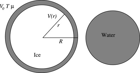
Figure 1. Left: A pore of total volume $V_0$ containing a liquid film and a core of ice. Right: A smaller pore containing liquid water at the same temperature.

Figure 2

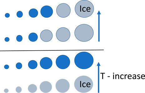
Figure 2. Pores containing water. Ice melting with (upper figure) and without (lower figure) the freezing-point depression. Ice is shown in gray, and liquid water is shown in blue.

The equilibrium states of frozen systems have been studied experimentally in both natural [1] and synthetic media, such as cylindrical silica nanopores [6] of controlled sizes in the 2–10 nm range. However, much less has been learned about the non-equilibrium processes of heat propagating through such systems, where only a fraction of the ice melts. When sufficient amounts of water are present at the right temperature, the energy required for this melting will dominate the energy balance; that is, the latent heat is larger than the energy needed to change the temperature due to the heat capacity. When different pore sizes are present, the heat may be consumed by melting only in a narrow range of these sizes (see Figure 2). This causes an increased spreading of the heat as well as the fraction $C$ of melted water. We will show that this fraction may spread in a superdiffusive manner when the pore size distribution is given by a power law. By comparison, a melting front in a medium where all the pores have the same size and melt at the same temperature will stop abruptly at the point in space where the available energy is consumed and thus has no long tail. Superdiffusion is characterized by the fact that the second spatial moment of the water fraction $C$ increases with time $t$ as $\sim t^{\tau }$ with the exponent $\tau >1/2$, the normal diffusion value being $\tau =1/2$. This behavior may arise in physical, biological, or geological systems; examples include Levy flights [7, 8], particle motion in random potentials, or the seemingly random paths of objects moving in turbulent flows [9, 10].

In addition to the shift in the equilibrium freezing point itself, there may be an effect of metastable states that cause superheating or supercooling. In order to address this question, we discuss qualitatively how the Gibbs–Thomson effect may be modified by nucleation barriers as well as the pore geometry and shapes of the ice. However, because the melting process is generally less affected by nucleation barriers and alternative nucleation pathways [3, 4, 11] than the freezing process, our theory is formulated for melting fronts and proceeds on the basis that metastable states may be neglected [12, 13].

We show that when the porous medium has a power law pore size distribution, the fraction of liquid water satisfies a non-linear diffusion equation. Solving this equation analytically, we proceed to demonstrate that this results in a superdiffusive, and, in some cases, even hyper-ballistic spreading of the heat and liquid concentration. The diffusion exponent is given in terms of the exponent governing the pore size distribution and the dimensionality.

These results may be of relevance for modeling melting in environments such as tundras. We therefore apply the model result to explore potential consequences for the depths at which the Gibbs–Thomson effect may affect the melting of ice in such contexts. Given the above assumptions, the depths at which the ice fraction is perturbed may be up to a factor 10 larger than without the effect of freezing-point depression. We also show numerically that this effect survives, even with realistic values for the energy consumed by the heat capacity of the water and the solid medium.

The article is organized as follows: In the theory section, we introduce the standard thermodynamics of the Gibbs–Thomson effect, deriving the expression for the freezing-point depression. Following the discussion of the equilibrium states, we discuss the assumption of a power law distribution for the pore sizes before we turn to the consequences for a time-dependent equation that governs the evolution of the melted water fraction and obtain its solutions in different spatial dimensions. Finally, we interpret these results in an assumed geological scenario where a melting front is caused by surface heating, which leads to a long-range, superdiffusive spreading of the melting front.

2 Theory

In the following, we obtain the volume fraction of liquid water as a function of temperature for a porous medium with a given pore size distribution and water/ice saturation $C_0$. For this purpose, we need the freezing point as a function of pore size.

It is a general fact that most water-bearing solids, or even ice itself [14], will have a pre-melted liquid layer [15, 16] of a thickness $\sim$nm, as illustrated in Figure 1. While the thickness of the melted films varies with the interaction energy between the water molecules and the walls [2], the existence of the film is quite insensitive to the corresponding wetting properties of the wall.

Being interested in pores on the nano- to micrometer scale, we will assume that the chemical potential $\mu$ is constant over the pores. This is justified by the fact that diffusion is fast on these scales, and so the water will quickly equilibrate to the chemical potential of the surroundings. This will be assumed to be the case whether the pore is open to the surrounding pore volume or not. The situation is illustrated in Figure 1. In this case, a body of ice will adjust its volume $V(r)$ so as to minimize the Landau, or grand canonical, potential $\mathrm{\Omega }$ in equilibrium. We will not consider the case where the increase in specific volume of the water during freezing leads to significant pressure changes. So, the theory is limited to the cases where there is some freedom for the water to expand or be absorbed, as is generally the case in unsaturated or unconsolidated porous media with boundaries that are open to the surroundings.

2.1 Freezing-point depression and the thermodynamics of the Gibbs–Thomson effect in spherical pores

The net energy effect of introducing a liquid layer between a solid (or vapor) and ice may be described by the Landau free energy

${\mathrm{\Omega }}_{VW}=A_0{A}_H/\left(12\pi d^2\right),(1)$

where $A_0$ is the surface area, and $d$ the liquid layer thickness. We have introduced the Hamaker constant $A_H\sim 10^{-20}-10^{-19}$ J (albeit with an unconventional sign to keep $A_H$ positive).

Adding the free energy of the ice–water interface $\sigma A(r)$, where $A(r)$ is the area of this interface and $\sigma$ is the ice–water surface energy per unit area, to the energy of the pre-melted layer given in Equation 1 yields the total free energy

$\mathrm{\Omega }=\sigma A+\frac{A_H{A}_0}{12\pi {\left(R-r\right)}^2}+{\mathrm{\Omega }}_0,(2)$

where the bulk free energy ${\mathrm{\Omega }}_0$ is independent of the interface contributions. Because in general $\mathrm{\Omega }=-PV$, the combined potential for both the liquid and ice is

${\mathrm{\Omega }}_0=-P_i{V}_i-P_w\left(V_0-V_i\right),(3)$

where the ice pressure $P_i$ and water pressure $P_w$ will in general differ.

At the bulk melting temperature $T_m=$ 273 K, there will be no change in ${\mathrm{\Omega }}_0$ under a change in $V_i$ when $\mu$ and $T$ are kept fixed, so, using the fact that ${\mathrm{\Omega }}_0=E-TS-\mu N$, we can write

$0=d{\mathrm{\Omega }}_0=dE-T_{m}dS-\mu dN(4)$

where $E$, $S$, and $N$ are the total ice–water energy, entropy, and molecule number, respectively. The heat needed to melt a volume $-d{V}_i$ of ice is ${\rho }_i\lambda d{V}_i$, where ${\rho }_i$ is the ice mass density and $\lambda$ is the latent heat per unit mass. Using this, the above equation may also be written

$-{\rho }_i\lambda d{V}_i=T_{m}dS=dE-\mu dN.(5)$

Because ${\rho }_i$ and $\lambda$ change very little over a modest temperature variation, we may also get $d{\mathrm{\Omega }}_0$ in the case where $T\ne T_m$ by writing

$\begin{array}{ll}\hfill d{\mathrm{\Omega }}_0& =\left(dE-\mu dN\right)-\frac{T}{T_m}{T}_{m}dS\hfill \\ \hfill & \approx -\left(1-\frac{T}{T_m}\right){\rho }_i\lambda d{V}_i,\hfill \end{array}(6)$

which indicates that the free energy change due to an ice volume increase is negative below the bulk freezing point. Integrating from $V_i=0$, where ${\mathrm{\Omega }}_o=-P_w(\mu ,T)V_0$, yields

${\mathrm{\Omega }}_0\approx -\left(1-\frac{T}{T_m}\right){\rho }_i\lambda V_i-P_w{V}_0,(7)$

which, when inserted in Equation 2, gives

$\mathrm{\Omega }=\sigma A+\frac{A_H{A}_0}{12\pi {\left(R-r\right)}^2}-\left(1-\frac{T}{T_m}\right){\rho }_i\lambda V_i-P_w{V}_0.(8)$

The change in this energy as $r$ is increased from $r=0$ is

$\mathrm{\Delta }\mathrm{\Omega }=\sigma A-\left(1-\frac{T}{T_m}\right){\rho }_i\lambda V_i+\frac{A_H}{12\pi }\left(\frac{A_0}{{\left(R-r\right)}^2}-\frac{A_0}{R^2}\right).(9)$

The equilibrium value of the ice radius is given by the global minimum of $\mathrm{\Delta }\mathrm{\Omega }$, which, for sufficiently small $R$ values, will be at $r=0$, that is, for the complete liquid state. Above this critical pore size, the minimum will be at $r_m\lesssim R$, a value that is given by the equilibrium thickness of the surface melted layer. As may be noted from Figure 3, this minimum does not change much with the pore size $R$. When $\mathrm{\Omega }(r=0)>\mathrm{\Omega }(r_m)$, there will still be ice. The condition for complete melting is that $\mathrm{\Omega }(r=0)<\mathrm{\Omega }(r_m)$, which yields the freezing-point depression.

Figure 3

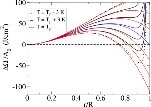
Figure 3. The Landau free energy per unit area in a pore of radius $R=10$ nm with a surface layer of water as a function of the radius $r$ of the ice volume at temperatures around $T_F=$ 264 K. The black curves show the free energy with $A_H=$ 10⁻²⁰ J, while the red curves show the free energy with $A_H=0$ J. For the blue curves, $T=T_F$.

Taking $r=R$, $A_H=0$ gives the free energy change in passing from a liquid to a fully frozen pore

$\mathrm{\Delta }\mathrm{\Omega }=\sigma A-\left(1-\frac{T}{T_m}\right){\rho }_i\lambda V_i,(10)$

where $A=4\pi R^2$ and $V_i=(4/3)\pi R^3$. The condition $\mathrm{\Delta }\mathrm{\Omega }=0$ implies that a pore of radius $R$ will freeze at a temperature $T=T_F$ given by

$T_F\left(R\right)=T_m\left(1-\frac{3\sigma }{{\rho }_i\lambda R}\right).(11)$

This is the standard expression for the Gibbs–Thomson effect. For a cylindrical pore, the geometrical factor of 3 must be replaced by 2. In the following, we shall use the value 3. Note that, due to the tendency of the surface tension to minimize the interface area, these smooth geometrical shapes will also be relevant in more complex pore geometries.

2.2 Corrections to the Gibbs–Thomson effect due to nucleation barriers

Thus far, we have ignored the time it takes for a metastable state to be replaced by the equilibrium state, implicitly assuming that the system has had time to reach the overall minimum state for the free energy. This is in general not the case as some metastable states may be very long-lived, a phenomenon that is quantified in classical nucleation theory [17, 18], which is based on the probability that a free energy barrier is traversed by the thermal activation energy $k_{B}T$. Moreover, the stability against melting may be very different from the stability against the reverse process of freezing. It is generally much more difficult to superheat a solid than to supercool a liquid [12, 13]. Superheated crystalline solids have only been observed in some rather singular cases where the heated region is along a single crystal plane or the crystals are confined inside a non-melting matrix [19, 20]. The existence of supercooled liquids, on the other hand, only requires the absence of nucleation sites.

Assuming our pre-melted surface layer of water, there is no extra energy cost (nucleation barrier) in forming a new liquid–ice surface during the melting process. Yet, there will be a nucleation barrier that must be crossed during melting when the temperature is $T\approx T_F$. The reason for this is that when melting happens around $T\approx T_F<T_m$, the bulk free energy must increase, while the surface energy is decreased. Thus, as $r$ decreases from a value around $R$ in Figure 3, the free energy initially increases. As a result, there is a free energy barrier against both melting and freezing. This fact implies the possible existence of solid ice that is superheated relative to its depressed freezing point $T_F$.

Using nucleation theory, it is possible to estimate the lifetime of these metastable states as $\propto \exp ((\mathrm{\Delta }\mathrm{\Omega }(r_{\mathit{max}})-\mathrm{\Delta }\mathrm{\Omega }(R))/(k_{B}T))$, where the free energy $\mathrm{\Delta }\mathrm{\Omega }(r)$ is shown in Figure 3 and takes its maximum at $r=r_{\mathit{max}}$. Requiring that the lifetime be within a realistic range, it is possible to show that the melting temperature must be increased above $T_F$ by an amount that corresponds to a reduction of the freezing-point depression $T_m-T_F$ by $\sim$ 20% for pore sizes greater than $\sim$ 1 nm.

It may be shown that nucleation barriers are significantly more influential during freezing (supercooled liquid). In this case, however, nucleation pathways other than ice forming as a spherical crystal are likely to dominate, as has been shown for the case where ice nucleates in pockets or corner geometries [3, 4, 11].

In the following, we will consider melting on the basis that metastable states may be neglected, although there is a nucleation barrier to be passed both for the melting and freezing transition in isolated pores. For melting, this assumption implies that there may be quantitative corrections to the depression $T_m-T_F$ by $\sim$ 20%, which are ignored.

2.3 Heat in a nanoporous medium with partially frozen water

Having dealt with the equilibrium problem of the freezing-point depression, we now investigate the non-equilibrium effects of this phenomenon in the context of a nanoporous material. We shall consider a melting front, for which the shift in melting temperature is small, and so the shift in the freezing-point depression will not be applied. Note, however, that a freezing front may differ significantly from the melting front through the possible existence of metastable pockets of supercooled liquid.

The pore size distributions may be estimated through nitrogen absorption [21], electron microscopy, or mercury injection experiments and measurements of the heat capacity variations with temperature when there is water present [22]. For silts, clays, and synthetic media made of glass powders [1], they may yield distributions that extend down at least to the nm scale. Freezing and melting of water confined in silica nanopores have been observed down to pore sizes of 3 nm [6].

The distributions may be given in terms of a relative volume fraction per unit length $g(R)$ so that $\int dRg(R)=\varphi$, the porosity of the medium. Our main assumption is that this distribution may be approximated with a power law above a minimum cut-off length $R_{\mathit{min}}$,

$g\left(R\right)=N{\left(R-R_{\mathit{min}}\right)}^{\beta }(12)$

where $N=(\beta +1)\varphi /{(R_{\mathit{max}}-R_{\mathit{min}})}^{\beta +1}$ is the normalization.

Mercury intrusion experiments are challenged by the fact that high injection pressures may crush or deform the smallest pores. Yet, in rigid materials, such as cement, the technique may be used to measure pores down to $R_{\mathit{min}}\sim$ 1 nm [23]. In order to cover the smaller pore ranges, nitrogen adsorption techniques are often better [21]. Zhao et al. [24] measured pore size distribution for porous sandstone from the Ordos basin by mercury injection, finding $g(R)$-distributions that are well described by $R_{\mathit{min}}\sim$ 10 nm and $\beta =1$ over 1 to 2 decades in pore sizes. Using ${\text{N}}_2$ adsorption techniques on porous glass powders, Fujinomori soil, and bentonite clay, Watanabe et al. [1] found $g(R)$-distributions where $R_{\mathit{min}}\approx$ 1 nm, $R_{\mathit{max}}\approx$ 3–4 nm, and $\beta =$ 1–2. Park et al. [25] measured pore-size distributions. Different sediments produced $R_{\mathit{min}}$ values from 1 nm to 100 nm with distributions that could be described by a $\beta \approx 2$ power law over roughly a decade. There is thus a range of natural and synthetic materials that seem to fulfill the assumed pore-size power law distribution over an adequate range of length scales.

In a medium that is described by Equation 12, all the pores are frozen when

$T=T_{\mathit{min}}=T_m-T_m\frac{r_0}{R_{\mathit{min}}},(13)$

where we have introduced the length $r_0=3\sigma /({\rho }_i\lambda )\approx 3.3$nm. Correspondingly, there is an upper temperature

$T_{\mathit{max}}=T_m-T_m\frac{r_0}{R_{\mathit{max}}},(14)$

where all pore water is melted.

The initial filling fraction of water in the pores $C_0$ gives the total water (ice or liquid) fraction $\varphi C_0$. The fraction of liquid water, $C(T)$, is the fraction contained in the pores that are so small that they have not frozen. These pores have sizes less than

$r\left(T\right)=\frac{3\sigma }{{\rho }_i\lambda \left(1-T/T_m\right)}.(15)$

This means that when $T_{\mathit{min}}<T<T_{\mathit{max}}$

$\begin{array}{ll}\hfill C\left(T\right)& =C_0{\int }_{R_{\mathit{min}}}^{r\left(T\right)}dRg\left(R\right)\hfill \\ \hfill & =N{C}_0{\int }_{R_{\mathit{min}}}^{r\left(T\right)}dR{\left(R-R_{\mathit{min}}\right)}^{\beta }\hfill \\ \hfill & =\frac{N{C}_0}{\beta +1}{\left(r\left(T\right)-R_{\mathit{min}}\right)}^{\beta +1}\hfill \end{array}(16)$

$=\frac{N{C}_0}{\left(\beta +1\right)}{R}_{\mathit{min}}^{\beta +1}{\left(\frac{T-T_{\mathit{min}}}{T_m-T}\right)}^{\beta +1},(17)$

by use of Equation 12 and Equation 13. Close to the absolute freezing point $T_{\mathit{min}}$, the above denominator is close to ${(T_m-T_{\mathit{min}})}^{\beta +1}$, so we shall use

$C\left(T\right)=B{\left(\frac{T-T_{\mathit{min}}}{T_{\mathit{min}}}\right)}^{\beta +1},(18)$

with

$B=C_0\varphi {\left(\frac{R_{\mathit{min}}^2}{R_{\mathit{max}}-R_{\mathit{min}}}\frac{{\rho }_i\lambda T_{\mathit{min}}}{3\sigma T_m}\right)}^{\beta +1}(19)$

by use of Equation 13 and the definition of $N$.

2.4 Contribution of pre-melted surface layers

Having neglected the thickness of the pre-melted films in the ice-filled pores by setting $A_H=0$, we should compare the relative contributions to $C(T)$ from these films and the liquid-filled pores. Because there is no film in the liquid-filled pores, we need only take the $R>r(T)$ pores into account. We take the film contribution to be given by the film thickness $d=R-r(T)$ as

$\mathrm{\Delta }C\left(T\right)=C_0{\int }_{r\left(T\right)}^{R_{\mathit{max}}}dRg\left(R\right)\frac{\mathrm{\Delta }V\left(R\right)}{V\left(R\right)},(20)$

where the fraction $\mathrm{\Delta }V/V\approx 3d/R$ is the ratio of the film volume to the pore volume. Then,

$\mathrm{\Delta }C\left(T\right)=3dN{C}_0{\int }_{r\left(T\right)}^{R_{\mathit{max}}}dR\frac{{\left(R-R_{\mathit{min}}\right)}^{\beta }}{R},(21)$

where $R_{\mathit{max}}$ is the upper cut-off for $g(R)$. When $\beta =1$, this integral is easily evaluated to give

$\mathrm{\Delta }C\left(T\right)=3d\left(T\right)N{C}_0\left(R_{\mathit{max}}-r\left(T\right)-R_{\mathit{min}}\ln \left(\frac{R_{\mathit{max}}}{r\left(T\right)}\right)\right).(22)$

Taking the $R_{\mathit{max}}$ term to dominate in this expression and using Equation 16, the ratio becomes

$\frac{\mathrm{\Delta }C}{C}\approx 6d\left(T\right)\frac{R_{\mathit{max}}}{{\left(r\left(T\right)-R_{\mathit{min}}\right)}^2},(23)$

which may well be larger than one when $r(T)\gtrsim R_{\mathit{min}}$.

However, as we shall see below, it is the rates of change $dC/dT$ of the volume fractions that are important, not the absolute value of $\mathrm{\Delta }C/C$. The film thickness $d$ may be estimated from Equation 9 as the minimum of $\mathrm{\Delta }\mathrm{\Omega }$ when $\sigma =0$. This gives the standard expression [16].

$d={\left(\frac{A_H{T}_m}{6\pi \left(T_m-T\right){\rho }_i\lambda }\right)}^{1/3},(24)$

where we can use the relatively high value $A_H=10^{-19}$ J. Together with the constants given in Table 1, this gives $d\approx$1 nm, while the other relevant length, which appears in Equation 9, is $3\sigma /({\rho }_i\lambda )\approx$ 0.3 nm.

Table 1

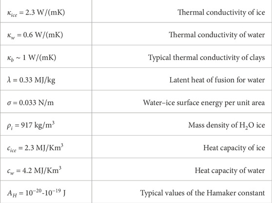
Table 1. Material constants.

Because $C\propto {(T-T_{\mathit{min}})}^2$ and, to leading order $\mathrm{\Delta }C\propto d\propto {(T-T_m)}^{-1/3}$, we have that $dC/dT=(\beta +1)C/(T-T_{\mathit{min}})$ while $d\mathrm{\Delta }C/dT=\mathrm{\Delta }C/(3(T_m-T))$, so that the ratio of the changes in these two quantities due to a temperature change when $\beta =1$ is

$\frac{\delta \mathrm{\Delta }C}{\delta C}=\frac{T_m}{T-T_{\mathit{min}}}\frac{d{r}_0{R}_{\mathit{max}}}{R_{\mathit{min}}^3}.(25)$

close to the absolute freezing point $T_{\mathit{min}}$. Here, we have used Equation 13 to substitute $(T_m-T_{\mathit{min}})/T_m=r_0/R_{\mathit{min}}$. The condition that $\delta \mathrm{\Delta }C/\delta C\ll 1$ may be taken as a condition on the range of pore sizes $R_{\mathit{max}}/R_{\mathit{min}}$:

$\frac{R_{\mathit{max}}}{R_{\mathit{min}}}\ll \frac{R_{\mathit{min}}^2}{d{r}_0}\frac{T-T_{\mathit{min}}}{T_m},(26)$

or, equivalently,

$\frac{T-T_{\mathit{min}}}{T_m-T_{\mathit{min}}}\gg \frac{d}{R_{\mathit{min}}}\frac{R_{\mathit{max}}}{R_{\mathit{min}}}.(27)$

When $R_{\mathit{min}}=$ 30 nm, for instance, and $(T-T_{\mathit{min}})/T_m=$ 1$/$273, we get that $R_{\mathit{max}}/R_{\mathit{min}}\ll 10$. It is quite natural that the condition for the domination of pore-versus film fluid is a limited range of pore sizes, as a domination of the large pores, which all carry a film contribution, would leave a smaller fraction of the porosity to be represented by smaller pores.

In other words, when $R_{\mathit{max}}/R_{\mathit{min}}\ll 10$, $\mathrm{\Delta }C$ changes relatively slowly with $T\approx T_{\mathit{min}}$, but $C$ changes significantly. In this case, we may neglect the variations in the film contribution to the overall change in liquid volume fraction. For this reason, we shall only use the $C$ in the following, keeping in mind that it is the fraction of liquid pore water, and not the total fraction of liquid water.

2.5 Governing equation for the evolution of melted water concentration

In a 1D setting, the conservation of energy in a slab of thickness $dx$ over a time $dt$ may be written

$\left(j\left(x\right)-j\left(x+dx\right)\right)\mathrm{\Delta }Adt=\lambda \rho \mathrm{\Delta }AdxdC+c_b\mathrm{\Delta }AdxdT(28)$

where $\mathrm{\Delta }A$ is the cross-sectional area, $c_b$ is the combined specific heat capacity of the porous medium and the water, and $T$ is the temperature. In Equation 28, the left-hand side is the net energy transfer to the slab, the first term on the right is the energy consumed by melting (latent heat), and the last term is the energy absorbed due to the heat capacities of the water, ice, and the porous medium itself. As $dx\to 0$, Equation 28 becomes

$\frac{\partial j}{\partial x}+\lambda \rho \frac{\partial C}{\partial t}+c_b\frac{\partial T}{\partial t}=0.(29)$

To describe the heat flow, we apply the Fourier law, which takes the form

$j=-\kappa \frac{\partial T}{\partial x},(30)$

where $\kappa$ is the bulk thermal conductivity of the porous medium, so inserting this in Equation 29 gives

$\frac{\partial }{\partial x}\left(\kappa \frac{\partial T}{\partial x}\right)=\left(\rho \lambda \frac{\partial C}{\partial T}+c_b\right)\frac{\partial T}{\partial t}(31)$

where we have used $\partial C/\partial t=(\partial C/\partial T)(\partial T/\partial t)$. Generalizing to arbitrary dimension $(\partial /\partial x\to \nabla )$ and replacing $T-T_{\mathit{min}}$ by $T_{\mathit{min}}{(C/B)}^{1/(\beta +1)}$ using Equation 18 yields the diffusion equation

$\left(1+M\right)\frac{\partial C}{\partial t}=D_0\nabla \cdot \left(C^{1/\left(\beta +1\right)-1}\nabla C\right).(32)$

where

$D_0=\frac{{\kappa }_b{T}_{\mathit{min}}}{\lambda \rho \left(\beta +1\right)B^{1/\left(\beta +1\right)}}=\frac{c_b{T}_{\mathit{min}}}{\lambda \rho \left(\beta +1\right)B^{1/\left(\beta +1\right)}}{D}_t,(33)$

and $D_t={\kappa }_b/c_b\approx$ ${1\text{mm}}^2/$s is the average thermal diffusivity of the porous medium, and

$\begin{array}{ll}\hfill M& =\frac{c_b{T}_{\mathit{min}}{C}^{1/\left(\beta +1\right)-1}}{\left(\beta +1\right){\rho }_i\lambda B^{1/\left(\beta +1\right)}}\hfill \\ \hfill & =\frac{3c_b\sigma T_m}{\left(\beta +1\right){\left({\rho }_i\lambda \right)}^2{\left(C_0\varphi \right)}^{1/\left(\beta +1\right)}}\frac{R_{\mathit{max}}-R_{\mathit{min}}}{R_{\mathit{min}}^2}{C}^{-\gamma }.\hfill \end{array}(34)$

The last expression comes from replacing $B$ by the expression in Equation 19, and $\gamma =\beta /(\beta +1)$. Using the material constants in Table 1 gives

$M=l\frac{R_{\mathit{max}}-R_{\mathit{min}}}{R_{\mathit{min}}^2}{C}^{-\gamma }(35)$

where $l\approx$ 0.4 nm. So $M\ll 1$ when the range of pore sizes is limited and as long as $C$ does not become too small.

We shall proceed to analyze the case where the $M$-term may be dropped, leaving the equation

$\frac{\partial C}{\partial t}=D_0\nabla \cdot \left(C^{-\gamma }\nabla C\right).(36)$

We note at this point that the condition for neglecting the energy needed to change temperature, which is represented by the $M$-term, coincides with the condition to neglect the contribution of pre-melted films. Both conditions may be fulfilled by media with a limited range of pore sizes above a minimum size $R_{\mathit{min}}\gtrsim$10 nm.

The fact that we have neglected the energy contribution given by the heat capacities means that we have assumed that all the energy is spent melting the ice in the pores. We note in passing that the same assumption is made in treatments of the moving boundary problem associated with melting fronts (the Stefan problem) [26].

The mobile energy density $\propto C$, which means that Equation 36 may be read as a statement of energy conservation. We will consider the response to a localized addition of energy that causes a local initial volume $V_i$ of melted water. Solving Equation 36 subject to the normalization condition

$V_i=\int dVC(37)$

in $d$ dimensions [27] for a point source initial $C(r,0)$ gives

$C\left(r,t\right)=\frac{p\left(r/t^{\tau }\right)}{f^d\left(t\right)},(38)$

where

$f\left(t\right)={\left(\frac{2-d\gamma }{\left(1-\gamma \right)V_i^{\gamma }}{D}_{0}t\right)}^{\frac{1}{2-d\gamma }}.(39)$

and

$p\left(y\right)={\left[\frac{\gamma }{2\left(1-\gamma \right)V_i^{\gamma }}{y}^2+k\right]}^{-\frac{1}{\gamma }},(40)$

where $y=r/f(t)$ and $k$ is an integration constant given by the normalization condition. It takes the value of [27].

$k={\left[V_i^{1-d\gamma /2}{\left(\frac{\gamma }{2\pi \left(1-\gamma \right)}\right)}^{\frac{d}{2}}\frac{\mathrm{\Gamma }\left(\frac{1}{\gamma }\right)}{\mathrm{\Gamma }\left(\frac{1}{\gamma }-\frac{d}{2}\right)}\right]}^{\frac{2\gamma }{d\gamma -2}}.(41)$

The functional form given in Equation 38 immediately yields the second moment for the concentration profile

$r_{\mathit{rms}}^2=\frac{\int dr{r}^{d-1}{r}^{2}C\left(r,t\right)}{\int dr{r}^{d-1}C\left(r,t\right)}\propto f^2\left(t\right)\propto t^{2\tau }(42)$

with [27, 28]. Here

$\tau =\frac{1}{2-d\gamma },(43)$

or, in terms of $\beta$,

$\tau =\frac{\left(\beta +1\right)}{d-\left(d-2\right)\left(\beta +1\right)}.(44)$

When the dimension $d=3$, we obtain hyper-ballistic spreading $(\tau >1)$ if $1/2<\beta <2$ and superdiffusion $(\tau >1/2)$ if $0<\beta <2$. A value of $\beta =1$, which would correspond to a linear initial growth of $g(R)$, gives $\beta =1$ and $\tau =2$, which should be compared to the ballistic value $\tau =1$ and the normal diffusive value of $\tau =1/2$. A heat pulse will thus spread at an accelerating rate, causing a rapid, long-range front of melting.

The $d=1$ case is relevant when a heat pulse spreads downward in the ground. In this case, $\beta =1$ gives $\tau =2/3$, and $\beta =2$ gives $\tau =3/4$, both superdiffusive values.

The superdiffusive spread of $C$ and thus $T$ with time follows from the fact that a heat pulse will lower the local melting temperature, thus keeping the remaining ice from receiving more latent heat as the temperature is rising. In contrast, a melting front that propagates through a medium with a single pore size will only spread diffusively, propagating at a speed $\sim \sqrt{t}$.

3 Potential applications to tundra-like surfaces

On the tundra, an increase in heat penetration depth due to superdiffusion will increase the water melting caused by annual heating, thus increasing the melting depth. Freezing and melting on a tundra is believed to affect the subsurface over depths of the order $\sim$4 m. Provided the relevant range of pore sizes is present, we may speculate that when the ground is heated by the sun, melting fronts lasting days or months will propagate downward, giving rise to a one-dimensional problem of the type we have discussed above. This raises the question of how much deeper a superdiffusive spreading of heat, or $C$-fluctuations, will propagate than the normal melting front, and will this affect the release of trapped methane?

It is instructive first to consider the case of a medium with a single pore size $R_{\mathit{min}}$ and look at the case where a heat pulse propagates from the surface. Then, $g(R)=\delta (R-R_{\mathit{min}})$, and all the pores melt at the same temperature $T_{F0}$ given by setting $T\to T_{F0}$ in Equation 13. Taking this to be the initial temperature in the ground, the temperature will spread out downward until it reaches the melting front below which $T=T_{F0}$. The volume fraction as a function of $T$ is $C=C_0\mathrm{\Theta }(T-T_{F0})$, where $\mathrm{\Theta }$ is the Lorentz–Heaviside function, and

$\frac{dC}{dT}=C_0\delta \left(T-T_{F0}\right)(45)$

which is zero away from the melting front. In this case, $dC/dT$ cannot be assumed to be larger than $c_b$; rather, for $T\ne T_{F0}$, Equation 31 reduces to the normal diffusion equation

$\frac{\partial T}{\partial t}=\frac{\kappa }{c_b}\frac{{\partial }^{2}T}{\partial x^2}(46)$

which describes standard diffusive spreading of $T$.

At the point where all the energy supplied at the surface has been consumed as latent heat at the melting front, the front propagation stops. This will happen at a depth $z_f=Q/(\rho \lambda )\sim$ 1–4 m where $Q$ is the thermal energy per unit area initially supplied at the surface and $\rho$ the total mass density. This layer is usually called the “active layer.”

Now, returning to the case we have considered, where $g(R)\propto {(R-R_{\mathit{min}})}^{\beta }$, what happens in the one-dimensional case when a heat pulse propagates from the surface and downward? This question may be answered by examining the analytic solutions given in Equation 38. Choosing $\beta =1$ and setting $d=1$ in Equation 44 gives the diffusion exponent $\tau =2/3$. If $\beta =2$, then $\tau =3/4$. These values are sufficiently close that it may be hard to distinguish between them experimentally, and so the end result will not depend strongly on the $\beta$-value. So, we shall use $\beta =1$, which corresponds to a linear increase in $g(R)$ for $R$ near $R_{\mathit{min}}$.

Using the value of the thermal diffusivity for ice $D_t\approx$ 1 mm²/s and $R_{\mathit{max}}=2R_{\mathit{min}}=$ 60 nm, which yields $D_0\approx$ 0.015 ${\text{mm}}^2/$s, we can estimate the typical penetration depths with the superdiffusive contribution of the latent heat. In [27], it is shown that the second moment of $C$ is given by

$\begin{array}{ll}\hfill r_{\mathit{rms}}^2& =\frac{d}{2}{\pi }^{\frac{d}{2}}{k}^{\frac{d}{2}+1-\frac{1}{\gamma }}\frac{\mathrm{\Gamma }\left(\frac{1}{\gamma }-\frac{d}{2}-1\right)}{\mathrm{\Gamma }\left(\frac{1}{\gamma }\right)}{\left(\frac{2\left(1-\gamma \right)}{\gamma }\right)}^{\frac{d}{2}+1}\hfill \\ \hfill & V_i^{\frac{d\gamma }{2}+\gamma -1}{f}^2\left(t\right).\hfill \end{array}(47)$

The 1D solution is given by setting $V_i=2\varphi C_0{l}_d$, where $l_d$ is the initial thickness of the active (melted) layer, and $\varphi$ is the porosity. The factor 2 comes from the fact that our solution describes the symmetric situation where $C(z,t)$ spreads out symmetrically in both directions from $z=0$, while we are interested in the case where it only spreads downward. Setting $l_d=$ 2 m, $C_0=1$, $\beta =$1, and $d=$1, the result becomes

$r_{\mathit{rms}}^2={\left(2\pi \right)}^{2/3}{\left(\frac{3D_{0}t}{{\left(2\varphi C_0{l}_d\right)}^2}\right)}^{4/3}{\left(2\varphi C_0{l}_d\right)}^2.(48)$

Inserting the numbers $\varphi =0.5$, $C_0=1$, $l_d=$ 2 m, and $D_0=$ 0.01–0.1 ${\text{mm}}^2/$s, the $r_{\mathit{rms}}$ may be written as

$r_{\mathit{rms}}\sim {\left(\frac{t}{\text{year}}\right)}^{2/3}10\text{\hspace{0.17em}m}(49)$

which is a typical factor of 10 or so larger than $l_i$. This result shows that superdiffusive spreading of heat may cause temperature variations almost an order of magnitude deeper than the variations caused by a normal diffusive melting front.

The main approximation made in our theory is the neglect of the heat capacities compared to the latent heat contributions. We now solve the full heat balance equation, Equation 32, numerically, including the finite value of the heat capacity.

Figures 4, 5 show the results of this. Note that the analytic solutions are only plotted for $C$ values where $M<1$ and $T<T_{\mathit{max}}$, the freezing temperature of pores of size $R_{\mathit{max}}$. It is seen that the full solution of Equation 32 gives a somewhat smaller $z$-value where $C$ approaches zero, but the scaling of $r_{\mathit{rms}}\propto t^{\tau }$ with time is still seen to hold for the first months after the heat pulse, as may be seen from Figure 6. Note that from Equation 35 and the assumption that $R_{\mathit{max}}=2R_{\mathit{min}}$, we have that $M\propto 1/R_{\mathit{min}}$, and so, a the agreement between the analytical $c_b=0$ approximation and numerical results is expected to improve as $R_{\mathit{min}}$ is increased. This is indeed observed in Figure 5.

Figure 4

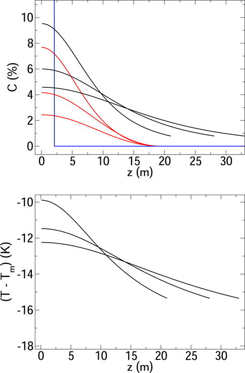
Figure 4. Top: The melted water fraction as a function of depth at different times $t=$4 months, 8 months, and 12 months. The black curves show the analytic solutions of Equation 32 in the domains where they are assumed to apply, that is, where $T<T_{\mathit{max}}$ and $M<1$. The red curves show the corresponding numerical solution of the full heat equation from Equation 32. The blue curve shows the case where there is a constant pore size and no superdiffusive spreading. Bottom: The corresponding temperature. Here, $\beta =1$, $R_{\mathit{min}}=R_{\mathit{max}}/2=$ 5 nm, and $c_b=2$MJ$/{\text{m}}^3$, as is close to both the ice and typical clay/silt values.

Figure 5

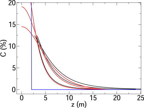
Figure 5. The same results as in Figure 4, but with $R_{\mathit{min}}=R_{\mathit{max}}/2=$ 30 nm.

Figure 6

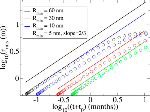
Figure 6. The increase in rms depth of the melted water fraction as a function of time for different minimum pore sizes. The time increases from $t=$ 0, and $t_0>0$ corresponds to the fact that, for numerical reasons, the initial $C(z,0)$-profile is not a $\delta$-function but has a finite width. The full lines, drawn in colors that correspond to the $(◦)$-points, show the theoretical value of Equation 48 (so, they all have slope $=2/3$) while the $(◦)$-points show the values measured from the numerical solution of Equation 32. The parameter values are the same as in Figure 4.

Even in the $R_{\mathit{min}}=$10–60 nm cases, the penetration of $C\gtrsim$ 1% fluctuations extends deeper than 10 m, as may be seen from Figure 5.

4 Discussion and conclusion

Starting from the thermodynamics of the Gibbs–Thomson effect describing the melting of ice in pores and a power law distribution of pore sizes, we have shown that the requirement of energy conservation produces a non-linear equation that yields superdiffusive spreading of the melted water fraction.

The physical picture that emerges from this analysis is that the spreading of heat, or the melted water concentration, is strongly increased by the fact that the heat will bypass any pore that is either too big for melting to occur or so small that the melting has already happened. This is true in the range of temperatures where some pores contain water and some contain ice. As a result, a subsurface porous medium containing ice will experience melting perturbations at depths that greatly exceed those that are expected from a treatment that ignores the freezing-point depression.

Formalisms involving time fractional derivatives can cover descriptions of anomalous diffusion, both in the subdiffusive and superdiffusive domains [29–31]. These formalisms are not focused on the effects of freezing-point depression as in the present case. However, they are relevant to heat flow in media with complex geometries, like porous media and fractured systems, and in some cases, they yield analytic solutions.

In the present modeling, we have neglected all effects coming from the deformations of the solid skeleton that are caused by the difference in specific volume between water and ice. While such effects are key to important phenomena like frost heave [32], they have no important role in the energy budget associated with melting and freezing that we are considering. The added work that is carried out by ice displacing parts of the solid skeleton could, in principle, be incorporated as a small correction to $\lambda$, the latent heat of fusion. This correction is ignored in the present work.

The superdiffusive spreading of temperature or melted water fraction may also be used as a method to measure pore size distributions: The estimate given in Equation 23 shows that close to $T_{\mathit{min}}$, the sensitivity to temperature variations is mainly in the pore liquid fraction $C$, and not the liquid fraction contained in the surface melted films. In the cases where the pore size distribution is in fact given by a power law distribution, the measurement of a spreading temperature profile may thus provide a value for the diffusion exponent $\tau$ and thus for the pore size distribution exponent $\beta$. Due to the higher sensitivity to the bulk pore water, this method may be superior to conventional NMR measurements, which cannot distinguish between the liquid water that resides in the pores and that which is contained in the films. Compared to mercury injection measurements, which need high pressures to probe the smallest pores, the temperature technique is less likely to alter the medium through crushing of the smallest pores. It does, however, rely on the basic assumption of a power law pore size distribution.

Our study is not restricted to pure water–solid systems. Methane hydrates, which may exist in the subsurface where glaciers have recently withdrawn, have similar values of density and latent heat as water ice [33]. This may give rise to superdíffusive behavior, even when the active substance is not water, but methane in combination with water. Measurements showing the freezing-point depression of methane and ${\text{CO}}_2$ hydrates in natural sediments [25] support this assertion.

Finally, we note that experimental verification of our predictions would be of great interest. Nanoporous man-made materials, such as activated carbons, zeolites, aluminas, mesoporous silicas, and microporous metal-organic frameworks, may all be tailored to have pores in the $\sim$ nm range. They are thus promising candidates for applications in experimental studies of superdiffusive heat flows, provided proper control and monitoring of the temperature variations are designed.

Data availability statement

The data generated by the numerical modeling can be obtained from the authors upon request.

Author contributions

EF: Writing – original draft, Methodology, Software, Conceptualization, Investigation, Formal Analysis, Funding acquisition, Writing – review and editing, Project administration. AH: Conceptualization, Funding acquisition, Writing – review and editing. EE: Conceptualization, Writing – review and editing.

Funding

The author(s) declare that financial support was received for the research and/or publication of this article. This work was partly supported by the Research Council of Norway through its Centers of Excellence funding scheme, project number 262644. AH acknowledges funding from the European Research Council (Grant Agreement 101141323 AGIPORE).

Acknowledgments

We thank Daan Frenkel for valuable suggestions on the significance of the nucleation effects.

Conflict of interest

The authors declare that the research was conducted in the absence of any commercial or financial relationships that could be construed as a potential conflict of interest.

The author(s) declared that they were an editorial board member of Frontiers, at the time of submission. This had no impact on the peer review process and the final decision.

Generative AI statement

The author(s) declare that no Generative AI was used in the creation of this manuscript.

Any alternative text (alt text) provided alongside figures in this article has been generated by Frontiers with the support of artificial intelligence and reasonable efforts have been made to ensure accuracy, including review by the authors wherever possible. If you identify any issues, please contact us.

Publisher’s note

All claims expressed in this article are solely those of the authors and do not necessarily represent those of their affiliated organizations, or those of the publisher, the editors and the reviewers. Any product that may be evaluated in this article, or claim that may be made by its manufacturer, is not guaranteed or endorsed by the publisher.

References

1. Watanabe K, Mizoguchi M. Amount of unfrozen water in frozen porous media saturated with solution. Cold regions Sci Technology (2002) 34:103–10. doi:10.1016/S0165-232X(01)00063-5

CrossRef Full Text | Google Scholar

2. Moore EB, Allen JT, Molinero V. Liquid-ice coexistence below the melting temperature for water confined in hydrophilic and hydrophobic nanopores. J Phys Chem C (2012) 116:7507–14. doi:10.1021/jp3012409

CrossRef Full Text | Google Scholar

3. Marcolli C. Deposition nucleation viewed as homogeneous or immersion freezing in pores and cavities. Atmos Chem Phys (2014) 14:2071–104. doi:10.5194/acp-14-2071-2014

CrossRef Full Text | Google Scholar

4. Campbell JM, Christenson H. Nucleation- and emergence-limited growth of ice from pores. Phys Rev Lett (2018) 120:165701. doi:10.1103/physrevlett.120.165701

PubMed Abstract | CrossRef Full Text | Google Scholar

5. Lazarenko MM, Zabashta YF, Alekseev AN, Yablochkova KS, Ushcats MV, Dinzhos RV, et al. Melting of crystallites in a solid porous matrix and the application limits of the Gibbs-Thomson equation. J Chem Phys (2022) 157:034704. doi:10.1063/5.0093327

PubMed Abstract | CrossRef Full Text | Google Scholar

6. Findenegg GH, Jähnert S, Akcakayiran D, Schreiber A. Freezing and melting of water confined in silica nanopores. ChemPhysChem (2008) 9:2651–9. doi:10.1002/cphc.200800616

PubMed Abstract | CrossRef Full Text | Google Scholar

7. Bouchaud J, Georges A. Anomalous diffusion in disordered media: statistical mechanisms, models and physical applications. Phys Rep (1990) 195:127–293. doi:10.1016/0370-1573(90)90099-n

CrossRef Full Text | Google Scholar

8. Gosh SK, Cherstvy AG, Grebenkov DS, Metzler R. Anomalous non-Gaussian tracer diffusion in crowded two-dimensional environments. New J Phys (2016) 18:013027. doi:10.1088/1367-2630/18/1/013027

CrossRef Full Text | Google Scholar

9. Richardson LF. Atmospheric diffusion shown on a distance-neighbour graph. Proc Roy Soc Lond A (1926) 110:709–37. doi:10.1098/rspa.1926.0043

CrossRef Full Text | Google Scholar

10. Schlesinger MF, West BJ, Klafter J. Levy dynamics of enhanced diffusion: application to turbulence. Phys Rev Lett (1987) 58:1100–3. doi:10.1103/PhysRevLett.58.1100

PubMed Abstract | CrossRef Full Text | Google Scholar

11. Marcolli C. Pre-activation of aerosol particles by ice preserved in pores. Atmos Chem Phys (2017) 17:1595–622. doi:10.5194/acp-17-1595-2017

CrossRef Full Text | Google Scholar

12. Hu W, Frenkel D, Mathot VBF. Free energy barrier to melting of single-chain polymer crystallite. J Chem Phys (2003) 118:3455–7. doi:10.1063/1.1553980

CrossRef Full Text | Google Scholar

13. Frenken WMJ, van der Veen JF. Observation of surface melting. Phys Rev Lett (1985) 54:134–7. doi:10.1103/physrevlett.54.134

PubMed Abstract | CrossRef Full Text | Google Scholar

14. Elbaum M, Schick M. Application of the theory of dispersion forces to the surface melting of ice. Phys Rev Lett (1991) 66:1713–6. doi:10.1103/PhysRevLett.66.1713

PubMed Abstract | CrossRef Full Text | Google Scholar

15. Wilen LA, Wettlaufer JS, Elbaum M, Schick M. Dispersion-force effects in interfacial premelting of ice. Phys Rev B (1995) 52:12426–33. doi:10.1103/physrevb.52.12426

PubMed Abstract | CrossRef Full Text | Google Scholar

16. Israelachvili JN. Intermolecular and surface forces. Elsevier (2011).

Google Scholar

17. Vehkamaki H. Classical nucleation theory in multicomponent systems. 1 edn. Berlin: Springer (2006).

Google Scholar

18. Frenkel D, Smit B. Understanding molecular simulation: from algorithms to applications. 2nd ed. Elsevier Science, Academic Press (2023).

Google Scholar

19. Daeges J, Gleiter H, Perepezko JH. Superheating of metal crystals. Phys Lett A (1986) 119:79–82. doi:10.1016/0375-9601(86)90418-4

CrossRef Full Text | Google Scholar

20. Gråbæk L, Bohr J, Anderson HH, Johansen A, Johnson E, Sarholt-Kristensen L, et al. Melting, growth and faceting of lead precipitates in aluminum. Phys Rev B (1992) 45:2628–37. doi:10.1103/physrevb.45.2628

CrossRef Full Text | Google Scholar

21. Sing K. The use of nitrogen adsorption for the characterisation of porous materials. Colloids Surf A (2001) 187:3–9. doi:10.1016/S0927-7757(01)00612-4

CrossRef Full Text | Google Scholar

22. Tombari E, Salvetti G, Ferrari C, Johari GP. Thermodynamic functions of water and ice confined to 2 nm radius pores. J Chem Phys (2005) 122:104712. doi:10.1063/1.1862244

PubMed Abstract | CrossRef Full Text | Google Scholar

23. Zhu J, Zhang R, Zhang Y, He F. The fractal characteristics of pore size distribution in cement-based materials and its effect on gas permeability. Nat Sci Rep (2019) 9:17191. doi:10.1038/s41598-019-53828-5

PubMed Abstract | CrossRef Full Text | Google Scholar

24. Zhao Y, Yu Q. CO₂ breakthrough pressure and permeability for unsaturated low-permeability sandstone of the Ordos basin. J Hydrol (2017) 550:331–42. doi:10.1016/j.jhydrol.2017.04.050

CrossRef Full Text | Google Scholar

25. Park T, Lee JY, Kwon TH. Effect of pore size distribution on dissociation temperature depression and phase boundary shift of gas hydrate in various fine-grained sediments. Energy Fuels (2018) 32:5321–30. doi:10.1021/acs.energyfuels.8b00074

CrossRef Full Text | Google Scholar

26. Crowley AB. On the weak solution of moving boundary problems. IMA J Appl Mathematics (1979) 24:43–57. doi:10.1093/imamat/24.1.43

CrossRef Full Text | Google Scholar

27. Flekkøy EG, Hansen A, Baldelli B. Hyperballistic superdiffusion and explosive solutions to the non-linear diffusion equation. Front Phys (2021) 9:41. doi:10.3389/fphy.2021.640560

CrossRef Full Text | Google Scholar

28. Pattle RE. Diffusion from an instantaneous point source with a concentration-dependent coefficient. Mech Appl Math (1959) 12:407–9. doi:10.1093/qjmam/12.4.407

CrossRef Full Text | Google Scholar

29. Žecová M, Terpák J. Heat conduction modeling by using fractional-order derivatives. Appl Math Comput (2015) 257:365–73. doi:10.1016/j.amc.2014.12.136

CrossRef Full Text | Google Scholar

30. Suzuki A, Fomin SA, Chugunov VA, Niibori Y, Hashida T. Fractional diffusion modeling of heat transfer in porous and fractured media. Int J Heat Mass Transfer (2016) 103:611–8. doi:10.1016/j.ijheatmasstransfer.2016.08.002

CrossRef Full Text | Google Scholar

31. Nikan O, Avazzadeh Z, Machado JT. Numerical approach for modeling fractional heat conduction in porous medium with the generalized Cattaneo model. Appl Math Model (2021) 100:107–24. doi:10.1016/j.apm.2021.07.025

CrossRef Full Text | Google Scholar

32. Rempel AW, Wettlaufer JS, Worster MG. Premelting dynamics in a continuum model of frost heave. J Fluid Mech (2004) 498:227–44. doi:10.1017/s0022112003006761

CrossRef Full Text | Google Scholar

33. Chuvilin E, Davletshina D. Formation and accumulation of pore methane hydrates in permafrost: experimental modeling. Geosciences (2018) 8:467. doi:10.3390/geosciences8120467

CrossRef Full Text | Google Scholar