Treatment of a generalized scalar differential epquation: analysis and explicit solution

Obtaining a solution of a given SDE is essential in neuroscience, especially, in modeling transmission of nerve impulses between neurons through myelin substance. This paper analyzes a particular scalar differential equation (SDE). The current scalar model involves two categories of differential equations–advanced and delayed–based on the domain of the independent variable. The results are consistent with existing literature as the advance/delay parameter approaches unity. Theoretical and graphical analyses of the solution’s properties are presented. To the best of our knowledge, this is the first study to analyze this form of SDE.

1 Introduction

In ordinary differential equations (ODEs), the equation $y^{\prime }(t)=\alpha y(t)+\beta y(t-\tau )$ is typically classified as a delay differential equation (DDE) in the domain $t>0$, since $t-\tau <t$ for any $\tau >0$, with $\tau$ serving as the delay parameter. Conversely, the equation $y^{\prime }(t)=\alpha y(t)+\beta y(t+\tau )$ is considered an advanced differential equation (ADE) in the domain $t>0$, as $t+\tau >t$ for all $t,\tau >0$, with $\tau$ interpreted as the advance parameter. However, if an ODE involves both delay and advance terms in distinct but connected domains, it is more appropriately classified as a scalar differential equation (SDE). In the examples above, the terms $y(t-\tau )$ and $y(t+\tau )$ involve positive coefficients of the independent variable $t$, allowing straightforward classification of the respective equations as DDE and ADE.

A question arises here: what is the type of the second ODE if $y(t+\tau )$ is changed to $y(-t+\tau )$? Answering this question requires two steps to determine the domains of $t$ for which $-t+\tau <t$ (delay) and $-t+\tau >t$ (advance). The first step, $-t+\tau <t$ implies $t>\tau /2$, while the second step, $-t+\tau >t$ leads to $t<\tau /2$. Based on this, the ODE $y^{\prime }(t)=\alpha y(t)+\beta y(-t+\tau )$ can be classified as an ADE in the domain $0<t<\tau /2$, and as a DDE in the domain $\tau /2<t<\infty$. Hence, we may refer to the ODE $y^{\prime }(t)=\alpha y(t)+\beta y(-t+\tau )$ as an SDE because it involves both types of advance and delay equations, as pointed out in Refs. [1, 2]. Another important observation concerns the central point connecting the two domains, which is $t=\tau /2$. This central point plays a fundamental role in deriving the analytical solutions of a given SDE, as will be demonstrated later. It is also useful to distinguish between proportional delay parameters and pure delay parameters. In the DDE $y^{\prime }(t)=\alpha y(t)+\beta y(t-\tau )$, the parameter $\tau$ is referred to as a pure delay parameter. However, other types of DDEs involve proportional delay parameters, such as in the pantograph equation (PE) $y^{\prime }(t)=\alpha y(t)+\beta y(\gamma t)$, $0<\gamma <1$ [3, 4]. The PE has applications in modeling the behavior of overhead catenary systems for railway electrification [5–7], the dynamic response of trolley wire overhead contact systems for electric railways [8], and current collection systems in electric locomotives [9]. Several authors have analyzed the PE in detail [10–12]. Another notable example is the Ambartsumian equation (AE), given by $y^{\prime }(t)=-y(t)+\frac{1}{q}y\left(\frac{t}{q}\right)$, where $q>1$. This equation has practical significance in astronomy, particularly in studies of surface brightness in the Milky Way [13–16]. In these models, $\gamma$ and $1/q$ are considered proportional delay parameters. For the pantograph model, $0<\gamma <1$ implies $\gamma t<t$ indicating a delay for all $t>0$. Similarly, the Ambartsumian model $\frac{t}{q}<t$ also represents a delay.

In this paper, we consider the following general form of the SDE:

$y^{\prime }\left(t\right)=\alpha y\left(t\right)+\beta y\left(-ct+\tau \right),y\left(t\right)=0\forall t<0,y\left(0\right)=\lambda ,0<c\le 1,\tau >0,(1)$

where $\alpha$, $\beta$, and $\lambda$ are real constants. It can be readily shown that Equation 1 represents an advanced equation in the domain $0<t<\frac{\tau }{c+1}$, while it becomes a delayed equation for $t>\frac{\tau }{c+1}$. Finding a solution to Equation 1 poses a significant challenge and, to the best of our knowledge, may be considered for the first time. Moreover, standard methods such as the Adomian decomposition method (ADM) [17–20], the homotopy perturbation method [21, 22], and the Laplace transform (LT) [23–26] may encounter difficulties when applied to such problems.

To address this, a direct series approach is developed to solve the advanced equation. A closed-form expression of the series is obtained, and its convergence is established theoretically. These results are then used to construct the solution for the delayed equation. Several existing results in the literature can be recovered as special cases of the present findings. In addition, the properties of the obtained solutions are analyzed both theoretically and graphically. Finding a solution for a SDE is helpful for understanding the transmission of nerve impulses between neurons through myelin substance which covers all the nerves in the brain and nervous system in humans [27]. Other areas of applications can be further extended to involve some recent dynamical systems [28–30] and relatively new physical phenomena [31, 32].

2 Advanced equation $0<t<\frac{\tau }{c+1}$

In the domain $0<t<\frac{\tau }{c+1}$, SDE (1) becomes an advanced equation since $-ct+\tau >t\forall t\in \left(0,\frac{\tau }{c+1}\right)$, $0<c\le 1$. Moreover, in the advanced equation domain, $\frac{\tau }{c+1}<-ct+\tau <\tau$, see Refs. [1, 2] for details. Accordingly, the value of the function $y\left(-ct+\tau \right)$ is unknown, which prevents the application of the step method to solve the advanced equation:

$y^{\prime }\left(t\right)=\alpha y\left(t\right)+\beta y\left(-ct+\tau \right),y\left(t\right)=0\forall t<0,y\left(0\right)=\lambda ,0<c\le 1,\tau >0,0<t<\frac{\tau }{c+1}.(2)$

Before discussing the main objective of this section, it is important to note that the condition:

$y^{\prime }\left(\frac{\tau }{c+1}\right)=\left(\alpha +\beta \right)y\left(\frac{\tau }{c+1}\right),(3)$

must be satisfied by any solution to Equation 2 in addition to the initial condition (IC) $y(0)=\lambda$.

2.1 Closed-form series solution

An effective solution for a given model can be derived as a closed-form series solution. The solution in such a form facilitates numerical calculations and also leads to easier analysis to study the properties/behavior of the physical system. Let us attempt a series of solutions in the form of:

$y\left(t\right)={\displaystyle \sum _{n=0}^{\infty }}{a}_n{\left(t-\frac{\tau }{c+1}\right)}^n.(4)$

This assumption yields:

$y^{\prime }\left(t\right)={\displaystyle \sum _{n=0}^{\infty }}\left(n+1\right)a_{n+1}{\left(t-\frac{\tau }{c+1}\right)}^n,(5)$

and

$y\left(-ct+\tau \right)={\displaystyle \sum _{n=0}^{\infty }}{\left(-c\right)}^n{a}_n{\left(t-\frac{\tau }{c+1}\right)}^n.(6)$

Substituting Equations 4–6 into Equation 2 leads to:

$a_{n+1}=\frac{a_n}{n+1}\left(\alpha +{\left(-c\right)}^n\beta \right),n\ge 0.(7)$

Hence,

$a_{n+1}=\frac{a_0}{\left(n+1\right)!}\prod _{k=0}^n\left(\alpha +{\left(-c\right)}^k\beta \right),n\ge 0.(8)$

From (4), we can write:

$y\left(t\right)=a_0+{\displaystyle \sum _{n=0}^{\infty }}{a}_{n+1}{\left(t-\frac{\tau }{c+1}\right)}^{n+1}.(9)$

Employing (8), we obtain:

$y\left(t\right)=a_0\left[1+{\displaystyle \sum _{n=0}^{\infty }}\frac{1}{\left(n+1\right)!}\prod _{k=0}^n\left(\alpha +{\left(-c\right)}^k\beta \right){\left(t-\frac{\tau }{c+1}\right)}^{n+1}\right],(10)$

or

$y\left(t\right)=a_0\left[1+{\displaystyle \sum _{n=0}^{\infty }}{h}_n{\left(t-\frac{\tau }{c+1}\right)}^{n+1}\right],(11)$

where

$h_n=\frac{1}{\left(n+1\right)!}\prod _{k=0}^n\left(\alpha +{\left(-c\right)}^k\beta \right),n\ge 0.(12)$

By applying IC $y(0)=\lambda$ to Equation 11, we get:

$a_0=\frac{\lambda }{1+{\sum }_{n=0}^{\infty }{h}_n{\left(-\frac{\tau }{c+1}\right)}^{n+1}}.(13)$

Substituting (13) into (11) yields:

$y\left(t\right)=\lambda \left[\frac{1+{\sum }_{n=0}^{\infty }{h}_n{\left(t-\frac{\tau }{c+1}\right)}^{n+1}}{1+{\sum }_{n=0}^{\infty }{h}_n{\left(-\frac{\tau }{c+1}\right)}^{n+1}}\right].(14)$

Equation 14 declares that IC $y(0)=\lambda$ is satisfied automatically. Let us now check the satisfaction of condition (3). For this purpose, from the solution (14), we obtain:

$y\left(\frac{\tau }{c+1}\right)=\frac{\lambda }{1+{\sum }_{n=0}^{\infty }{h}_n{\left(-\frac{\tau }{c+1}\right)}^{n+1}}=a_0,(15)$

and

$y^{\prime }\left(\frac{\tau }{c+1}\right)=\frac{\lambda h_0}{1+{\sum }_{n=0}^{\infty }{h}_n{\left(-\frac{\tau }{c+1}\right)}^{n+1}}=\left(\alpha +\beta \right)a_0,(16)$

where Equation 12 is implemented to calculate $h_0=\alpha +\beta$. The last two equations show that condition (3) is also satisfied. The next step is to examine the convergence of the obtained series solution, which is discussed in the following subsection.

2.2 Convergence analysis

To provide a theoretical proof of the convergence of the series solution (14), it is sufficient to prove the convergence of the series ${\sum }_{n=0}^{\infty }{h}_n{\left(t-\frac{\tau }{c+1}\right)}^{n+1}$ in the domain $0<t<\frac{\tau }{c+1}$.

Theorem 1. For $0<c\le 1$, the series:

${\displaystyle \sum _{n=0}^{\infty }}{h}_n{\left(t-\frac{\tau }{c+1}\right)}^{n+1},(17)$

converge in the domain $0<t<\frac{\tau }{c+1}$.

Proof.Let us define,

${\rho }_n\left(t\right)=h_n{\left(t-\frac{\tau }{c+1}\right)}^{n+1}.(18)$

Applying the ratio test:

$\underset{n\to \infty }{\lim }\left|\frac{{\rho }_{n+1}\left(t\right)}{{\rho }_n\left(t\right)}\right|=\underset{n\to \infty }{\lim }\left|\frac{h_{n+1}}{h_n}\left(t-\frac{\tau }{c+1}\right)\right|.(19)$

Hence,

$\underset{n\to \infty }{\lim }\left|\frac{{\rho }_{n+1}\left(t\right)}{{\rho }_n\left(t\right)}\right|=\left|t-\frac{\tau }{c+1}\right|\underset{n\to \infty }{\lim }\left|\frac{\alpha +{\left(-c\right)}^{n+1}\beta }{n+2}\right|.(20)$

The limit on the right-hand side of the last equation tends toward zero as $n\to \infty$ for every $0<c<1$ and $0<t<\frac{\tau }{c+1}$. At $c=1$, the value ${(-c)}^{n+1}=\pm 1$ according to $n$. In this case, Equation 20 becomes:

$\underset{n\to \infty }{\lim }\left|\frac{{\rho }_{n+1}\left(t\right)}{{\rho }_n\left(t\right)}\right|=\left|t-\frac{\tau }{c+1}\right|\underset{n\to \infty }{\lim }\left|\frac{\alpha \pm \beta }{n+2}\right|,(21)$

which also tends toward zero, thereby completing the proof.

Remark 1. Through a similar analysis, we can easily prove that the series ${\sum }_{n=0}^{\infty }{h}_n{\left(-\frac{\tau }{c+1}\right)}^{n+1}$ is convergent for all $c\in (\mathrm{0,1}]$.

2.3 Special case and exact solution

In this section, we show that the obtained series solution in Section 2.1 converges to the exact hyperbolic and trigonometric forms when $c=1$ under the conditions $\alpha >\beta$ and $\beta >\alpha$, respectively. We consider $c=1$ in Equation 2 and then extract the solution of the corresponding advanced equation:

$y^{\prime }\left(t\right)=\alpha y\left(t\right)+\beta y\left(-t+\tau \right),y\left(t\right)=0\forall t<0,y\left(0\right)=\lambda ,\tau >0,0<t<\frac{\tau }{2}.(22)$

In this case, the solution given by Equation 14 reads:

$y\left(t\right)=\lambda \left[\frac{1+{\sum }_{n=0}^{\infty }{h}_n{\left(t-\frac{\tau }{2}\right)}^{n+1}}{1+{\sum }_{n=0}^{\infty }{h}_n{\left(-\frac{\tau }{2}\right)}^{n+1}}\right],(23)$

where $h_n$ in Equation 12 becomes:

$h_n=\frac{1}{\left(n+1\right)!}\prod _{k=0}^n\left(\alpha +{\left(-1\right)}^k\beta \right),n\ge 0.(24)$

This equation can be used to generate the following equations for the even-order coefficients $h_{2n}$ and odd-order coefficients $h_{2n+1}$ as follows:

$h_{2n}=\frac{{\omega }^{2n}}{\left(2n+1\right)!}\left(\alpha +\beta \right),h_{2n+1}=\frac{{\omega }^{2n+2}}{\left(2n+2\right)!},\omega =\sqrt{{\alpha }^2-{\beta }^2},\alpha >\beta ,n\ge 0.(25)$

The numerator of solution (23) can be written as follows:

$\begin{array}{cc}\hfill 1+{\displaystyle \sum _{n=0}^{\infty }}{h}_n{\left(t-\frac{\tau }{2}\right)}^{n+1}& =1+{\displaystyle \sum _{n=0}^{\infty }}{h}_{2n}{\left(t-\frac{\tau }{2}\right)}^{2n+1}+{\displaystyle \sum _{n=0}^{\infty }}{h}_{2n+1}{\left(t-\frac{\tau }{2}\right)}^{2n+2},\hfill \\ \hfill & =1+\frac{\alpha +\beta }{\omega }{\displaystyle \sum _{n=0}^{\infty }}\frac{{\left(\omega \left(t-\frac{\tau }{2}\right)\right)}^{2n+1}}{\left(2n+1\right)!}+{\displaystyle \sum _{n=0}^{\infty }}\frac{{\left(\omega \left(t-\frac{\tau }{2}\right)\right)}^{2n+2}}{\left(2n+2\right)!},\hfill \\ \hfill & =\frac{\alpha +\beta }{\omega }\sinh \left[\omega \left(t-\frac{\tau }{2}\right)\right]+\cosh \left[\omega \left(t-\frac{\tau }{2}\right)\right].\hfill \end{array}(26)$

Similarly, the denominator of solution (23) can be written as follows:

$1+{\displaystyle \sum _{n=0}^{\infty }}{h}_n{\left(-\frac{\tau }{2}\right)}^{n+1}=\cosh \left(\frac{\omega \tau }{2}\right)-\frac{\alpha +\beta }{\omega }\sinh \left(\frac{\omega \tau }{2}\right).(27)$

Substituting (26) and (27) into (23), we obtain the exact hyperbolic solution:

$y\left(t\right)=\lambda \left[\frac{\omega \cosh \left[\omega \left(t-\frac{\tau }{2}\right)\right]+\left(\alpha +\beta \right)\sinh \left[\omega \left(t-\frac{\tau }{2}\right)\right]}{\omega \cosh \left(\frac{\omega \tau }{2}\right)-\left(\alpha +\beta \right)\sinh \left(\frac{\omega \tau }{2}\right)}\right].(28)$

Moreover, if we rewrite the coefficients $h_{2n}$ and $h_{2n+1}$ as follows:

$\begin{array}{ll}\hfill h_{2n}& =\frac{{\left(-1\right)}^n{\mathrm{\Omega }}^{2n}}{\left(2n+1\right)!}\left(\alpha +\beta \right),h_{2n+1}=\frac{{\left(-1\right)}^{n+1}{\mathrm{\Omega }}^{2n+2}}{\left(2n+2\right)!},\hfill \\ \hfill & \mathrm{\Omega }=\sqrt{{\beta }^2-{\alpha }^2},\beta >\alpha ,n\ge 0,\hfill \end{array}(29)$

then, we can arrive at the exact periodic solution:

$y\left(t\right)=\lambda \left[\frac{\mathrm{\Omega }\cos \left[\omega \left(t-\frac{\tau }{2}\right)\right]+\left(\alpha +\beta \right)\sin \left[\mathrm{\Omega }\left(t-\frac{\tau }{2}\right)\right]}{\mathrm{\Omega }\cos \left(\frac{\mathrm{\Omega }\tau }{2}\right)-\left(\alpha +\beta \right)\sin \left(\frac{\mathrm{\Omega }\tau }{2}\right)}\right].(30)$

Solution (30) agrees with the corresponding values obtained in Ref. [1] for the advanced Equation 22.

3 Delay equation $t>\frac{\tau }{c+1}$

It may be useful to divide the domain $t>\frac{\tau }{c+1}$ into two intervals, $\frac{\tau }{c+1}<t<\frac{\tau }{c}$ and $t>\frac{\tau }{c}$. This is simply because the value of $y(-ct+\tau )$ in each of the above two intervals can be assigned a certain value, as described in the next subsections. To achieve our target, we first denote $y_1(t)$ as the solution in the interval $0<t<\frac{\tau }{c+1}$; hence,

$y\left(t\right)=y_1\left(t\right)=a_0\left[1+{\displaystyle \sum _{n=0}^{\infty }}{h}_n{\left(t-\frac{\tau }{c+1}\right)}^{n+1}\right],0<t<\frac{\tau }{c+1},(31)$

where $a_0$ is given by Equation 11.

3.1 Solution in interval $\frac{\tau }{c+1}<t<\frac{\tau }{c}$

In the interval $\frac{\tau }{c+1}<t<\frac{\tau }{c}$ we find that $0<-ct+\tau <\frac{\tau }{c+1}$ and accordingly Equation 31 gives:

$y\left(-ct+\tau \right)=y_1\left(-ct+\tau \right)=a_0\left[1+{\displaystyle \sum _{n=0}^{\infty }}{\left(-c\right)}^{n+1}{h}_n{\left(t-\frac{\tau }{c+1}\right)}^{n+1}\right].(32)$

The advanced equation in this interval takes the form:

$y^{\prime }\left(t\right)=\alpha y\left(t\right)+\beta y_1\left(-ct+\tau \right),y\left(t\right)=y_1\left(t\right)\forall t\in \left(0,\frac{\tau }{c+1}\right),\frac{\tau }{c+1}<t<\frac{\tau }{c},(33)$

subject to

$y\left(\frac{\tau }{c+1}\right)=y_1\left(\frac{\tau }{c+1}\right)=a_0.(34)$

Substituting (32) into (33) results in the following ODE:

$y^{\prime }\left(t\right)-\alpha y\left(t\right)=\beta a_0\left[1+{\displaystyle \sum _{n=0}^{\infty }}{\left(-c\right)}^{n+1}{h}_n{\left(t-\frac{\tau }{c+1}\right)}^{n+1}\right],\frac{\tau }{c+1}<t<\frac{\tau }{c}.(35)$

Solving this ODE under Condition (34) yields

$y\left(t\right)=a_0{e}^{\alpha \left(t-\frac{\tau }{c+1}\right)}+\frac{a_0\beta }{\alpha }\left[e^{\alpha \left(t-\frac{\tau }{c+1}\right)}-1\right]+a_0\beta e^{\alpha t}{\displaystyle \sum _{n=0}^{\infty }}{\left(-c\right)}^{n+1}{h}_n{I}_n\left(t\right),(36)$

where

$I_n\left(t\right)={\int }_{\frac{\tau }{c+1}}^t{e}^{-\alpha t}{\left(t-\frac{\tau }{c+1}\right)}^{n+1}dt.(37)$

This integral appears complex; however, it can be evaluated analytically in terms of the generalized incomplete gamma function $\mathrm{\Gamma }(m,z_1,z_2)$ defined by:

$\mathrm{\Gamma }\left(m,z_1,z_2\right)={\int }_{z_1}^{z_2}{e}^{-t}{t}^{m-1}dt.(38)$

The integral (37) can be determined by:

$I_n\left(t\right)={\alpha }^{-\left(n+2\right)}{e}^{-\frac{\alpha \tau }{c+1}}\mathrm{\Gamma }\left(n+\mathrm{2,0},\alpha \left(t-\frac{\tau }{c+1}\right)\right).(39)$

Therefore, the solution (36) takes the following form:

$\begin{array}{ll}\hfill y\left(t\right)& =-\frac{a_0\beta }{\alpha }+e^{\alpha \left(t-\frac{\tau }{c+1}\right)}\left[a_0\left(1+\frac{\beta }{\alpha }\right)-\frac{a_0\beta }{\alpha }{\displaystyle \sum _{n=0}^{\infty }}{\left(-\frac{c}{\alpha }\right)}^{n+1}\right.\hfill \\ \hfill & \left.h_n\mathrm{\Gamma }\left(n+\mathrm{2,0},\alpha \left(t-\frac{\tau }{c+1}\right)\right)\right].\hfill \end{array}(40)$

The series on the right-hand side of this equation must also be checked for convergence, which is discussed in the next theorem.

Theorem 2. For $0<c\le 1$, the series

${\displaystyle \sum _{n=0}^{\infty }}{\left(-\frac{c}{\alpha }\right)}^{n+1}{h}_n\mathrm{\Gamma }\left(n+\mathrm{2,0},\alpha \left(t-\frac{\tau }{c+1}\right)\right),(41)$

converges in the domain $\frac{\tau }{c+1}<t<\frac{\tau }{c}$.

Proof.Assume that,

${\sigma }_n\left(t\right)=h_n{\left(t-\frac{\tau }{c+1}\right)}^{n+1}.(42)$

Applying the ratio test:

$\underset{n\to \infty }{\lim }\left|\frac{{\sigma }_{n+1}\left(t\right)}{{\sigma }_n\left(t\right)}\right|=\underset{n\to \infty }{\lim }\left|-\frac{c}{\alpha }\frac{h_{n+1}}{h_n}\frac{\mathrm{\Gamma }\left(n+\mathrm{3,0},\alpha \left(t-\frac{\tau }{c+1}\right)\right)}{\mathrm{\Gamma }\left(n+\mathrm{2,0},\alpha \left(t-\frac{\tau }{c+1}\right)\right)}\right|,(43)$

i.e.,

$\underset{n\to \infty }{\lim }\left|\frac{{\rho }_{n+1}\left(t\right)}{{\rho }_n\left(t\right)}\right|=\left|\frac{c}{\alpha }\right|\underset{n\to \infty }{\lim }\left|\frac{h_{n+1}}{h_n}\right|\times \underset{n\to \infty }{\lim }\left|\frac{\mathrm{\Gamma }\left(n+\mathrm{3,0},\alpha \left(t-\frac{\tau }{c+1}\right)\right)}{\mathrm{\Gamma }\left(n+\mathrm{2,0},\alpha \left(t-\frac{\tau }{c+1}\right)\right)}\right|.(44)$

We obtain:

$\underset{n\to \infty }{\lim }\left|\frac{\mathrm{\Gamma }\left(n+\mathrm{3,0},\alpha \left(t-\frac{\tau }{c+1}\right)\right)}{\mathrm{\Gamma }\left(n+\mathrm{2,0},\alpha \left(t-\frac{\tau }{c+1}\right)\right)}\right|=\alpha \left(t-\frac{\tau }{c+1}\right).(45)$

Therefore,

$\underset{n\to \infty }{\lim }\left|\frac{{\rho }_{n+1}\left(t\right)}{{\rho }_n\left(t\right)}\right|=c\left|t-\frac{\tau }{c+1}\right|\underset{n\to \infty }{\lim }\left|\frac{\alpha +{\left(-c\right)}^{n+1}\beta }{n+2}\right|.(46)$

The limit on the right-hand side tends to zero as $n\to \infty$ for every $0<c\le 1$, thus completing the proof.

3.2 Solution in interval $t>\frac{\tau }{c}$

Let us define $y(t)=y_2(t)$ as the solution in the previous interval $\frac{\tau }{c+1}<t<\frac{\tau }{c}$. At $t=\frac{\tau }{c}$, we get $y\left(\frac{\tau }{c}\right)=y_2\left(\frac{\tau }{c}\right)=\delta$, where

$\begin{array}{ll}\hfill \delta & =-\frac{a_0\beta }{\alpha }+e^{\frac{\alpha \tau }{c\left(c+1\right)}}\left[a_{0}no\left(1+\frac{\beta }{\alpha }\right)n-e\frac{a_0\beta }{\alpha }e{\displaystyle \sum _{n=0}^{\infty }}e{\left(-\frac{c}{\alpha }\right)}^{n+1}\right.\hfill \\ \hfill & \left.n{h}_{n}on\mathrm{\Gamma }\left(n+\mathrm{2,0},\frac{\alpha \tau }{c\left(c+1\right)}\right)\right].\hfill \end{array}(47)$

In the interval $t>\tau /c$, we have $-ct+\tau <0$ which yields $y(-ct+\tau )=0$. Therefore, the delay equation is reduced to:

$y^{\prime }\left(t\right)-\alpha y\left(t\right)=0,y\left(t\right)=y_2\left(t\right)\forall t\in \left(\frac{\tau }{c+1},\frac{\tau }{c}\right),t>\frac{\tau }{c}.(48)$

The solution to this ODE is as follows:

$y\left(t\right)=\delta e^{\alpha \left(t-\frac{\tau }{c}\right)},t>\frac{\tau }{c}.(49)$

4 Results

The objective of this section is to extract the numerical results for the convergence of the obtained series solutions for the advanced equation in the interval $0<t<\frac{\tau }{c+1}$ and for the delay equation in the intervals $\frac{\tau }{c+1}<t<\frac{\tau }{c}$ and $t>\frac{\tau }{c}$. Since the obtained solutions are expressed in terms of an infinite series, which was proven theoretically for convergence, one may replace infinity with a finite number. Let us denote ${\varphi }_m(t)$, ${\psi }_m(t)$, and ${\chi }_m(t)$ as the $m$-term approximate solutions for the obtained solutions in the intervals $0<t<\frac{\tau }{c+1}$, $\frac{\tau }{c+1}<t<\frac{\tau }{c}$, and $t>\frac{\tau }{c}$, respectively. Accordingly, we obtain:

${\varphi }_m\left(t\right)=a_0\left[1+{\displaystyle \sum _{n=0}^{m-1}}{h}_n{\left(t-\frac{\tau }{c+1}\right)}^{n+1}\right],a_0=\lambda /\left(1+{\displaystyle \sum _{n=0}^{m-1}}{h}_n{\left(-\frac{\tau }{c+1}\right)}^{n+1}\right),(50)$

and

$\begin{array}{ll}\hfill {\psi }_m\left(t\right)& =-\frac{a_0\beta }{\alpha }+e^{\alpha \left(t-\frac{\tau }{c+1}\right)}\left[a_0\left(1+\frac{\beta }{\alpha }\right)-\frac{a_0\beta }{\alpha }{\displaystyle \sum _{n=0}^{m-1}}{\left(-\frac{c}{\alpha }\right)}^{n+1}\right.\hfill \\ \hfill & \left.h_n\mathrm{\Gamma }\left(n+\mathrm{2,0},\alpha \left(t-\frac{\tau }{c+1}\right)\right)\right],\hfill \end{array}(51)$

while ${\chi }_m(t)$ can be written as follows:

$\begin{array}{ll}\hfill {\chi }_m\left(t\right)& =e^{\alpha \left(t-\frac{\tau }{c}\right)}/\left(-\frac{a_0\beta }{\alpha }+e^{\frac{\alpha \tau }{c\left(c+1\right)}}\left[a_0\left(1+\frac{\beta }{\alpha }\right)\right.\right.\hfill \\ \hfill & \left.\left.-\frac{a_0\beta }{\alpha }{\displaystyle \sum _{n=0}^{m-1}}{\left(-\frac{c}{\alpha }\right)}^{n+1}{h}_n\mathrm{\Gamma }\left(n+\mathrm{2,0},\frac{\alpha \tau }{c\left(c+1\right)}\right)\right]\right).\hfill \end{array}(52)$

Figures 1–3 show the curves of the approximations ${\varphi }_m(t)$, ${\psi }_m(t)$, and ${\chi }_m(t)$ at $m=\mathrm{2,3,4,5}$ when $\lambda =1$, $\alpha =-1$, $\beta =3$, $c=1/2$, and $\tau =3$. It can be seen in these figures that the convergence of the solutions in the above three intervals is achieved using few terms. The same conclusion applies to the curves shown in Figures 4–6 when $\lambda =1$, $\alpha =-5$, $\beta =-2$, $c=1/2$, and $\tau =3/2$.

Figure 1

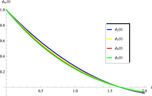
Figure 1. Convergence of approximations ${\varphi }_m(t)$ for advanced equation in interval $(0,\tau /(c+1))$ at $m=\mathrm{2,3,4,5}$ when $\lambda =1$, $\alpha =-1$, $\beta =3$, $c=1/2$, and $\tau =3$.

Figure 2

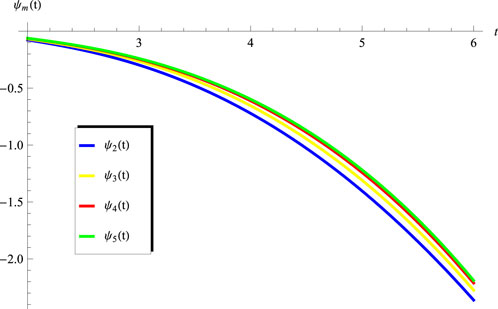
Figure 2. Convergence of approximations ${\psi }_m(t)$ for delay equation in interval $(\tau /(c+1),\tau /c)$ at $m=\mathrm{2,3,4,5}$ when $\lambda =1$, $\alpha =-1$, $\beta =3$, $c=1/2$, and $\tau =3$.

Figure 3

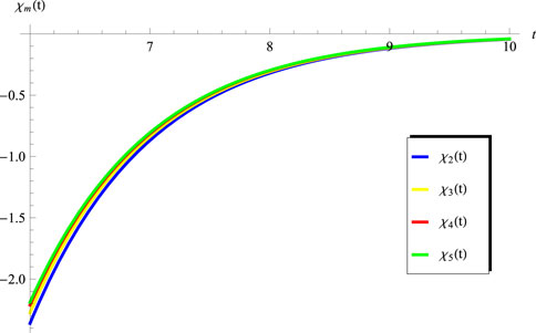
Figure 3. Convergence of approximations ${\chi }_m(t)$ for delay equation in interval $(\tau /c,\infty )$ at $m=\mathrm{2,3,4,5}$ when $\lambda =1$, $\alpha =-1$, $\beta =3$, $c=1/2$, and $\tau =3$.

Figure 4

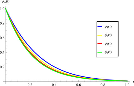
Figure 4. Convergence of approximations ${\varphi }_m(t)$ for advanced equation in interval $(0,\tau /(c+1))$ at $m=\mathrm{5,6,7,8}$ when $\lambda =1$, $\alpha =-5$, $\beta =-2$, $c=1/2$, and $\tau =3/2$.

Figure 5

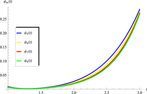
Figure 5. Convergence of approximations ${\psi }_m(t)$ for delay equation in interval $(\tau /(c+1),\tau /c)$ at $m=\mathrm{5,6,7,8}$ when $\lambda =1$, $\alpha =-5$, $\beta =-2$, $c=1/2$, and $\tau =3/2$.

Figure 6

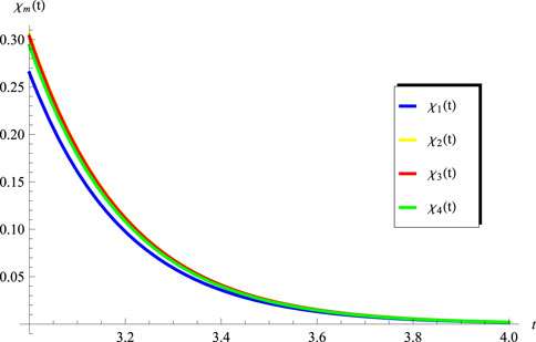
Figure 6. Convergence of approximations ${\chi }_m(t)$ for delay equation in interval $(\tau /c,\infty )$ at $m=\mathrm{1,2,3,4}$ when $\lambda =1$, $\alpha =-5$, $\beta =-2$, $c=1/2$, and $\tau =3/2$.

The behavior of the solution in the full domain is depicted in Figures 7, 8 for the same set of values of the constants used to generate Figures 1, 4, respectively. It should be noted that the solutions plotted in Figures 7, 8 are produced using the terms in series (50)–(52).

Figure 7

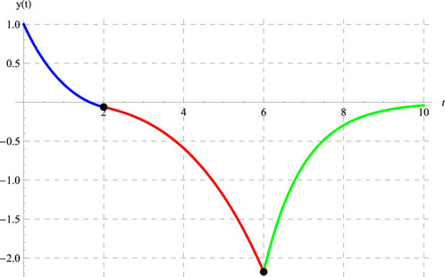
Figure 7. Plot of $y(t)$ at $\lambda =1$, $\alpha =-1$, $\beta =3$, and $c=1/2$ when $\tau =3$.

Figure 8

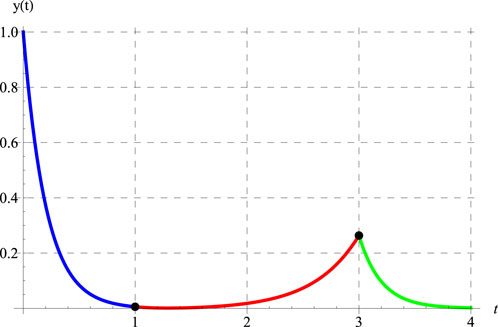
Figure 8. Plot of $y(t)$ at $\lambda =1$, $\alpha =-5$, $\beta =-2$, and $c=1/2$ when $\tau =3/2$.

The two black dots shown in Figures 7, 8 represent the three intervals $0<t<\frac{\tau }{c+1}$, $\frac{\tau }{c+1}<t<\frac{\tau }{c}$ and $t>\frac{\tau }{c}$. In addition, these dots represent the approximate values of $y_1\left(\frac{\tau }{c+1}\right)\approx {\varphi }_{10}\left(\frac{\tau }{c+1}\right)$ and $y_2\left(\frac{\tau }{c}\right)\approx {\psi }_{10}\left(\frac{\tau }{c}\right)$. However, Figures 7, 8 indicate that the solution is continuous at the joint points, where ${\varphi }_{10}\left(\frac{\tau }{c+1}\right)={\psi }_{10}\left(\frac{\tau }{c+1}\right)$ and ${\psi }_{10}\left(\frac{\tau }{c}\right)={\chi }_{10}\left(\frac{\tau }{c}\right)$.

Regarding the continuity of the derivative $y^{\prime }(t)$, we can prove that $y^{\prime }(t)$ is continuous at $t=\frac{\tau }{c+1}$ but discontinuous at $t=\frac{\tau }{c}$.

This conclusion can be explained theoretically as follows. At $t=\frac{\tau }{c+1}$, we obtain Equation 2. The left derivative is $y_1^{\prime }\left(\frac{\tau }{c+1}\right)=(\alpha +\beta )y_1\left(\frac{\tau }{c+1}\right)$, and the right derivative is derived from Equation 33 as $y_2^{\prime }\left(\frac{\tau }{c+1}\right)=(\alpha +\beta )y_2\left(\frac{\tau }{c+1}\right)$. Since $y_1\left(\frac{\tau }{c+1}\right)=y_2\left(\frac{\tau }{c+1}\right)$, then $y_1^{\prime }\left(\frac{\tau }{c+1}\right)=y_2^{\prime }\left(\frac{\tau }{c+1}\right)$; hence, $y^{\prime }(t)$ is always continuous at $t=\frac{\tau }{c+1}$.

At $t=\frac{\tau }{c}$, Equation 33 gives the left derivative as $y_2^{\prime }\left(\frac{\tau }{c}\right)=\alpha y_2\left(\frac{\tau }{c}\right)+\beta y_1(0)$, i.e., $y_2^{\prime }\left(\frac{\tau }{c}\right)=\alpha y_2\left(\frac{\tau }{c}\right)+\beta \lambda$. Equation 48 yields the right derivative at $t=\frac{\tau }{c}$ as $y_3^{\prime }\left(\frac{\tau }{c}\right)=\alpha y_3\left(\frac{\tau }{c}\right)$.

Since $y_2\left(\frac{\tau }{c}\right)=y_3\left(\frac{\tau }{c}\right)$, then $y_2^{\prime }\left(\frac{\tau }{c}\right)-y_3^{\prime }\left(\frac{\tau }{c}\right)=\beta \lambda$, which leads to $y_2^{\prime }\left(\frac{\tau }{c}\right)\ne y_3^{\prime }\left(\frac{\tau }{c}\right)$, where $\lambda \ne 0$ and $\beta \ne 0$ are assumed.

5 Conclusion

A new type of differential equation was addressed and solved in this study. The model took the form of SDE, $y^{\prime }(t)=\alpha y(t)+\beta y\left(-ct+\tau \right)$, where $0<c\le 1$ and $\tau >0$. The SDE splits into an advanced equation and delay equation in the domains $0<t<\tau /(c+1)$ and $t>\tau /(c+1)$, respectively. The solution of the advanced equation was obtained in a closed series form, for which convergence was theoretically proven. As $c$ tended toward unity, the series solution for the advanced equation transformed into exact hyperbolic and trigonometric forms for $\alpha >\beta$ and $\beta >\alpha$, respectively. The solution of the delay equation was explicitly determined in terms of the incomplete gamma function using a stepwise method. The results agreed with those in the literature when $c$ tended toward unity. The properties of the solutions were analyzed both theoretically and graphically. The results showed that the solution $y(t)$ was continuous over the full domain of the problem. Additionally, the derivative $y^{\prime }(t)$ remained continuous at the point $t=\tau /(c+1)$. It was also indicated that $y^{\prime }(t)$ is discontinuous at $t=\tau /c$ provided that $\lambda$ or $\beta$ did not vanish. The proposed approach is promising and can be further extended to include additional SDEs of more complex types. Thus, it maybe interested to extend this work to the domain of distributed parameter systems as in Refs. [33–35].

Data availability statement

The original contributions presented in the study are included in the article/supplementary material, further inquiries can be directed to the corresponding author.

Author contributions

LS: Conceptualization, Formal Analysis, Funding acquisition, Investigation, Methodology, Project administration, Validation, Writing – review and editing. EE-Z: Conceptualization, Formal Analysis, Investigation, Methodology, Validation, Writing – original draft. AE: Formal Analysis, Investigation, Methodology, Validation, Writing – review and editing. AA: Conceptualization, Data curation, Formal Analysis, Investigation, Methodology, Validation, Writing – original draft.

Funding

The author(s) declare that financial support was received for the research and/or publication of this article. The authors extend their appreciation to Prince Sattam bin Abdulaziz University for funding this research through project number (PSAU/2024/01/31342).

Conflict of interest

The authors declare that the research was conducted in the absence of any commercial or financial relationships that could be construed as a potential conflict of interest.

Generative AI statement

The author(s) declare that no Generative AI was used in the creation of this manuscript.

Any alternative text (alt text) provided alongside figures in this article has been generated by Frontiers with the support of artificial intelligence and reasonable efforts have been made to ensure accuracy, including review by the authors wherever possible. If you identify any issues, please contact us.

Publisher’s note

All claims expressed in this article are solely those of the authors and do not necessarily represent those of their affiliated organizations, or those of the publisher, the editors and the reviewers. Any product that may be evaluated in this article, or claim that may be made by its manufacturer, is not guaranteed or endorsed by the publisher.

References

1. Alshomrani NAM, Ebaid A, Aldosari F, Aljoufi MD. On the exact solution of a scalar differential equation via a simple analytical approach. Axioms (2024) 13:129. doi:10.3390/axioms13020129

CrossRef Full Text | Google Scholar

2. Albidah AB, Alsulami IM, El-Zahar ER, Ebaid A, Advances in mathematical analysis for solving inhomogeneous scalar differential equation[J], AIMS Mathematics, (2024), 9(9): 23331–43. doi:10.3934/math.20241134

CrossRef Full Text | Google Scholar

3. El-Zahar ER, Ebaid A. Analytical and numerical simulations of a delay model: the pantograph delay equation. Axioms (2022) 11:741. doi:10.3390/axioms11120741

CrossRef Full Text | Google Scholar

4. Alenazy AHS, Ebaid A, Algehyne EA, Al-Jeaid HK. Advanced study on the delay differential equation y′(t) = ay(t) + by(ct). Mathematics (2022) 10:4302. doi:10.3390/math10224302

CrossRef Full Text | Google Scholar

5. Andrews HI. Third paper: calculating the behaviour of an overhead catenary system for railway electrification. Proc Inst Mech Eng (1964) 179:809–46. doi:10.1243/pime_proc_1964_179_050_02

CrossRef Full Text | Google Scholar

6. Gilbert G, Davtcs HEH. Pantograph motion on a nearly uniform railway overhead line. Proc Inst Electr Eng (1966) 113:485–92.

Google Scholar

7. Caine PM, Scott PR. Single-wire railway overhead system. Proc Inst Electr Eng (1969) 116:1217–21. doi:10.1049/piee.1969.0226

CrossRef Full Text | Google Scholar

8. Abbott MR. Numerical method for calculating the dynamic behaviour of a trolley wire overhead contact system for electric railways. Comput J (1970) 13:363–8. doi:10.1093/comjnl/13.4.363

CrossRef Full Text | Google Scholar

9. Ockendon J, Tayler AB. The dynamics of a current collection system for an electric locomotive, proc. R. Soc. Lond. A math. Phys Eng Sci (1971) 322:447–68.

Google Scholar

10. Fox L, Mayers D, Ockendon JR, Tayler AB. On a functional differential equation. IMA J Appl Math (1971) 8:271–307. doi:10.1093/imamat/8.3.271

CrossRef Full Text | Google Scholar

11. Kato T, McLeod JB. The functional-differential equation y′(x) = ay(λx) + by(x). Bull Am Math Soc (1971) 77:891–935.

Google Scholar

12. Iserles A. On the generalized pantograph functional-differential equation. Eur J Appl Math (1993) 4:1–38. doi:10.1017/s0956792500000966

CrossRef Full Text | Google Scholar

13. Ambartsumian VA. On the fluctuation of the brightness of the milky way. Doklady Akad Nauk USSR (1994) 44:223–6.

Google Scholar

14. Patade J, Bhalekar S. On analytical solution of Ambartsumian equation. Natl Acad Sci Lett (2017) 40:291–3. doi:10.1007/s40009-017-0565-2

CrossRef Full Text | Google Scholar

15. Alyoubi RMS, Ebaid A, El-Zahar ER, Aljoufi MD. A novel analytical treatment for the Ambartsumian delay differential equation with a variable coefficient[J]. AIMS Mathematics, (2024), 9(12): 35743–58. doi:10.3934/math.20241696

CrossRef Full Text | Google Scholar

16. Ebaid A, Cattani C, Al Juhani AS, El-Zahar ER. A novel exact solution for the fractional Ambartsumian equation. Adv Differ Equ (2021) 88:88. doi:10.1186/s13662-021-03235-w

CrossRef Full Text | Google Scholar

17. Adomian G. Solving frontier problems of physics: the decomposition method. Boston, MA, USA: Kluwer Acad (1994).

Google Scholar

18. Wazwaz AM. Adomian decomposition method for a reliable treatment of the Bratu-type equations. Appl Math Comput (2005) 166:652–63. doi:10.1016/j.amc.2004.06.059

CrossRef Full Text | Google Scholar

19. Duan JS, Rach R. A new modification of the Adomian decomposition method for solving boundary value problems for higher order nonlinear differential equations. Appl Math Comput (2011) 218:4090–118. doi:10.1016/j.amc.2011.09.037

CrossRef Full Text | Google Scholar

20. Li W, Pang Y. Application of Adomian decomposition method to nonlinear systems. Adv Differ Equ (2020) 2020:67. doi:10.1186/s13662-020-2529-y

CrossRef Full Text | Google Scholar

21. Ayati Z, Biazar J. On the convergence of homotopy perturbation method. J Egypt Math Soc (2015) 23:424–8. doi:10.1016/j.joems.2014.06.015

CrossRef Full Text | Google Scholar

22. Albidah AB, Kanaan NE, Ebaid A, Al-Jeaid HK. Exact and numerical analysis of the pantograph delay differential equation via the homotopy perturbation method. Mathematics (2023) 11:944. doi:10.3390/math11040944

CrossRef Full Text | Google Scholar

23. Khaled SM. The exact effects of radiation and joule heating on magnetohydrodynamic marangoni convection over a flat surface. Therm Sci (2018) 22:63–72. doi:10.2298/tsci151005050k

CrossRef Full Text | Google Scholar

24. Khaled SM. Exact solution of the one-dimensional neutron diffusion kinetic equation with one delayed precursor concentration in Cartesian geometry. AIMS Mathematics, (2022), 7(7): 12364–73. doi:10.3934/math.2022686

CrossRef Full Text | Google Scholar

25. Alrebdi R, Al-Jeaid HK. Accurate solution for the pantograph delay differential equation via laplace transform. Mathematics (2023) 11:2031. doi:10.3390/math11092031

CrossRef Full Text | Google Scholar

26. Alrebdi R, Al-Jeaid HK. Two different analytical approaches for solving the pantograph delay equation with variable coefficient of exponential order. Axioms (2024) 13:229. doi:10.3390/axioms13040229

CrossRef Full Text | Google Scholar

27. Chi H, Bell J, Hassard B. Numerical solution of a nonlinear advance-delay differential equation from nerve conduction theory. J Math Biol (1986) 5:583–601. doi:10.1007/BF00275686

PubMed Abstract | CrossRef Full Text | Google Scholar

28. Sun W, Jin Y, Lu G. Genuine multipartite entanglement from a thermodynamic perspective. Phys Rev A (2024) 109(4):042422. doi:10.1103/PhysRevA.109.042422

CrossRef Full Text | Google Scholar

29. Yang Y, Li H. Neural ordinary differential equations for robust parameter estimation in dynamic systems with physical priors. Appl Soft Comput (2024) 169:112649. doi:10.1016/j.asoc.2024.112649

CrossRef Full Text | Google Scholar

30. Ma P, Yao T, Liu W, Pan Z, Chen Y, Yang H. A 7-kW narrow-linewidth fiber amplifier assisted by optimizing the refractive index of the large-mode-area active fiber. High Pow Laser Sci Eng (2024). 12, e67. doi:10.1017/hpl.2024.41

CrossRef Full Text | Google Scholar

31. Shi Q, Wang S, Yang J. Small parameters analysis applied to two potential issues for maxwell-schrödinger system. J Differential Equations (2025) 424:637–59. doi:10.1016/j.jde.2025.01.049

CrossRef Full Text | Google Scholar

32. Jiang N, Feng Q, Yang X, He J-R, Li B-Z. The octonion linear canonical transform: properties and applications. Chaos, Solitons and Fractals (2025) 192:116039. doi:10.1016/j.chaos.2025.116039

CrossRef Full Text | Google Scholar

33. Rekkab S, Benhadid S, Al-Saphory R. An asymptotic analysis of the gradient remediability problem for disturbed distributed linear systems. Baghdad Sci J (2022) 19(6):1623–35. doi:10.21123/bsj.2022.6611

CrossRef Full Text | Google Scholar

34. Al-Saphory R, Khalid Z, El Jai A. Regional boundary gradient closed loop control system and Γ*AGFO-Observer. J Phys Conf Ser (2020) 1664(1):012061. doi:10.1088/1742-6596/1664/1/012061

CrossRef Full Text | Google Scholar

35. Al-Saphory R, Al-Shaya A, Rekkab S. Regional boundary asymptotic gradient reduced order observer. J Phys Conf Ser (2020) 1664:012101–19. doi:10.1088/1742-6596/1664/1/012101

CrossRef Full Text | Google Scholar