Neutrosophic set-based defect detection method for CSP LED images

Chip scale package (CSP) light-emitting diode (LED) is miniaturized light-emitting diodes designed for automated chip-level packaging. Defect detection is particularly challenging due to the high density and small size of CSP LED beads on a strip. This paper presents a neutrosophic set-based defect detection method (ND) to identify the defective beads on CSP LED images. Firstly, the proposed ND method applies the neutrosophic set to discribe the uncertainty in CSP LED images, and then converts the CSP LED images into the neutrosophic images. Moreover, it employs the similarity operation to handle the image noises and then utilizes an enhancement operation to enhance image contrast to ultimately generates smoother images. Finally, these smoother images are used to calculate the pass rates by checking the gray values. Experimental results demonstrate that the proposed ND method can accurately and reliably detect defective beads in CSP LED images across various exposure times. Moreover, it provides a more robust estimate of pass rate compared with five traditional detection methods.

1 Introduction

The Internet of Things (IoT) is extensively employed across various domains, and its earliest application is rooted in industrial production [1, 2]. In automatic production lines, IoT technology enables manufacturers to effectively manage and control machines and equipment, and this will lead to intelligent, efficient and reliable production processes [3, 4]. Consequently, IoT technology plays a pivotal role in enhancing the intelligence of automatic production lines and improving production efficiency. To meet the growing demand in the Chip scale package (CSP) light-emitting diode (LED) market, the design of an automatic production line for CSP LED as illustrated in Figure 1 becomes imperative. Due to the advantages of green and environmental protection, LED is widely used in the field of lighting [5, 6]. CSP LED, one type of LED, are characterized by their compact size, high current, and exceptional reliability, with the package size not exceeding 20% of the chip’s dimensions [7]. Therefore, it has extensive application prospects, attracting considerable attention from chip packaging manufacturers.

Figure 1

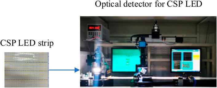
Figure 1. CSP LED automatic production line.

Defect detection is an essential stage in automated production quality assurance [8, 9]. In the automatic production line, the optical detector is a crucial component for ensuring the pass rate of CSP LED strips corresponding to the equipment in Figure 1. Generally, the number of dead beads is estimated based on the spacing between beads on trips. However, due to the small size of CSP-LED beads, there exist distance errors and angle errors between beads on CSP LED trips when the beads are packaged. Consequently, it is difficult to estimate the number of defective beads directly using bead distances in the CSP LED images.

The traditional methods for detecting defects in LED images primarily utilize image processing technologies, which are widely applied in many fields [10, 11]. It reconstructs the background of the LED image, detects the defect edges of beads, and subsequently segments defect targets. The primary procedures in defect detection include gathering elements with similar features into a single category, maximizing the element correlation in the same category, increasing the dissimilarity between elements from different categories, and finally dividing an image into several distinct parts [12]. Based on the above analysis, designing a defect detection method for CSP LED images is critical. Considering the above problems, Yang et al. [13] proposed an automatic segmentation method of thin-film transistor (TFT) liquid crystal display (LCD) images, focusing on multi-scale spatial information and significant defects. Jian et al. [14] explored solutions for automatically detecting surface defects on organic light-emitting diode (OLED) display screens by using the fuzzy C-means clustering-based defect detection (FD) method. Furthermore, the FD method was employed to calculate the membership degree of each element to all cluster centers by constructing a new function for each cluster element, classifying the samples based on the membership degree. [15] presented an effective method to process noisy images, effectively separating the background and defects. However, it may not perform optimally in the presence of image noises [16]. Considering the small size and large number of beads in a CSP LED strip, direct detection of defective beads on the strip using traditional the FD method proves challenging. Although deep learning can achieve satisfactory detection performance, its high hardware requirements often make it difficult to meet real-time inspection demands in production lines [17, 18].

Considering the advantages of neutrosophic theory in handling uncertain information, it has been introduced to enhance the accuracy of defect detection in noisy images, which is widely applied in the field of image processing [18, 19]. [20] applied neutrosophic in image edge detection, and further developed a neutrosophic clustering method [21]. Compared with fuzzy theory, neutrosophic theory offers a more objective approach for actual applications. Generally, the traditional fuzzy theory assesses whether an event meets a certain criterion by relying solely on truth and falsity as results. In contrast, neutrosophic theory defines a neutral region between truth and falsity [22, 23]. In recent years, the neutrosophic theory has also played an important role in the field of image processing, particularly for its capacity to effectively describe and process uncertain information in images. Due to the susceptibility of traditional image segmentation methods to noises, [24] proposed a neutrosophic image segmentation method based on local pixel grouping (LPG) and principal component analysis (PCA). The neutrosophic logic-based image segmentation method has been studied in [20]. The concept of kernel function based on neutrosophic theory has been introduced in [15, 25], extending these applications to fields such as medicine and remote sensing image processing. The neutrosophic theory has been adopted to detect dead knots in wood images [25]. A neutrosophic filtering method has been proposed for uncertain information fusion [26], effectively resolving the contradiction between high-density salt-and-pepper noise filtering and detail protection. In [27], an improved nonlocal prior image dehazing algorithm is presented by combining the fuzzy C-means clustering algorithm of neutrosophic theory with a hybrid dark channel prior transmittance optimization method.

Considered the influence of noises on defect detection, this paper utilizes the neutrosophic set-based defect detection method (ND) to detect defective beads on CSP LED images. It incorporates a similarity operation to handle image noises, and applies an enhancement operation to enhance image contrast. The effectiveness of the ND method is subsequently verified by a real-data experiment.

The remainder of this paper is organized as follows. Section 2 provides basic principle of neutrosophic theory, and it is employed to describe the uncertain information in CSP LED images. In Section 3, the neutrosophic set-based defect detection method is proposed. Section 4 presents the experimental results and the performance comparison with other five defect detection methods. Finally, the conclusions are provided in Section 5.

2 Basic principle of neutrosophic theory

This section introduces the basic principle of neutrosophic theory, and it will be used to describe the uncertainty in CSP LED images in Section 3. Assuming that $U$ denotes a non-empty set, a neutrosophic set $A$ is a subset of $U$, a vector $x\left(t,i,f\right)$ is an element in set $A$, where $t$, $i$ and $f$ is a variable in $T$, $I$ and $F$, respectively [28, 29]. $T$, $I$ and $F$ are standard or non-standard real subsets of $\left]-0,1+\right[$ and then

$\sup T=t_{\sup },\inf T=t_{\inf }(1)$

$\sup I=i_{\sup },\inf I=i_{\inf }(2)$

$\sup F=f_{\sup },\inf F=f_{\inf }(3)$

$n_{\sup }=t_{\sup }+i_{\sup }+f_{\sup }(4)$

$n_{\inf }=t_{\inf }+i_{\inf }+f_{\inf }(5)$

where $T$, $I$ and $F$ are the component of set $A$. $x_{\sup \left(x=t,i,f\right)}$ denotes the upper bound element in neutrosophic set $A$ while $x_{\inf \left(x=t,i,f\right)}$ denotes the lower bound element. The truth, indeterminacy and falsity membership of $x$ are denoted by $t$, $i$, $f$, respectively, and they correspond to the real value of the sets $T$, $I$ and $F$, respectively. The value of $t$, $i$, $f$ and their sum $n=t+i+f$ are not restricted [17, 20–32]. Here, $-0=0-\epsilon$, $1+=1+\epsilon$, “0” and “1” denote the standard part, while “$\epsilon$” represents the non-standard part, $\left]-0,1+\right[$ is the non-standard real sub-set.

3 Neutrosophic set-based defect detection methods

In real applications, there are slight deviations in the CSP LED beads’ dimensions and alignment, and the exposure time of detection images are different. Sometimes the boundaries of beads in images are blurred, and this results in the presence of numerous noises in CSP LED images. Then, we try to apply the uncertainty information of CSP LED images in the design of an defect detection method. Considering the advantages of neutrosophic set in processing uncertainty information, we have employed the ND method to detecting defective beads. In the ND method, firstly, CSP LED images are converted into neutrosophic images by using neutrosophic theory. Then, considering the presence of image noises, a similarity operation is applied to filter out noise pixels in neutrosophic images to make these images more uniform. Finally, an enhancement operation is implemented to improve image contrast. The main steps of the ND method are illustrated in Figure 2.

Figure 2

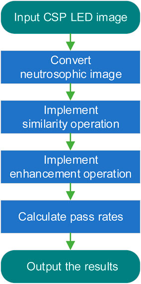
Figure 2. Main steps of the ND method.

3.1 Neutrosophic image converting

Suppose $U$ is a non-empty set, and $A$ is a set composed of values of all pixels in a CSP LED image, which is a subset of $U$. According to the neutrosophic theory, a CSP LED image consists of three parts: the truth part, indeterminacy part, and falsity part. Then, the image can be converted as a neutrosophic image $P_{NS}=\left\{T\left(i,j\right),I\left(i,j\right),F\left(i,j\right)\right\}$. Here, $T\left(i,j\right)$, $I\left(i,j\right),$ and $F\left(i,j\right)$ are a matrix. The main procedures of constructing the matrix $T\left(i,j\right)$, $I\left(i,j\right)$ and $F\left(i,j\right)$ is given as follows.

Firstly, a CSP LED image is input and converted into a grayscale image $g\left(i,j\right)$. Then, $G\left(i,j\right)$ is applied to calculate the regional mean value of this grayscale image by Equation 6.

$G\left(i,j\right)=\frac{1}{w\times w}{\displaystyle \sum _{m=i-\frac{2}{2}}^{i+\frac{w}{2}}}{\displaystyle \sum _{n=j-\frac{w}{2}}^{j+\frac{w}{2}}}g\left(m,n\right)(6)$

The converting process of the truth degree $T\left(i,j\right)$, the indeterminacy degree $I\left(i,j\right)$ and the falsity degree $F\left(i,j\right)$ can be expressed as

$T\left(i,j\right)=\frac{G\left(i,j\right)-g_{\min }}{g_{\max }-g_{\min }}(7)$

$I\left(i,j\right)=\frac{D\left(i,j\right)-D_{\min }}{D_{\max }-D_{\min }}(8)$

$F\left(i,j\right)=1-T\left(i,j\right)(9)$

Here, $g_{\max }$ and $g_{\min }$ represent the maximum gray value and minimum gray value in $g\left(i,j\right)$. $D\left(i,j\right)$ can be expressed by

$D\left(i,j\right)=\left|g\left(i,j\right)-G\left(i,j\right)\right|(10)$

where, $D\left(i,j\right)$ represents the absolute difference between $g\left(i,j\right)$ and $G\left(i,j\right)$ with $w=2n$, where $n$ is a positive integer. The value of w is different according to the difference in noise.

The pseudocode for the above steps can be represented as follows:

1. Let g be the image to be processed. If g is not in grayscale, convert it go grayscale.

2. Define w as the neighborhood diameter.

3. Create a matrix G of the same size as g.

4. Iterate over each pixel (i,j) in $g$ as follows:

- If the neighborhood with a radius of w/2 contains points that belong to the matrix, set G (i,j) to the mean of the w/2 neighborhood around the pixel.

- Otherwise set G (i,j) = g (i,j).

5. Create matrix T of the same size as g. Normalize it as Equation 7.

6. Generate matrix D of the same size as g. Calculate D as the absolute distance matrix between g and G at the corresponding pixel positions.

7. Create matrix I of the same size as g. Normalize it as Equation 8.

8. Produce matrix F with the same size as g. Define each pixel’s value in F as 1 minus the value of the corresponding pixel in T.

9. The matrices T, I and F together constitute the collection of neutrosophic images T, I and F.

3.2 Similarity operation

In general, similarity operation is utilized to assess the degree of similarity between two vectors. This is a common statistical model in the fields of data mining and signal processing. Due to the constraints in practical applications, there exist multiple methods for calculating similarity degrees. In this paper, we utilize the $\alpha$-similarity operation, and the primary implementation steps are given as follows.

First, one needs to establish the weight function $w\left(i,j,m,n\right)$, which represents the similarity degree between the gray values of the pixel $g\left(i,j\right)$ and the pixel $g\left(m,n\right)$ in an $\mathrm{\Omega }$ area. The weight function $w\left(i,j,m,n\right)$ primarily consists of the spatial weight function $c\left(i,j,m,n\right)$ and the domain weight function $s\left(i,j,m,n\right)$, which are employed to describe the spatial similarity degree and the domain similarity degree, respectively.

To choose the pixel $g\left(i,j\right)$ and the $\mathrm{\Omega }$ area around this pixel, it is necessary to adjust the values of $w$ according to the input image and the noises. Here, the value of the spatial weight function $c\left(i,j,m,n\right)$ takes the constant 1, that is

$c\left(i,j,m,n\right)=1(11)$

the domain weight function takes the similarity degree of the pixels, that is

$s\left(i,j,m,n\right)=\exp \left(-t\frac{{‖g\left(i,j\right)-g\left(m,n\right)‖}^2}{h^2}\right)(12)$

according to Equations 11, 12, we can get

$w\left(i,j,m,n\right)=c\left(i,j,m,n\right)s\left(i,j,m,n\right)(13)$

Then, $w\left(i,j,m,n\right)$ can be expressed by

$w\left(i,j,m,n\right)=\exp \left(-t\frac{‖g\left(i,j\right)-g\left(m,n\right)‖}{h^2}\right)(14)$

where

$g\left(i,j\right)=\frac{{\displaystyle {\sum }_m^w}{\displaystyle {\sum }_n^w}g\left(m,n\right)w\left(i,j,m,n\right)}{{\displaystyle {\sum }_m^w}{\displaystyle {\sum }_n^w}w\left(i,j,m,n\right)}(15)$

The process described above is often referred to as similarity operations. Here, $h>0$ is the smoothing parameter used to control the relative attenuation degree of the weight, while $t>0$ is the filter control parameter. Since the neutrosophic theory cannot eliminate the influence of pixel uncertainty on the detection result, the parameter $t$ can be taken as $t=2I\left(i,j\right)$, then the original weight function can be expressed as:

$s\left(i,j,m,n\right)=\exp \left(-2I\left(i,j\right)\frac{{‖g\left(i,j\right)-g\left(m,n\right)‖}^2}{h^2}\right)(16)$

Here, the radius of each pixel neighborhood is $w$. When determining the value of the pixel $p\left(i,j\right)$ based on the values of its surrounding pixels, it is essential to account for the possibility that $p\left(i,j\right)$ may be a noise pixel. Therefore, the neutrosophic set $I\left(i,j\right)$ is employed to describe the uncertainty of a pixel. If the values in the neighborhood of pixel $p\left(i,j\right)$ are generally high when assessed with $I\left(i,j\right)$, $p\left(i,j\right)$ is likely to be a noisy pixel. In such a case, its impact on the surrounding pixels should be reduced to a certain extent.

According to the neutrosophic theory, each image inherently contains a degree of uncertainty. When using the similarity operation and selecting the uncertainty $I\left(i,j\right)$ as the decision criterion, it is essential to establish a threshold $\alpha$ to prevent overprocessing and avoid categorizing non-noisy points as noise points. When $I\left(i,j\right)\ge \alpha$, the point is processed according to the steps described above; when $I\left(i,j\right)<\alpha$, it is left unprocessed. The series of steps is referred to as the $\alpha$-similarity operation. In this paper, considering the practical situation, the threshold value $\alpha$ is defined as 0.85. Consequently, a new neutrosophic set $Tba$ and $Iba$ can be described as follows:

$Iba=\left\{\begin{array}{l}T\\ Tba2\end{array}\right.\begin{array}{l}I<\alpha \\ I\ge \alpha \end{array}(17)$

$G\left(i,j\right)=\frac{{\displaystyle {\sum }_{m=i-\frac{w}{2}}^{i+\frac{w}{2}}}{\displaystyle {\sum }_{n=j-\frac{w}{2}}^{j+\frac{w}{2}}}T\left(m,n\right)w\left(i,j,m,n\right)}{{\displaystyle {\sum }_{m=i-\frac{2}{2}}^{i+\frac{w}{2}}}{\displaystyle {\sum }_{n=j-\frac{w}{2}}^{j+\frac{w}{2}}}w\left(i,j,m,n\right)}(18)$

$Tba2\left(i,j\right)=\frac{1}{w\times w}{\displaystyle \sum _{m=i-\frac{2}{2}}^{i+\frac{w}{2}}}{\displaystyle \sum _{n=j-\frac{w}{2}}^{j+\frac{w}{2}}}Tba\left(i,j\right)(19)$

$Dba\left(i,j\right)=\left|Tba\left(i,j\right)-Tba2\left(i,j\right)\right|(20)$

$Iba\left(i,j\right)=\frac{Dba\left(i,j\right)-Db{a}_{\min }}{Db{a}_{\max }-Db{a}_{\min }}(21)$

where, D (i,j) is the absolute difference between g (i,j) and G (i,j), w = 2n, where $n$ is a positive integer, and the value range of w varies depending on the level of noises.

The pseudocode for the $\alpha$-similarity operation is provided below:

1. Define the following variables:

- $g$: the original image matrix; $T$: the neutrosophic image collection $T$; $I$: the neutrosophic image collection $I$; $F$: the neutrosophic image collection $F$; $L$: the radius of the pixel’s neighborhood; $h$: the smoothing parameter; $\alpha$: the threshold; $Ta1$: a matrix of the same size as the original image; $Ta2$: a matrix of the same size as the original image; $Iba$: the normalized matrix $Dba$.

2. Process each pixel (i,j) sequentially in $g$ as follows:

- Check if a pixel’s neighborhood with a radius of L/2 contains only pixels belong to the matrix.

- If does, perform the following calculations for each pixel in the neighborhood:

- Calculate Ta1 (i,j) using the formula exp $\left(-2I\left(m,n\right){\left(T\left(i,j\right)-T\left(m,n\right)\right)}^2/h^2\right)$.

- Calculate Ta2 (i,j) using the formula T (m, n) exp$\left(-2I\left(m,n\right){\left(T\left(i,j\right)-T\left(m,n\right)\right)}^2/h^2\right)$.

- Calculate Ta (i,j) by dividing the corresponding pixel of Ta2 (i,j) by the pixel of Ta1 (i,j) in the same position.

- Otherwise, set Ta (i,j) to the corresponding pixel in T.

3. Generate matrix Tba of the same size as the original image.

- If the pixels in I are greater than or equal to the threshold $\alpha$, set the pixels in Tba to correspond to the pixels in Ta.

- Otherwise, set the pixels in Tba to correspond to the pixels in T.

4. Generate a matrix Tba2 as the same size of the original image.

- Process each pixel sequentially in g.

- If the L/2 neighborhood of the pixel contains the pixels that belong to the matrix, calculate the mean value of the pixels in the L/2 neighborhood corresponding to T.

- Otherwise, set the pixels in Tba2 to be equal to the corresponding pixels in T.

5. Calculate $Dba$ as the absolute distance matrix between Tba and Tba2.

6. Normalize matrix Dba to create Iba by Equation 21.

7. $Iba$ represents the image after the $\alpha$-similarity operation.

3.3 Enhancement operations

After converting the neutrosophic image and performing the similarity operation, the outline of CSP LED image may become blurred. This blurriness is not conducive to subsequent processing. Therefore, it is necessary to enhance the image through the enhancement operation method to increase the contrast of images. This will result in clearer detected edges. The formula for the enhancement operation is as follows:

$Ib{a}^{\prime }\left(i,j\right)=\left\{\begin{array}{l}2Ib{a}^2\left(i,j\right)\\ 1-2\left(1-Ib{a}^2\left(i,j\right)\right)\end{array}\right.\begin{array}{l}Iba\left(i,j\right)<\beta \\ Iba\left(i,j\right)\ge \beta \end{array}(22)$

Here, a threshold ß is set to 0.5. Different operations can be performed based on the pixel values in Iba and compared to ß.

4 Experiment results and analysis

The experiments using actual CSP LED images have been conducted to verify the effectiveness of the neutrosophic set-based defect detection (ND) method when compared to the other five defect detection methods as follows: the direct defect detection (D2), low-pass filter-based defect detection (LD) [33], Gaussian filter-based defect detection (GD) [34], mean filter-based defect detection (MD) [35], fuzzy C-means clustering-based defect detection (FD) [15], and the proposed neutrosophic set-based defect detection (ND) method. As illustrated in Figure 3, these CSP LED images with varying exposure times were captured by using an industrial camera (type: Hikvision MV-CA060-11GM; exposure time range: 27 μs–2.5 s) integrated into the optical detector in automatic production line as Figure 1. This equipment was sourced from [36]. To illustrate the reliability of the detection results, we employ the images with six exposure times and compare their detection results. The experiments were carried out on a computer with a dual-core CPU of Core Intel(R) Xeon(R) E5-26650 at 2.40 GHz with 32-GB of RAM. The programs for the above six detection methods were implemented by using MATLAB R2023a version software.

Figure 3

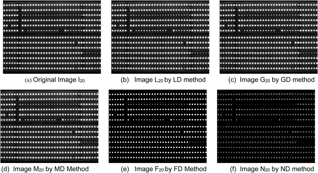
Figure 3. CSP LED images by six detection methods. (a) Original Image I₂₀ (b) Image L₂₀ by LD method (c) Image G₂₀ by GD method. (d) Image M₂₀ by MD Method (e) Image F₂₀ by FD Method (f) Image N₂₀ by ND method.

4.1 Defect detection of CSP LED images

In this section, six detection methods mentioned above have been applied to detect defective beads in CSP LED images. Figure 3a displays the original CSP LED image I₂₀, and Figures 3b–f show the detection results obtained by using the LD method, GD method, MD method, FD method and ND method, respectively. Despite the presence of noises in Image I₂₀, which impact detection results at certain degrees, it is evident from the detection results by Figure 3e and f that both the FD method and ND method can accurately detect the beads. We will illustrate these detection results in the following sections. However, the distribution of gray values in Image N₂₀ is more uniform compared to Image F₂₀. This is because the ND method incorporates the neutrosophic set to describe the uncertain information in CSP LED images and utilizes the information effectively. Hence, it can suppress the noises’ impact.

To assess the robustness of the ND method, we can further apply the other CSP LED images with different contrasts in six exposure times as shown in Table 1 and Figures 4–9. Generally, the shorter the exposure time, the darker and the higher the contrast. In other words, the longer the exposure time, the brighter and the lower the contrast. In actual applications, if the contrast of CSP LED images is lower, it is more difficult to detect defective beads. Based on this fact, we need to select not only CSP images in the right exposure times, but also conveyor belt speed is an important factor, which influenced the choice of exposure times. Here, Figures 4–9 show the original images and the processed images by the corresponding LD, GD, MD, FD and ND method. From Figures 4–9, it is observable from Figure 9 that the ND method can yield the more robust detection results consistently, even with extended exposure time. In other words, it is not significantly affected by the noises. As a result, the ND method can provide an effective solution to the defect detection challenges in CSP-LED images.

Table 1

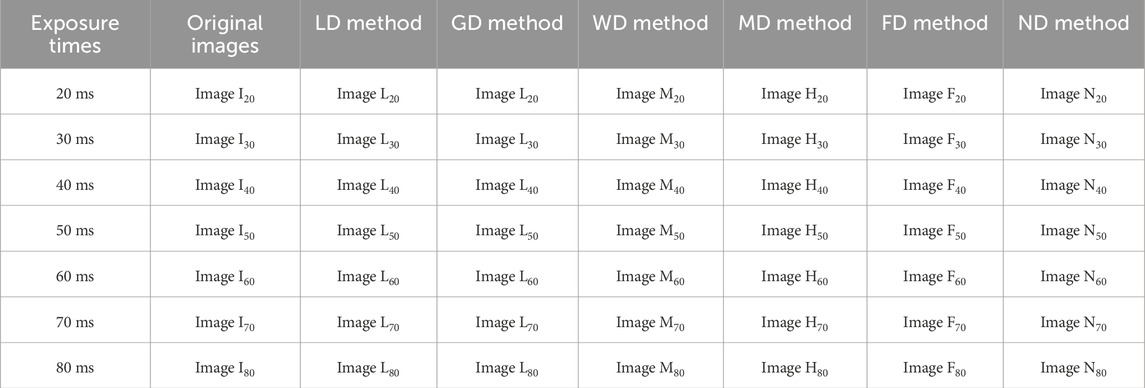
Table 1. Exposure times for CSP LED images.

Figure 4

Figure 4. Orginal images. (a) I₃₀. (b) I₄₀. (c) I₅₀. (d) I₆₀. (e) I₇₀. (f) I₈₀.

Figure 5

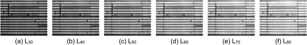
Figure 5. Results by the LD method. (a) L₃₀. (b) L₄₀. (c) L₅₀. (d) L₆₀. (e) L₇₀. (f) L₈₀.

Figure 6

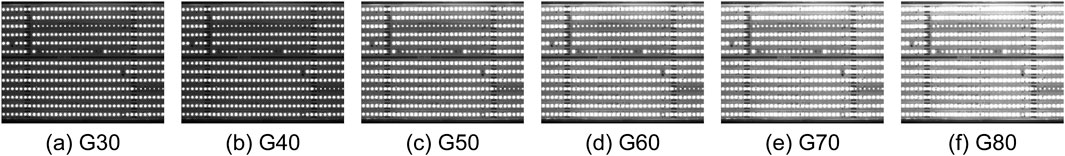
Figure 6. Results by the GD method. (a) G30. (b) G40. (c) G50. (d) G60. (e) G70. (f) G80.

Figure 7

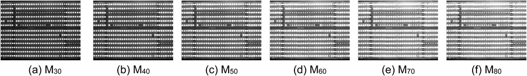
Figure 7. Results by the MD method. (a) M₃₀. (b) M₄₀. (c) M₅₀. (d) M₆₀. (e) M₇₀. (f) M₈₀.

Figure 8

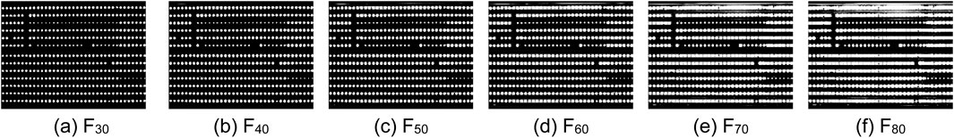
Figure 8. Results by the FD method. (a) F₃₀. (b) F₄₀. (c) F₅₀. (d) F₆₀. (e) F₇₀. (f) F₈₀.

Figure 9

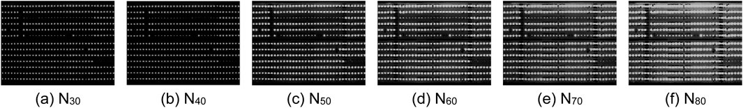
Figure 9. Results by the ND method. (a) N₃₀. (b) N₄₀. (c) N₅₀. (d) N₆₀. (e) N₇₀. (f) N₈₀.

For quantitative analysis of the proposed ND method, we further list the following five statistical features of filtering images by these detection methods compared with the original images. Concretely, these statistical features include the mean, standard deviation, entropy, gradient magnitude and structural similarity index (SSID) measure, respectively. As a result, we can obtain the variations of five features between the filtered images and original images as Table 1, calculated by the following equations, respectively.

$\mu \left(X\right)=\frac{1}{MN}{\displaystyle \sum _{i=1}^M}{\displaystyle \sum _{j=1}^N}X\left(i,j\right)(23)$

$\sigma \left(X\right)=\sqrt{\frac{1}{MN}{\displaystyle \sum _{i=1}^M}{\displaystyle \sum _{j=1}^N}{\left(X\left(i,j\right)-\mu \right)}^2}(24)$

$H\left(X\right)=-{\displaystyle \sum _{i=0}^{Level}}p\left(i\right){\log }_2^{p\left(i\right)}(25)$

$g\left(X\right)=\sqrt{{\left(\frac{\mathrm{\partial }X}{\mathrm{\partial }x}\right)}^2+{\left(\frac{\mathrm{\partial }X}{\mathrm{\partial }y}\right)}^2}(26)$

$s\left(X,Y\right)=\frac{\left(2\mu \left(X\right)\mu \left(Y\right)+C_1\right)\left(2\sigma \left(X,Y\right)+C_2\right)}{\left({\mu }^2\left(X\right)+{\mu }^2\left(Y\right)+C_1\right)\left({\mu }^2\left(X\right)+{\mu }^2\left(Y\right)+C_2\right)}(27)$

Here, μ, σ, H, g and s represent the mean, standard deviation, entropy, gradient magnitude and SSIM, respectively. X and Y denote gray images with dimensions M rows by N columns. To prevent division by zero, small positive constants C₁ and C₂ are incorporated into the SSIM in Equation 27. The probability of gray level i, denoted as p(i), is calculated for each gray level from i = 1 to Level = 255 as defined in Equation 28.

$p\left(i\right)=\frac{n\left(i\right)}{M\times N}(28)$

From Table 2, the proposed ND method achieves relatively high μ, σ values, significant g value, moderate H value, and comparatively low s value. These results show its enhanced sensitivity and accuracy in detecting defects. Meanwhile, the ND method exhibits a notable advantage in balancing detection performance. It is beneficial for identifying defects within CSP LED images. Based on the comparison of the variations of five features in Table 1, the variation in SSID by the ND method is close to that by the FD, and their results in five features are better than other detection methods. However, the FD method makes significant changes overly in gray values, and it actually leads to a decrease in defect detection capabilities, which will be analyzed in Section 4.2. For more intuitive illustration, the above results in standard deviation and SSID are further illustrated in Figures 10a,b. From Figures 10a,b, we can observe that the curves corresponding to the two types of image features align the above results, and follow a consistent pattern of either rising or falling with the exposure time changes.

Table 2

Table 2. Image statistical features for each detection method.

Figure 10

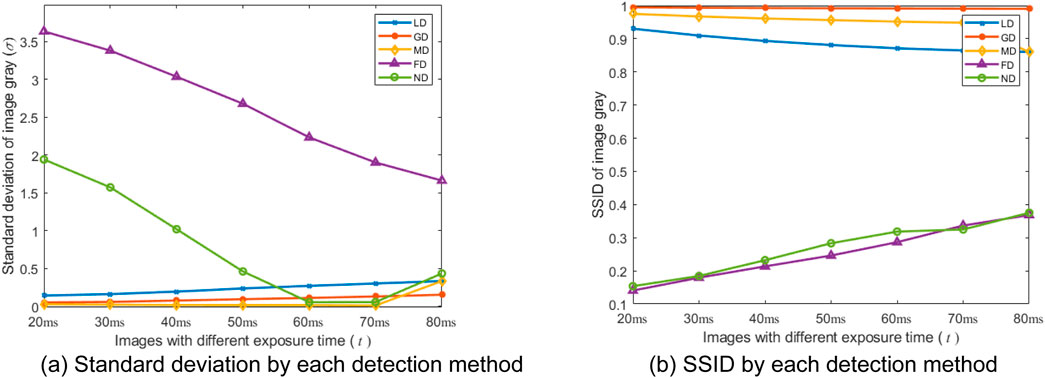
Figure 10. Two statistical features for each detection method. (a) Standard deviation by each detection method. (b) SSID by each detection method.

4.2 Calculation and analysis of pass rate

Based on Section 4.1, the filtered images and original images can be obtained using six detection methods. Then, the pixel position (i,j) of a bead in CSP LED images can be calculated in the following procedure, and its pass status depends on its gray value g (i,j). Here, the gray value denotes the color depth of a pixel, ranging from 0 to 255, where 0 indicates black. Generally, the pixel positions of beads in CSP LED images exhibit uniform and regular patterns, similar to a chessboard, as shown in Figure 3. Then, the gray values of a CSP LED image can be summed along its rows and columns, respectively. Concretely, this procedure identifies peaks with row x by column y as shown in Figures 11, 12. Finally, the peak establishes the real bead by (i_b,j_b). In the procedure, if the gray value of the bead (i_b,j_b) is less than the given gate g_f, the bead is defective.

Figure 11

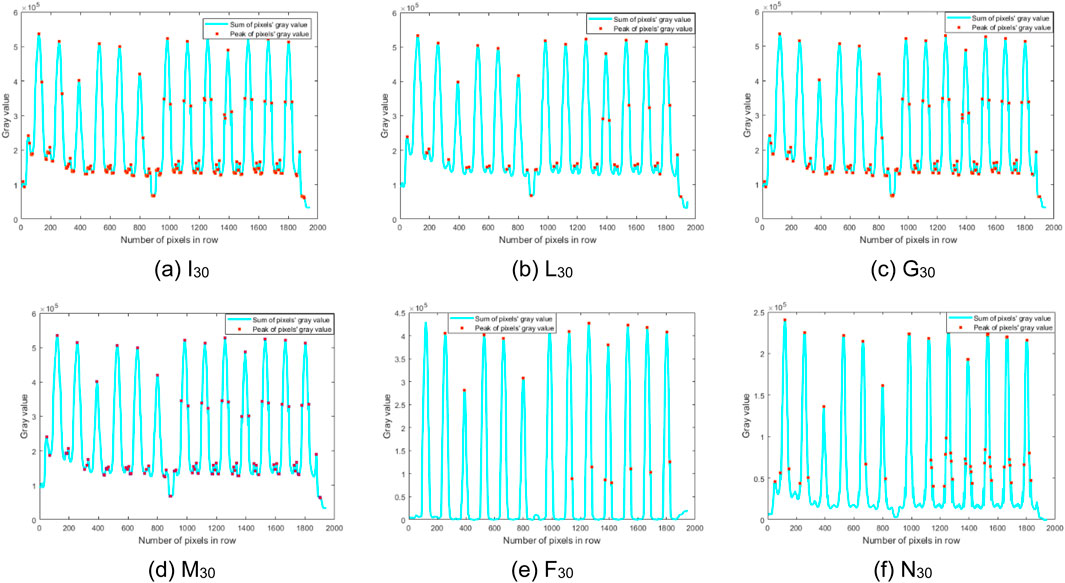
Figure 11. Peaks in a row. (a) I₃₀. (b) L₃₀. (c) G₃₀. (d) M₃₀. (e) F₃₀. (f) N₃₀.

Figure 12

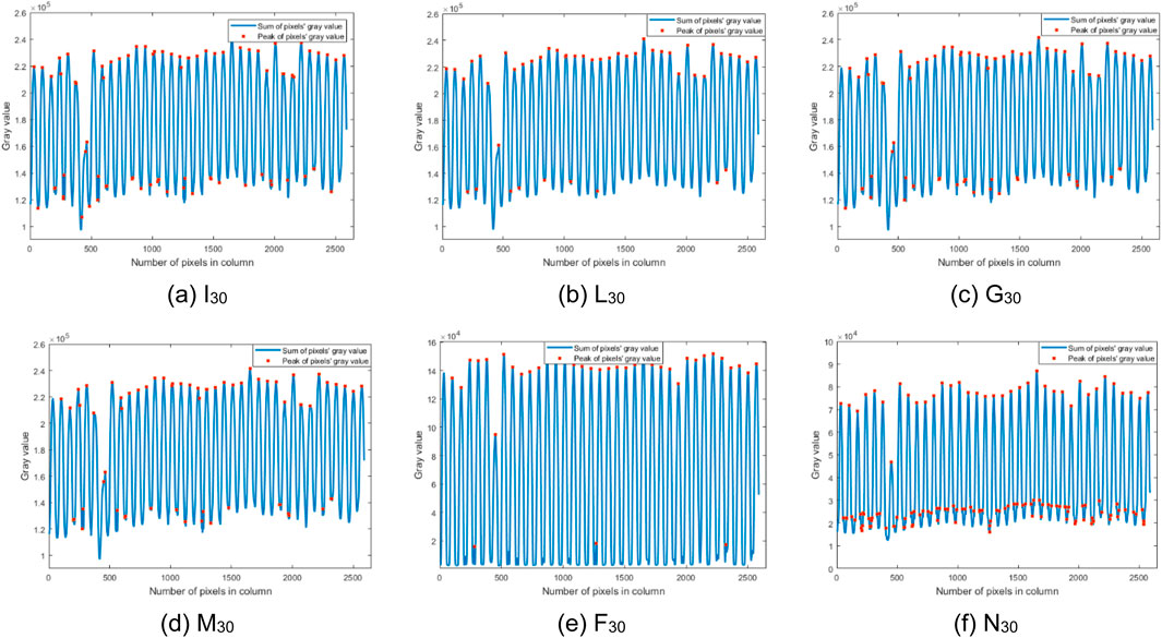
Figure 12. Peaks in a column. (a) I₃₀. (b) L₃₀. (c) G₃₀. (d) M₃₀. (e) F₃₀. (f) N₃₀.

From Figures 11, 12, the waveforms of the ND method are shaper, and its gray values are more concentrated (0–2.5 × 10⁵ for x, 0–1.0 × 10⁴ for y) than those of other five images. The peak positions in Image N₂₀ are more accurate than those by other five detection methods. Moreover, some false peaks are present in Figure 12a, while some real peaks are not detected in Figures 12c–e. Consequently, the images filtered by the ND method are more accurate to detect the defective beads. This is due to the presence of noises in the CSP LED images, and the ND method can suppress the noise at certain degree by incorporating the neutrosophic set to model uncertain information. It will be further analyzed below. Therefore, the detection performance of the ND method is the best in six images. Additionally, the number N_b of beads in an image can be calculated by

$N_b=n_x\times n_y(29)$

where the numbers n_x and n_y represent the peaks in a row and a column, respectively. Here, they can be easily estimated as n_x = 13 and n_y = 37 by six methods for all images from Figures 11, 15, and then N_b = 481 estimated.

Tables 3, 4 further summarize the detection performance of six methods under two optimal and fixed detection thresholds, respectively. For the purpose of analysis, three metrics are defined: the estimated pass rate r_p, the real pass rate r_po and the fault detection rate r_f. They can be further represented as follows:

$r_p=\left(N_b-n_d\right)/N_b(30)$

$r_{po}=\left(N_b-n_r\right)/N_b(31)$

$r_f=\left|r_p-r_{po}\right|(32)$

where n_d is the estimated number of the defective beads in a CSP LED image, n_r is the real number of the defective beads, N_b is the total number of all beads mentioned in Section 4.1. Here, g_d represents the given gray gate in Tables 3, 4, n_r = 10 and n_b = 481. Based on the definitions above, the estimated pass rate r_p represents the ratio of the detected number N_b-n_d of pass beads to the total number N_b of all beads. Similarly, the real pass rate r_p is the ratio of the real number N_b-n_r of pass beads to the total number N_b of all beads. The fault detection rate r_f indicates the difference between the estimated pass rate r_p and the real pass rate r_po.

Table 3

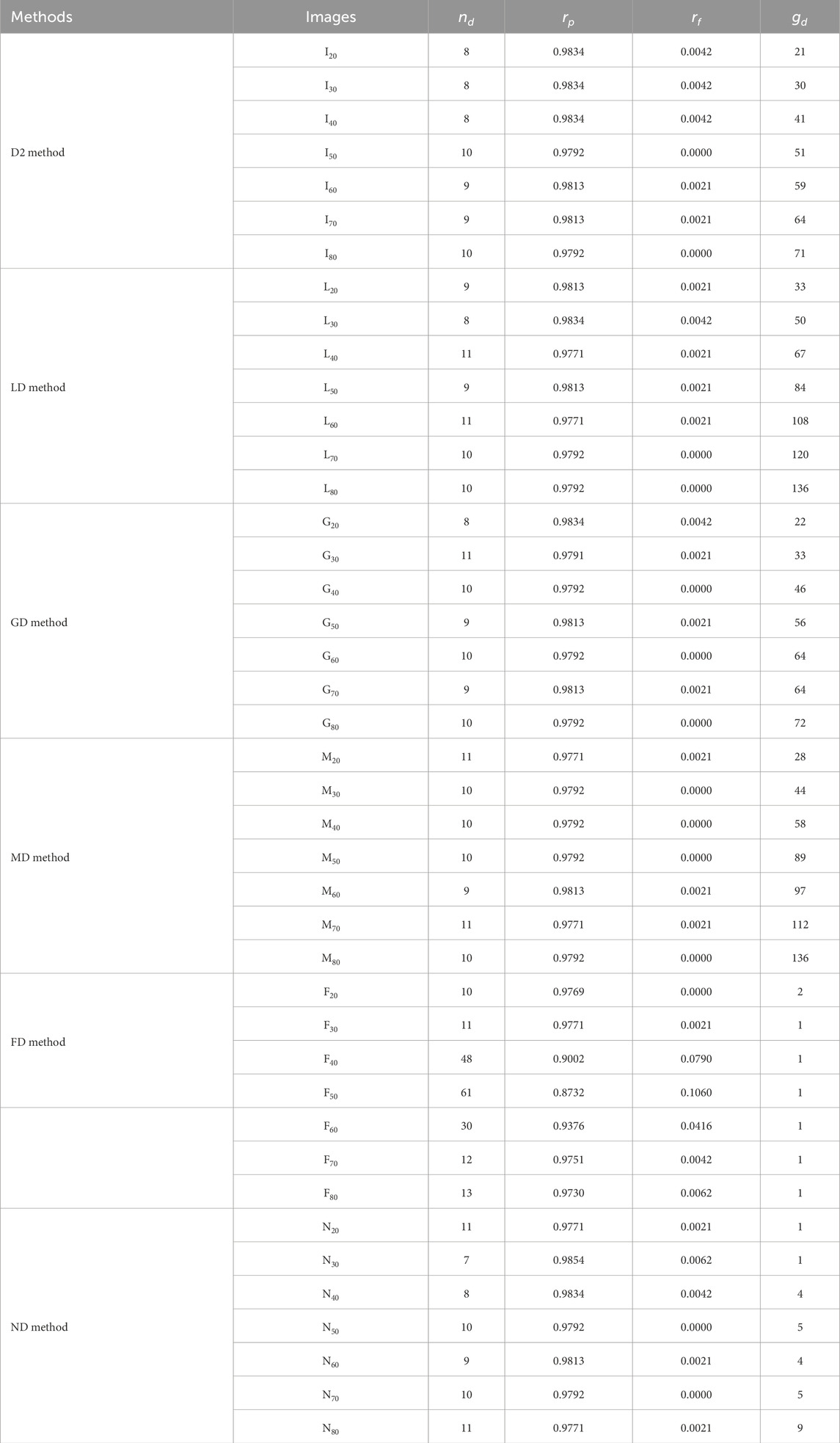
Table 3. Detection performances of six detection methods under optimal detection thresholds.

Table 4

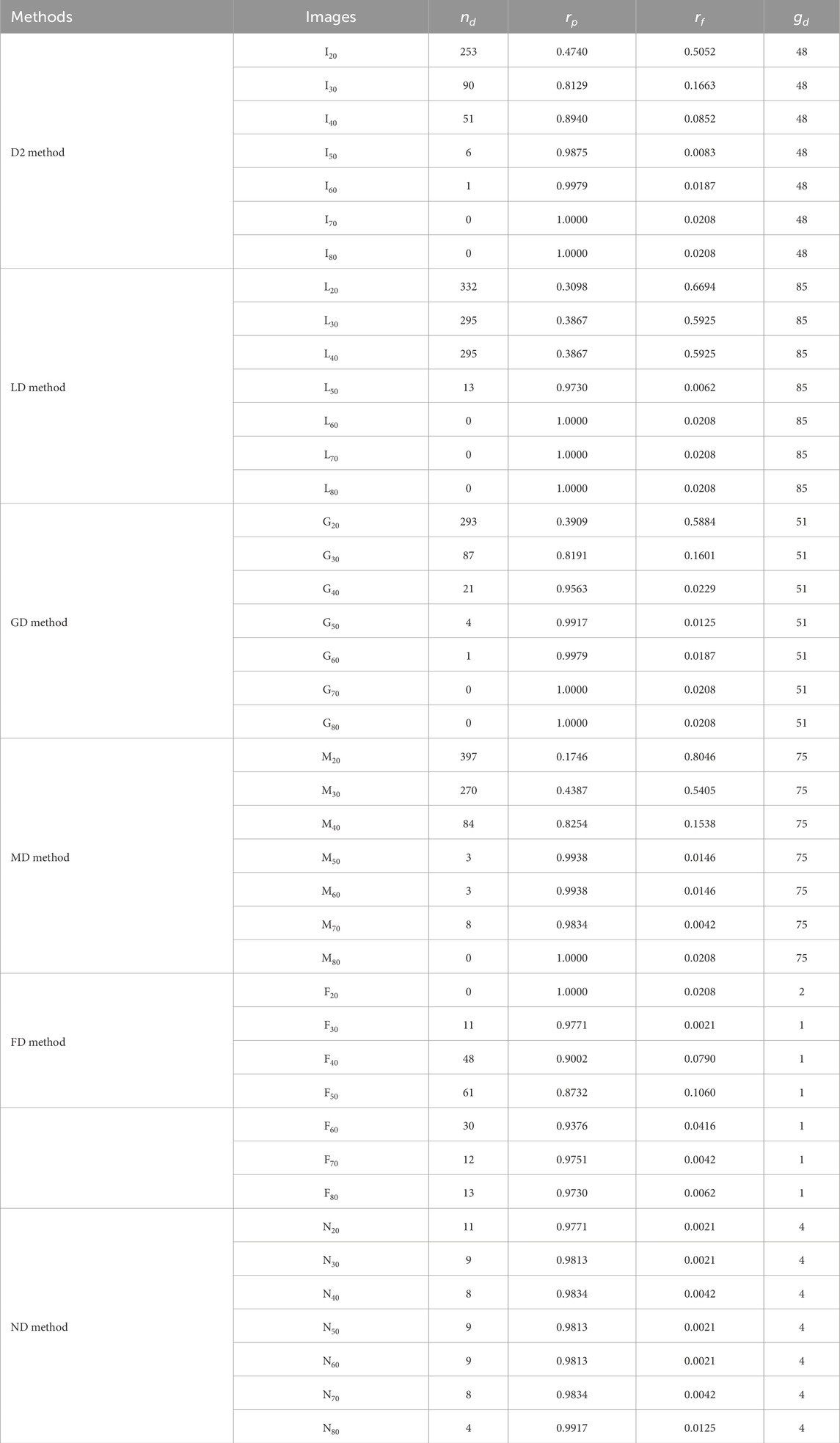
Table 4. Detection performances of six detection methods under fixed detection thresholds.

From Table 3, five detection methods except for FD method yield good detection results for different images with optimal detection thresholds. Here, the optimal detection thresholds for six methods are determined by the traversal tests within the threshold range from 1 to 160. Generally, a smaller fault detection rate indicates better performance for a detection method. The first five methods exhibit slightly better detection performance than the FD method under the optimal detection thresholds, but the optimal detection thresholds of the ND method are more stable than those for other five detection methods. The FD method has the stable detection thresholds but the unsatisfied detection results for different images. Meanwhile, Figure 13 is applied to illustrate this fact. Unfortunately, determining the optimal detection thresholds dynamically in real applications is challenging, generally, requiring the fixed detection thresholds for each detection. Hence, we further analyze the detection performance of six methods under the fixed detection thresholds. In Table 4, the fixed detection thresholds are determined by multiple experiments to guarantee the good detection results for different images. Under the fixed detection thresholds, the ND method obtains the best detection performance among the six methods according to the fault detection ratio in Table 4. Moreover, Figure 14 provides further clarification of this fact.

Figure 13

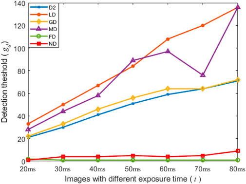
Figure 13. Fault detection rate by each detection method for different images.

Figure 14

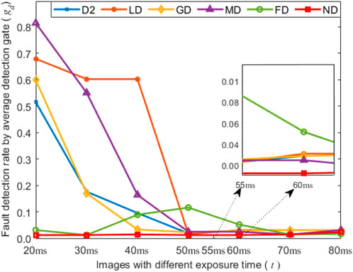
Figure 14. Optimal detection thresholds by fixed detection gates.

Figure 15 provides an intuitive comparison of the impact of varying detection thresholds on six methods by illustrating the number of defective beads using six methods. From Figure 14, we can identify the optimal detection thresholds for each detection method, which are consistent with the values presented in Tables 3, 4. Notably, the number of defective beads detected by the ND method is very close to the real number of defective beads, which corresponds to the red line and the black line, respectively. The D2, LD, MD and GD method outperform quite closely but not well from the threshold 30 to 35, while their detection results become worse after the threshold 30. In addition, if the detected number of defective beads by a detection method is equal to zero, it illustrates that the detection method fails to detect the defective beads under the corresponding threshold. Then, from the threshold 1 to 30, the D2, LD, MD and GD method fail to detect the defective beads. This analyzed result is nearly consistent with the preceding analysis.

Figure 15

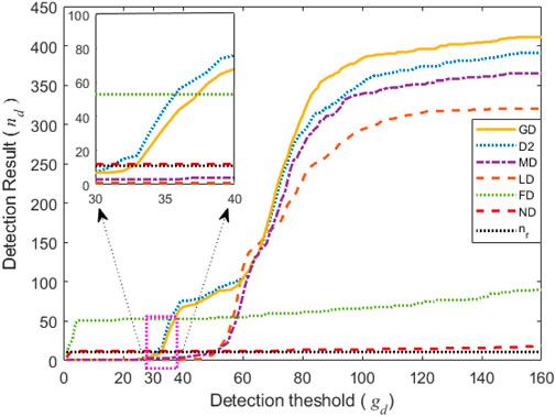
Figure 15. Number of defective beads detected by six detection methods under different thresholds.

On the whole, the detection performance of the ND method surpasses that of other five methods for the images with exposure time. Its detection performance remains more robust in situations with both optimal and fixed detection thresholds.

5 Conclusion

In actual applications, the detection of defective beads in CSP LED trips poses a significant challenge due to various noises and uncertain factors. This fact increases the complexity of the traditional defect detection methods, often resulting in fault detection. Considering the specific characteristics of CSP LED images, including high precision and small size, we employed the ND method to detect defective beads in CSP LED images. This approach is beneficial to improve the robust and accuracy of defective beads detection on CSP LED strips in automated production lines. Moreover, the ND method incorporates a similarity operation to address image noise and utilizes an enhancement operation to improve image contrast. Experimental results show the effectiveness of the ND method in detecting defective beads in CSP LED images, even in the presence of noise and complex backgrounds. Additionally, it accurately estimates the pass rate of LED CSP images when compared to five traditional defect detection methods.

In the following research, we will study the adaptive detection thresholds to further enhance detection accuracy of the proposed ND method in pass rate.

Data availability statement

The original contributions presented in the study are included in the article/supplementary material, further inquiries can be directed to the corresponding author.

Author contributions

EF: Writing – original draft. JG: Writing – review and editing. ZW: Writing – review and editing, Formal Analysis. QL: Writing – review and editing. CF: Writing – review and editing, Visualization.

Funding

The author(s) declare that financial support was received for the research and/or publication of this article. This work was financially supported by the National Natural Science Foundation of China (No. 62272311), and the Natural Science Foundation of Zhejiang Province (No. LGG22F010004).

Acknowledgments

This work was supported by Grandseed Science & Technology Co. Ltd. through the provision of proprietary industry data.

Conflict of interest

The authors declare that the research was conducted in the absence of any commercial or financial relationships that could be construed as a potential conflict of interest.

Generative AI statement

The author(s) declare that no Generative AI was used in the creation of this manuscript.

Publisher’s note

All claims expressed in this article are solely those of the authors and do not necessarily represent those of their affiliated organizations, or those of the publisher, the editors and the reviewers. Any product that may be evaluated in this article, or claim that may be made by its manufacturer, is not guaranteed or endorsed by the publisher.

References

1. Xie L, Chu Z, Li Y, Gu T, Wang C, Lu S, et al. Industrial vision: rectifying millimeter-level edge deviation in industrial internet of things with camera-based edge device. IEEE Trans Mobile Comput (2023) 23(3):1–17. doi:10.1109/tmc.2023.3246176

CrossRef Full Text | Google Scholar

2. Fabrucui MA, Behrens FH. Monitoring of industrial electrical equipment using IoT. IEEE Latin America Trans (2020) 18(8):1548–432.

Google Scholar

3. Zhu H, Huang J, Liu H, Zhou Q, Li B. Deep-learning-enabled automatic optical inspection for module-level defects in LCD. IEEE Internet Things J (2021) 9(2):1122–35. doi:10.1109/jiot.2021.3079440

CrossRef Full Text | Google Scholar

4. Zhang Y, Wang W, Wu N, Qian C. IoT-enabled real-time production performance analysis and exception diagnosis model. IEEE Trans Automation Sci Eng (2015) 13(3):1318–32. doi:10.1109/tase.2015.2497800

CrossRef Full Text | Google Scholar

5. Chen C, Zhao D, Xiong Z, Niu Y, Sun Z, Xiao W. Comparative study of the photoelectric and thermal performance between traditional and chip-scale packaged white LED. IEEE Trans Electron Devices (2021) 68(4):1710–6. doi:10.1109/ted.2021.3058091

CrossRef Full Text | Google Scholar

6. Jiang B, Liu H, Zou J, Li W, Shi M, Yang B, et al. Packaging design for improving the uniformity of chip scale package (CSP) LED luminescence. Microelectronics Reliability (2021) 122:114136. doi:10.1016/j.microrel.2021.114136

CrossRef Full Text | Google Scholar

7. Tang B, Fan E, Li X. Web management platform design for CSP-LED production lines. Scientific Technol Innovation (2022) 32:17–20.

Google Scholar

8. Wang H, Hou Y, He Y, Wen C, Giron-Palomares B, Duan Y. A physical-constrained decomposition method of infrared thermography: pseudo restored heat flux approach based on ensemble Bayesian variance tensor fraction. IEEE Trans Ind Inform (2024) 20(3):3413–24.

CrossRef Full Text | Google Scholar

9. Li X, Wang H, He Y, Gao Z, Zhang X, Gao Z, et al. Active thermography nondestructive testing going beyond camera’s resolution limitation: a heterogenous dual-band single-pixel approach. IEEE Trans Instrumentation Meas (2024) 74:1–8. doi:10.1109/tim.2025.3545520

CrossRef Full Text | Google Scholar

10. Liu Y, Wang C, Wen Y, Huo Y, Liu J. Efficient segmentation algorithm for complex cellular image analysis system. IET Control Theor and Appl (2023) 17(17):2268–79. doi:10.1049/cth2.12466

CrossRef Full Text | Google Scholar

11. Han X, Chen Q, Ma Q, Yang X, Men H, Su Y, et al. Depth hole filling and optimizing method based on binocular parallax image. IET Control Theor and Appl (2023) 17(15):2064–70. doi:10.1049/cth2.12425

CrossRef Full Text | Google Scholar

12. Li Q, Zheng H, Cui T, Zhang Y. Identification and location method of strip ingot for autonomous robot system using k-means clustering and color segmentation. IET Control Theor and Appl (2023) 17(16):2124–35. doi:10.1049/cth2.12481

CrossRef Full Text | Google Scholar

13. Yang Q, Zhao YQ, Zhang F. Automatic segmentation of defect in high-precision and small-field TFT-LCD images. Laser and Optoelectronics Prog (2022) 12:314–21.

Google Scholar

14. Jian C, Wang H, Xu J, Su L, Wang T. Automatic surface defect detection for OLED display. Packaging Eng (2021) 13:280–7.

Google Scholar

15. Cui X, Wu C. Neutrosophic C-means clustering in kernel space and its application in image segmentation. J Image Graphics (2016) 10:1316–27.

Google Scholar

16. Yu H. On combining deep features and machine learning for automatic edge pedestrian detection task. Internet Technology Lett (2022) 6:1–6. doi:10.1002/itl2.356

CrossRef Full Text | Google Scholar

17. Jia Y, Chen G, Zhao L. Defect detection of photovoltaic modules based on improved VarifocalNet. Scientific Rep (2024) 14(1):15170. doi:10.1038/s41598-024-66234-3

PubMed Abstract | CrossRef Full Text | Google Scholar

18. Huang Z, Zhang C, Ge L, Chen Z, Lu K, Wu C. Joining spatial deformable convolution and a dense feature pyramid for surface defect detection. IEEE Trans Instrumentation Meas (2024) 73:1–14. doi:10.1109/tim.2024.3370962

CrossRef Full Text | Google Scholar

19. Hu K, Fan E, Ye J, Shen S, Gu Y. A method for visual foreground detection using the correlation coefficient between multi-criteria single valued neutrosophic multisets. Chin J Sensors Actuators (2018) 5:738–45.

Google Scholar

20. Guo Y, Sengur A. A novel image edge detection algorithm based on neutrosophic set. Comput and Electr Eng (2014) 40(8):3–25. doi:10.1016/j.compeleceng.2014.04.020

CrossRef Full Text | Google Scholar

21. Ashour A, Guo Y, Kuçukkulahli E, Erdogmuş P, Polat K. A hybrid dermoscopy images segmentation approach based on neutrosophic clustering and histogram estimation. Appl Soft Comput (2018) 69:426–34.

CrossRef Full Text | Google Scholar

22. AboElHamd E, Shamma H, Saleh M, El-Khodary I. Neutrosophic logic theory and applications. Neutrosophic sets Syst (2021) 41(1):30–51.

Google Scholar

23. Zhao R, Luo M, Li S. Reverse triple I method based on single valued neutrosophic fuzzy inference. J Intell and Fuzzy Syst (2020) 39(5):7071–83. doi:10.3233/jifs-200265

CrossRef Full Text | Google Scholar

24. Zhang G, Wang D. Neutrosophic image segmentation approach integrated LPG&PCA. J Image Graphics (2014) 5:693–700.

Google Scholar

25. Zhou Y, Pan S, Liu W, Yu Y, Zhou K, Liu J. Wood defect image detection method based on neutrosophic sets. For Machinery and Woodworking Equipment (2020) 10:64–8.

Google Scholar

26. Qi X, Liu B, Xu J. A novel algorithm for removing high-density salt-and-pepper noise based on fusion of indeterminacy information. Acta Electronica Sinica (2016) 4:878–85.

Google Scholar

27. Yu K, Jiao Q, Liu Z. Non-local prior image dehazing algorithm based on neutrosophy. Opt Tech (2020) 4:476–82.

Google Scholar

28. Ye J, Song J, Du S. Correlation coefficients of consistency neutrosophic sets regarding neutrosophic multi-valued sets and their multi-attribute decision-making method. Int J Fuzzy Syst (2022) 24:925–32. doi:10.1007/s40815-020-00983-x

CrossRef Full Text | Google Scholar

29. Ye J, Cui W. Exponential entropy for simplified neutrosophic sets and its application in decision making. Entropy (2018) 20. doi:10.3390/e20050357

PubMed Abstract | CrossRef Full Text | Google Scholar

30. Zhao X, Wang S, Liu Y. Neutrosophic image segmentation approach based on similarity. Appl Res Comput (2012) 6:2371–4.

Google Scholar

31. Yu Z, He L, Wang Z. Image edge detection based on intelligence theory and direction α-mean. J Electron Meas Instrumentation (2020) 3:43–50.

Google Scholar

32. Qi X, Liu B, Xu J. Impulse noise removal algorithm based on the fusion of directional characteristic and indeterminacy information. J Image Graphics (2017) 6:754–66.

Google Scholar

33. Su Y. An analytical study on the low-pass filtering effect of digital image correlation caused by under-matched shape functions. Opt Lasers Eng (2023) 168. doi:10.1016/j.optlaseng.2023.107679

CrossRef Full Text | Google Scholar

34. Fu WL, Johnston M, Zhang MJ. Genetic programming for edge detection: a Gaussian-based approach. Soft Comput (2015) 20:1231–48. doi:10.1007/s00500-014-1585-1

CrossRef Full Text | Google Scholar

35. B T. A new approach for SPN removal: nearest value based mean filter. PeerJ Computer Sci (2022) 8. doi:10.7717/peerj-cs.1160

CrossRef Full Text | Google Scholar

36. Grandseed Science and Technology Co.Ltd. Grandseed science and technology Co.Ltd. Available online at: http://www.szgsd.com/zidonghuashengchanxian66/66-105 (Accessed April 20, 2025).

Google Scholar