Research on the risk contagion of banks holding subordinated debt from the perspective of risk preferences

Introduction: Under global integration, banking system stability is paramount for financial market stability. While subordinated debt enhances bank capital stability, it poses capital loss risks to creditor banks upon issuer bankruptcy. This paper examines the transmission mechanism of systemic risk arising from banks’ mutual holdings of subordinated debt, specifically from a risk preference perspective.

Methods: We construct a multi-channel risk contagion model that comprehensively incorporates the effects of interbank lending, investment coupling, and mutual holdings of subordinated debt, explicitly integrating bank risk preference. The model’s dynamics and systemic risk implications are analyzed through simulation.

Results: Simulation analysis reveals that bank systemic risk is significantly influenced by savings rates and their volatility, reserve requirements, and investment returns and their volatility. In contrast, the impact of interbank lending rates is found to be relatively small.

Discussion: These findings provide crucial theoretical support for regulatory agencies in identifying key risk contagion pathways and formulating effective preventive strategies. Furthermore, the study outlines important future research directions, including calibrating model parameters with real-world data and introducing more heterogeneous bank behavior assumptions.

1 Introduction

As the global economy continues to become more integrated, national financial markets are becoming increasingly interconnected. As the nucleus of the financial system, the banking system’s business activities penetrate deeply at all levels, and once systemic risk occurs, it will not only trigger the crisis of the bank itself, but also quickly transmit it to the entire financial market like dominoes. The Bank for International Settlements defines systemic risk in financial markets as the risk that a substantial part of the financial system will be unable to fulfil its function of providing credit and collapse [1]. This paper defines systemic risk based on the perspective of bank failure risk. Risk contagion is a key issue in the financial system. The theory of risk contagion suggests that the interconnectedness of financial institutions can lead to the rapid spread of distress in one institution to others, thereby triggering systemic risk. Risk contagion in this paper refers to the process by which the risk of one bank is transmitted to other banks through channels such as interbank lending and investment coupling, resulting in other banks also facing risk.

Current research on systemic risk in the banking system primarily focuses on analysis from the perspective of the interbank market. One category of research emphasizes the construction of financial network models to analyze the risk contagion resulting from direct credit relationships between banks [2–7]. For example, Qi et al. [4] used network topology theory to analyze the transmission mechanisms of credit shocks and liquidity shocks, as well as their impact on risk propagation within the banking network. The study found that liquidity shocks have a greater impact than credit shocks; Liu [5] analyzed the interactions between financial institutions and interbank lending, as well as the effects of leverage and market liquidity. The results emphasized the importance of understanding and controlling risk channels for maintaining banking stability; Macchiati [6] constructed an interbank market model using European banks’ balance sheet information to assess systemic liquidity risk; Yanquen and Livan [7] found that credit provided by banks to the real sector exhibits a certain degree of overlap, thereby creating systemic risk. Another category of research focuses on the dynamic evolution of interbank lending activities and their dynamic impact on systemic risk [8–15]. For example, Capponi et al. [8] developed a dynamic model of interbank lending activities to reflect the dynamic changes in systemic risk; Ding et al. [10] used a multi-agent approach to model the interbank lending network, conducting an in-depth study of the risk contagion process among banks; Fan and Sheng [11] constructed a dynamic evolution model for assessing systemic risk in the banking sector under dual risk exposure, with results indicating that the evolution of contagion risk exceeds that of credit risk; Jin et al. [13]conducted stress tests on China’s interbank lending network to study the risk contagion capacity of financial networks; Krause and Giansante [14] established an interbank lending network and found that the initial scale of bank failures is the dominant factor in whether contagion occurs.

The extant studies primarily analyze systemic risk from the interbank lending perspective, and some scholars also consider banks’ common asset holdings [16, 17] and investment-related behaviors [18–21]. Wang and Li [16] found that the redistribution of assets within the two networks, namely, interbank loans and mutual asset holdings, significantly reduced the systemic risk; Zou et al. [19] developed a two-tiered network model of China’s financial system, which included the interbank lending network and the cross-stockholding network. Their findings indicated that the contagion losses within the two-tiered network exceeded the total losses from the independent interbank credit network and the cross-stockholding network. Gao and Fan [20] introduced risk appetite coefficient and systemic shocks to construct a quantitative portfolio strategy model. Nguyen [22] found that subordinated debt mitigates bank risk-taking; Cappeni and Weber [23] studied the portfolio selection problem of banks through the losses caused by the spillover effect of price reductions; Shen and Li [24] found that risk contagion was also significant due to the combined effect of counterparty risk and common asset holding risk when there was no overlap in portfolios. Weber and Weske [25] examined the individual and combined effects of interbank liabilities, bankruptcy costs, markups, and cross-shareholdings on systemic risk; Wang et al. [26] found that the risk of contagion caused by excessive similarity of investment assets is the main cause of systemic risk. Jiang and Fan [27] considered the effects of interbank loans, portfolio overlap, and subordinated debt mutual ownership on bank stability; Yan et al. [28] established a multi-tier banking network structure with three channels: interbank loans, mutual ownership, and common asset holding.

The aforementioned models consider the impact of interbank lending, jointly held assets, or investment-related behaviors on systemic risk in the banking system, but most studies are based on single-channel or dual-channel approaches. Jiang and Fan [27] were the first to propose a multi-channel model that integrates interbank loans, overlapping investment portfolios, and cross-holdings of subordinated debt. However, their method assumes that the interest rates on all subordinated debt issued by banks are fixed, and the allocation process of debt holdings is random. This overlooks two key realities in financial markets: (1) Subordinated debt interest rates are inherently risk-sensitive, reflecting the financial health of the issuer; (2) Banks’ investment choices (including debt holdings) are strategically driven by their risk preferences. To bridge this gap, our model introduces a risk-preference-based dynamic mechanism: (1) Debt issuance rates are differentiated based on the relative equity strength of the issuer; (2) Debt holdings are not random; according to risk premium theory, banks with lower risk preferences (risk-averse) tend to hold lower-yielding (safer) debt, while banks with higher risk preferences (risk-seeking) pursue higher-yielding (riskier) debt.

2 Model

2.1 Bank market structure with mutual holding of subordinated debt

In the banking system, bank bankruptcy is frequently due to insufficient liquidity and a bank’s liquidity is closely correlated with its savings, investment, as well as other behaviors [29]. To examine the specific factors affecting bank systemic risk, this paper establishes a multi-channel risk transmission model on the basis of interbank holdings of subordinated debt with risk preferences, as illustrated in Figure 1. This model comprehensively considers the effects of interbank loans, investment in ordinary assets, and mutual holdings of subordinated debt on bank systemic risk. Different from previous studies, this paper further considers the heterogeneity of banks, setting different risk preference parameters for each bank to reflect the bank’s preference for risk. Capital structure theory states that the cost of financing a firm is closely related to its capital structure. A bank’s owner’s equity is an important part of its capital structure, and higher owner’s equity means that the bank’s financial position is more robust and better able to absorb potential losses, thus reducing the cost of its debt financing. Therefore, this paper sets different subordinated debt interest rates based on the ratio of each bank’s owner’s equity to the average owner’s equity of all banks. At the same time, Subordinated debt is selected for holding based on the size of the risk preference parameters; banks with smaller risk preference parameters (i.e., more risk-averse) hold subordinated debt with smaller interest rates, while the opposite holds subordinated debt with larger interest rates.

Figure 1

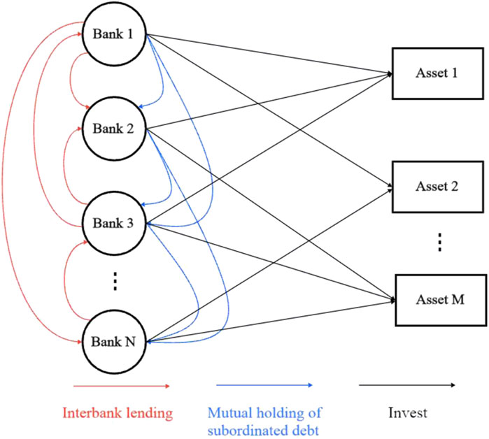
Figure 1. Interbank market structure.

In the actual banking system, banks usually hold subordinated debt with each other as a long-term capital replenishment mechanism to meet capital adequacy requirements. Subordinated debt can be traded in the secondary market, while interbank lending is mainly used to meet the short-term funding needs of banks and serves to manage liquidity, and is generally not transferred. In addition, the interrelation of interbank investment assets plays a critical part in the banking system’s stability. Multiple banks may invest in the same asset, and once one bank goes bankrupt and conducts an asset liquidation, the price of the asset will fluctuate, affecting the other banks holding the asset. In addition to causing asset price volatility, the failure of a bank may result in the bank’s inability to meet its loan and subordinated debt obligations, causing losses to the assets of creditor banks. In severe cases, it may even trigger a domino effect of consecutive bank failures. Insufficient liquidity of banks, which is closely correlated with factors such as investment, savings and lending, is the major factor of instability in the banking system. This article will use the model to analyze how these factors affect systemic risks in the banking system.

2.2 Model construction of multi-channel risk transmission among entities holding subordinated debt

In the actual banking system, the relationships between banks are complex and intertwined, involving not only direct relationships arising from interbank lending and holding subordinated debt, but also indirect relationships arising from joint investments in certain assets. In a random banking network, the interbank lending and the issuance and holding of subordinated debt are a process of random allocation. When banks have insufficient liquidity, they can borrow from other banks, with the link matrix represented by $J$, where $J_{ij}$ takes a value of 0 or 1. $J_{ij}=1$ indicates a possible lending relationship between bank $i$ and bank $j$, while $J_{ij}=0$ indicates no credit relationship between bank $i$ and bank $j$. $S$ represents the interconnection matrix of banks holding subordinated debt mutually, where when $S_{ij}$ > 0, the quantity of subordinated debt that bank $i$ holds in bank $j$ is $S_{ij}$, and when $S_{ij}$ < 0, the quantity of subordinated debt that bank $j$ holds in bank $i$ is $S_{ij}$, thus $S_{ij}=-S_{ij}$. The connection probability between banks is represented by $P$, where $0\le P_{ij}\le 1$.

Under the random banking network scenario, it is assumed that at time $t$, there exist $N_t$ banks, where $N_t$ is a bounded integer. As the discrete time evolves through $t=$ 1, 2, 3, … ,T, these $N_t$ banks form direct and indirect connections. At time $t$, bank $i$'s liquidity $L_i\left(t\right)$ is given by Equation 1:

${\mathit{L}}_{\mathit{i}}\left(\mathit{t}\right)=\overline{{\mathit{L}}_{\mathit{i}}}\left(\mathit{t}\right)-{\mathit{D}}_{\mathit{i}}\left(\mathit{t}\right)-{\mathit{I}}_{\mathit{i}}\left(\mathit{t}\right)+{\displaystyle \sum _{\mathit{j}=\mathbf{1}}^{{\mathit{N}}_{\mathit{t}}}}{\mathit{c}}_{\mathit{i}\mathit{j}}\left(\mathit{t}\right){\mathit{B}}_{\mathit{i}\mathit{j}}\left(\mathit{t}\right)(1)$

where $\overline{L_i}\left(t\right)$ is the liquid assets of bank $i$ that have not been invested, distributed and dismantled at time $t$; $D_i\left(t\right)$ is the distribution of dividends of bank $i$ at time $t$; $I_i\left(t\right)$ is the investment of bank $i$ at time $t$; $c_{ij}\left(t\right)$ represents the interbank loan association of bank $i$ with bank $j$ at time $t$. When there is a loan association of bank $i$ with bank $j$ at time $t$, $c_{ij}=1$, otherwise $c_{ij}=0$; $B_{ij}\left(t\right)$ refers to the loan volume between bank $i$ and bank $j$. When $B_{ij}\left(t\right)>0$, bank $i$ borrows money from bank $j$, and vice versa, bank $i$ lends money to bank $j$. In stochastic banking networks, borrowing only occurs when banks are illiquid, which is consistent with how banks actually operate.

At each time, the bank will carry out savings, dividends and investment operations, these operations will make the bank’s liquidity to alter, at time $t$, the bank’s liquidity without investment, dividends and savings $\overline{L_i}\left(t\right)$ can be expressed by Equation 2:

$\overline{{\mathit{L}}_{\mathit{i}}}\left(\mathit{t}\right)={\mathit{L}}_{\mathit{i}}\left(\mathit{t}-\mathbf{1}\right)+{\mathit{A}}_{\mathit{i}}\left(\mathit{t}\right)-{\mathit{A}}_{\mathit{i}}\left(\mathit{t}-\mathbf{1}\right)-{\mathit{r}}_{\mathit{a}}{\mathit{A}}_{\mathit{i}}\left(\mathit{t}-\mathbf{1}\right)+{\mathit{U}}_{\mathit{i}}\left(\mathit{t}\right)(2)$

where $r_a$ is the bank deposit interest rate, $A_i\left(t\right)$ represents the amount of deposit owned by bank $i$ at time $t$, and its concrete expression is $A_i\left(t\right)=\left(1+{\sigma }_A{\eta }_t\right)\overline{A}$, where ${\sigma }_A$ is the standard deviation of the total bank deposits, $\overline{A}$ is the average value of total bank deposits, ${\eta }_t\in N\left(0,1\right).U_i\left(t\right)$ denotes the investment profit earned in bank $i$ at time $t$, which is closely related to the total investment amount of bank $i$ at time $t$. Under the condition that bank $i$ has not invested at time $t$, the total investment amount of bank $i$ is expressed by Equation 3:

${\mathit{Y}}_{\mathit{i}}\left(\mathit{t}\right)={\displaystyle \sum _{\mathit{j}=\mathbf{1}}^{\mathit{M}}}{\mathit{Q}}_{\mathit{i}\mathit{j}}\left(\mathit{t}-\mathbf{1}\right){\mathit{g}}_{\mathit{j}}\left(\mathit{t}\right)(3)$

where $Q_{ij}\left(t-1\right)$ is the amount of equity in asset $j$ that bank i holds at time $t-1$, which is a dynamic value that reflects the realization of past investments and the development of new investments by bank $i$. $g_j\left(t\right)$ is the value of asset $j$ at time $t$, and its expression is given by Equation 4:

${\mathit{g}}_{\mathit{j}}\left(\mathit{t}\right)={\mathit{g}}_{\mathit{j}}\left(\mathit{t}-\mathbf{1}\right)\left(\mathbf{1}+{\mathit{\delta }}_{\mathit{j}}\left(\mathit{t}\right)\right)(4)$

where ${\delta }_j\left(t\right)$ is the yield of asset $j$ at time $t$, and it is not a fixed value, but a dynamic value influenced by many factors such as macroeconomics and policies. In this paper, ${\delta }_j\left(t\right)$ obeys a normal distribution with mean $\tau$, i.e., ${\delta }_j\left(t\right)\in N\left(\tau ,\theta \right)$. Where $\tau$ is the mean yield of all investments and $\theta$ is the asset value volatility.

When the bank’s liquidity is inadequate, it will choose to liquidate some assets to make up for the liquidity. At time $t$, the quantity of assets realized by bank $i$ is $U_i\left(t\right)=q\times Y_i\left(t\right)$, where $q$ is the ratio of realized investment. The aggregate investment assets owned by bank $i$ after the investment is realized and before continuing the investment are $\overline{Y_i}\left(t\right)={\displaystyle {\sum }_{j=1}^M}\overline{Q_{ij}}\left(t\right)g_j\left(t\right)$, where $\overline{Q_{ij}}\left(t\right)$ is the amount of shares in asset $j$ owned by bank $i$ following the realization of the partial investment. So the bank owner’s equity before dividends and investments can be expressed as Equation 5:

$\overline{{\mathit{V}}_{\mathit{i}}}\left(\mathit{t}\right)=\overline{{\mathit{L}}_{\mathit{i}}}\left(\mathit{t}\right)+\overline{{\mathit{Y}}_{\mathit{i}}}\left(\mathit{t}\right)-{\mathit{A}}_{\mathit{i}}\left(\mathit{t}\right)-\left(\mathbf{1}-{\mathit{r}}_{\mathit{b}}\right){\mathit{B}}_{\mathit{i}}\left(\mathit{t}-\mathbf{1}\right)(5)$

where $B_i\left(t-1\right)={\displaystyle {\sum }_{j=1}^{N_{t-1}}}{B}_{ij}\left(t-1\right)$ is the aggregate interbank debt owned by bank $i$ at time $t-1$, $r_b$ is the interbank offered rate. $\left(1+r_b\right)B_i\left(t-1\right)$ denotes the sum of the interbank borrowing capital and interest that bank $i$ has to repay at time $t$. When the bank generates investment income, it can pay dividends. The dividend of bank $i$ at time $t$ is determined by Equation 6:

${\mathit{D}}_{\mathit{i}}\left(\mathit{t}\right)=\mathit{max}\left\{\mathbf{0},\mathit{min}\left[{\mathit{U}}_{\mathit{i}}\left(\mathit{t}\right)-{\mathit{r}}_{\mathit{a}}{\mathit{A}}_{\mathit{i}}\left(\mathit{t}-\mathbf{1}\right),\overline{{\mathit{L}}_{\mathit{i}}}\left(\mathit{t}\right)-\mathit{\beta }{\mathit{A}}_{\mathit{i}}\left(\mathit{t}\right),\overline{{\mathit{L}}_{\mathit{i}}}\left(\mathit{t}\right)+\overline{{\mathit{Y}}_{\mathit{i}}}\left(\mathit{t}\right)-\left(\mathbf{1}+\mathit{\chi }\right){\mathit{A}}_{\mathit{i}}\left(\mathit{t}\right)\right]\right\}(6)$

where $\beta$ is the deposit reserve ratio and $\chi$ is the capital saving ratio. Dividend distribution by banks should be based on three premises: $\overline{V_i}\left(t\right)/A_i\left(t\right)\ge \chi$, net yield greater than 0, and meeting the requirements of deposit reserve. After paying dividends, the bank needs to reinvest the residual cash to obtain more returns. The investment made by bank $i$ at time $t$ is expressed as Equation 7:

${\mathit{I}}_{\mathit{i}}\left(\mathit{t}\right)=\mathit{min}\left\{\mathit{max}\left[\mathbf{0},\overline{{\mathit{L}}_{\mathit{i}}}\left(\mathit{t}\right)-\mathit{\beta }{\mathit{A}}_{\mathit{i}}\left(\mathit{t}\right)-{\mathit{D}}_{\mathit{i}}\left(\mathit{t}\right)\right],{\mathit{\omega }}_{\mathit{i}}\left(\mathit{t}\right)\right\}(7)$

where ${\omega }_i\left(t\right)=\overline{\omega }\left(1+{\sigma }_{\omega }\mu \right)$ is the investment opportunity of bank $i$ at time $t$, where $\overline{\omega }$ Is the average of all bank investment opportunities, ${\sigma }_{\omega }$ is the standard deviation of all bank investment opportunities, and $\mu$ obeys a normal distribution of $N\left(0,1\right)$. At time $t$, the amount of asset $j$ invested by bank $i$ is $∆Q_{ij}\left(t\right)$, which satisfies $I_i\left(t\right)={\displaystyle {\sum }_{j=1}^M}∆Q_{ij}\left(t\right){\mathrm{g}}_j\left(t\right)$. After investment $Y_i\left(t\right)$ satisfies the formula $Y_i\left(t\right)={\displaystyle {\sum }_{j=1}^M}{Q}_{ij}\left(t\right){\mathrm{g}}_j\left(t\right)$, where $Q_{ij}\left(t\right)=\overline{Q_{\text{ij}}}\left(t\right)+∆Q_{ij}\left(t\right)$.

2.3 Multichannel risk contagion model analysis of mutual subordinated debt holdings based on risk appetite

Within the framework of the banking system’s network, if a bank holds liquid funds after completing its dividend distribution and investment activities, it is considered to be a potential lender of funds, capable of providing financing support to other banks. When a bank is illiquid, it will need to incorporate funds from the interbank market to continue operating as usual. In case of the indebted bank, when the funds received from other banks are able to cover the preceding debt, the repayment operation will be carried out, and at the same time, the liquidity of this bank will be reduced to nil. If the bank is unable to raise sufficient funds to repay its debts and interest on deposits, it will have to dispose of its assets until the funds from the sale of assets can cover its debts. If the bank is unable to pay its debts after selling its assets, it will face bankruptcy and start the process of liquidation of assets. The proceeds of the liquidation will be applied first to pay off deposits and the remainder will be repaid to creditor banks on a pro rata basis.

During the process of issuing subordinated debt, the interest rate $r_i$ of subordinated debt of bank $i$ is determined by the ratio of bank $i$'s ownership interest to the average ownership interest of all banks. Its pricing follows the risk-return matching principle: banks with low capital adequacy ratios need to pay higher risk premiums to compensate investors. According to the Merton theory model, when equity declines, the risk of default increases exponentially, so the specific expression is as Equation 8:

$\mathit{f}\left({\mathit{r}}_{\mathit{i}}\right)=\overline{\mathit{r}}+\frac{{\mathit{e}}^{\mathbf{1}-\frac{{\mathit{V}}_{\mathit{i}}}{\overline{\mathit{V}}}}-\mathbf{1}}{\mathbf{1000}}(8)$

where $\overline{r}$ is the average subordinated interest rate of all banks, $V_i$ is bank $i$'s ownership interest, $\overline{V}$ is the average ownership interest of all banks. In the actual financial market, the interest rate at which a bank issues subordinated debt is affected by its own financial position. In assessing the credit rating of banks’ subordinated debt, credit rating agencies will take the banks’ financial indicators such as owner’s equity and capital adequacy ratio as important references. Usually, the subordinated debt issued by banks with better financial conditions can obtain a higher credit rating, thus attracting investors with lower interest rates. This is consistent with the model’s assumption that subordinated debt rates are negatively correlated with bank ownership equity. In the allocation process of subordinated debt, Bank i’s risk preference parameter is ρ, reflecting the bank’s level of risk preference. In the actual banking system, a bank’s risk preference is influenced by a variety of factors and cannot be fully captured by simple deterministic rules. Therefore, in this paper, the risk preference parameter is a random number between 0 and 1. The larger the risk preference parameter of banks, the more they like risk, and they tend to hold subordinated debt with higher interest rate; otherwise, they are more risk-averse and tend to hold subordinated debt with lower interest rate.

In the dynamic development of the banking system, selling assets tends to cause asset prices to fall. Since a number of financial intermediaries invest in the same asset at the simultaneous time, financial intermediaries are indirectly connected to each other through the assets in which they invest. Movements in asset prices can influence multiple institutions holding the asset at the same time, and changes in the assets of one financial institution can have an effect on other financial institutions through the assets jointly held. When banks are illiquid and unable to access loans, they sell assets to cover the liquidity gap. Furthermore, when a bank fails, the failing bank will liquidate its portfolio of assets, and the assets sold will decline in value. Banks holding the identical assets will be hit by the devaluation of their assets, leading to a loss of equity, which in turn may lead to insolvency, triggering bank bankruptcy, which can further damage the assets of creditor banks. Through this evolutionary process, the initial shock of the interbank network continues to propagate through the system. When a bank sells an asset due to illiquidity, or a bank goes into liquidation due to bankruptcy, the asset is sold at a depreciated value. Here, a market effect function is modeled through the price impact function in Equation 9:

$\mathit{f}\left({\mathit{x}}_{\mathit{j}}^{\mathit{t}}\right)={\mathit{e}}^{-\mathit{\alpha }{\mathit{x}}_{\mathit{j}}^{\mathit{t}}}(9)$

where $x_j^t$ is the liquidation portion of asset $j$ at time $t$. $\alpha$ represents the asset price sensitivity, i.e., the degree of price fluctuation resulting from the sale of the asset. In this paper, we take the value of $\alpha$ as 1.0536 in reference to the study of Caccioli [30], which indicates that when 10% of the assets are sold, the price of the assets will also fall by 10%, which can be approximated as the linear effect of asset sales on asset prices. Thus, the value of asset $j$ at time $t$ is as shown in Equation 10:

${\mathit{g}}_{\mathit{j}}\left(\mathit{t}\right)={\mathit{g}}_{\mathit{j}}\left(\mathit{t}\right)\mathit{f}\left({\mathit{x}}_{\mathit{j}}^{\mathit{t}}\right)(10)$

3 Model analysis

In the banking system evolutionary process, banks receive various ownership interests, liquid assets, dividends, etc., depending on their business conditions and strategies, and some banks go bankrupt due to poor business strategies. Due to systemic risk, the failure of one or a few banks may trigger a domino effect of more consecutive bank failures. In order to more clearly characterize systemic risk, we define systemic risk as in Equation 11:

$\mathit{R}\mathit{i}\mathit{s}\mathit{k}\left(\mathit{t}\right)=\frac{\mathbf{1}}{{\mathit{T}}_{\mathit{S}}{\mathit{N}}_{\mathit{e}}}{\displaystyle \sum _{\mathit{i}=\mathbf{1}}^{{\mathit{N}}_{\mathit{e}}}}{\displaystyle \sum _{\mathit{j}=\mathit{t}+\mathbf{1}}^{\mathit{t}+\mathit{T}}}\frac{{\mathit{M}}_{\mathit{j}}^{\mathit{i}}}{{\mathit{N}}_{\mathit{j}}^{\mathit{i}}}(11)$

where $T_S$ is the degree of time, $T_S=200$ in this paper, $N_e$ is the count of simulation repetitions, $N_j^i$ is the count of banks that are not insolvent at moment $j$, $M_j^i$ is the count of insolvent banks at the $i$ th simulation.

In this paper, the largest simulation time step is 2000, 200 banks are used in the simulation, and the simulation is performed 10 times, which can adequately represent the dynamic features of the banking system. At each time step, the bank can randomly recover 35% of its assets. There are 150 assets in which the bank can invest. The initial equity capital of the owner follows a normal curve with a mean of 200. The deposit interest rate is less than the investment return rate, i.e., $r_a<\delta$, which guarantees that the banking system will make a return. The larger the profit rate, the more profit the bank will receive, and the more stable the bank will be.

Figure 2 shows the change in the amount of banks in the banking system and the associated systemic risk, and the parameter is set to $r_a=0.004$, $r_b=0.008$, $\chi =0.3$, $\beta =0.25$, $\overline{A}=1000$, $\overline{\omega }=500$, ${\sigma }_a=0.15$, ${\sigma }_{\omega }=0.25$, $C=0.03$, $p=0.05$, $\tau =0.008$, $\theta =0.02$, $\overline{r}=0.008$. The trend in the amount of surviving banks over time in Figure 2 shows that in the early stages of the simulation, due to the interdependence of interbank assets and liabilities, the systemic risk was higher, leading to the rapid failure of some banks and a steep decrease in the amount of surviving banks. At the same time, systemic risk simulations decline rapidly at the initial stage, due to the fact that the initial situation of banks in the banking system is different, and the investment strategies developed are also different, and the systemic risk is greatest at this point. As it evolved, the banking system began to adapt and absorb some systemic risks, and gradually stabilized. In the realm of real finance, investment behavior itself contains risks. For banks with small and illiquid net worth, it is easy to fall into bankruptcy due to poor investment strategies. Failed banks may be incapable of repaying interbank loans in full, and overlapping bank portfolios can cause the value of other banks’ assets to shrink, triggering a domino effect of bank failures. For some banks in good initial condition, if the investment has a poor strategy and yield is low, it may eventually lead to a continuous decline in profits and bankruptcy.

Figure 2

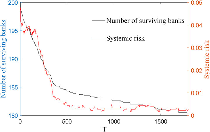
Figure 2. Evolution of the number of banks and systemic risks in the banking system.

Figure 3 shows the evolution process of various parameters of a bank based on the risk contagion model constructed in this article. The parameter settings are consistent with Figure 2. As shown in the figure, the parameters of the bank’s ownership equity, investment, dividends and liquidity change with the changes of internal and external factors in the banking system, and are in a state of dynamic change. When the ownership equity of the bank is greater than 0, the bank’s investment and dividends begin to increase, which is consistent with the actual operation of the bank.

Figure 3

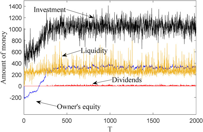
Figure 3. The evolution of the bank’s internal parameters.

This paper will further validate the validity of the model by analyzing the impact of parameters such as savings interest rate, savings volatility, reserve ratio, interbank lending rate, investment yield and volatility on systemic risk.

3.1 The impact of savings-related factors on systemic risk

Savings are essential for banks, not only as they are the main source of funding for banks, but also provide liquidity support to banks and are the basis for banks to make loans and other investment activities. Banks increase the value of their funds by paying interest on their savings to attract deposits, which are then used to make loans. The level of savings interest rate directly affects the bank’s cost of funds, which in turn affects the bank’s profitability and risk management.

Figure 4a illustrates the development of banks’ systemic risk under different savings interest rate conditions. The parameter settings are consistent with Figure 2 except for $r_a$. As the figure shows, the savings interest rate has a significant impact on the systemic risk of banks; the lower the savings interest rate, the more stable the banking system, and the systemic risk of banks increases as the savings interest rate rises. When the savings interest rate is higher, the bank needs to pay more interest, which will raise the bank’s funding cost, decrease the bank’s profit margin, and thus increase the bank’s operational risk. In addition, high interest rates can lead to the loss of deposits, further exacerbating banks’ liquidity risks and ultimately leading to the failure of some banks that are not in good shape.

Figure 4

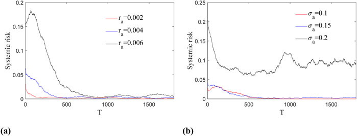
Figure 4. Evolution of systemic risk under different savings-related parameters: (a) Evolution of systemic risk under different savings rates; (b) Evolution of systemic risk under different savings volatility.

Figure 4b illustrates the evolution of systemic risk under different savings volatility conditions. The parameter settings are consistent with Figure 2 except for ${\sigma }_a$. It can be observed that when savings volatility is 0.1 and 0.15, the banking system eventually reaches a steady condition. When the savings volatility is 0.2, systemic risk is always at a high level. In reality, an increase in savings volatility means that banks face less deposit stability, which can lead to maturity matching issues for banks’ balance sheets. When market interest rates fluctuate greatly, depositors are more inclined to transfer funds to other investment products with higher returns, thus affecting the structure of banks’ funding sources. This flow of funds not only affects the liquidity of the bank, but can also result in a mismatch between the maturity of the assets and liabilities, increasing the bank’s liquidity risk and interest rate risk.

3.2 The impact of the reserve requirement ratio on systemic risk

The reserve requirement ratio is the lowest ratio of reserves that the central bank demands to be held by commercial banks and is main tools of monetary policy. In the early days of the statutory reserve system, its main function was risk management. By setting a statutory reserve ratio, the central bank mandates that commercial banks retain a fixed percentage of cash reserves to meet the withdrawal needs of depositors. This system has effectively reduced the incidence of bank runs and preserved the banking system’s stability [31]. Typically, a higher reserve requirement ratio (RRR) can enhance a bank’s resilience to risk, as a higher reserve deposit means that the bank has more funds to deal with possible depositor withdrawals and liquidity pressures, reducing the likelihood of a run on the bank.

Figure 5 shows the evolution of systemic risk in various RRR states. The parameter settings are consistent with Figure 2 except for $\beta$. The simulation result shows that either too high or too low a reserve ratio increases the systemic risk of banks. It is clear from the figure that before 500 time-steps, the systemic risk increases as the RRR increases. On the one hand, higher reserve ratios require banks to keep more funds as reserves to cover depositor withdrawals and short-term liquidity needs. This enhances banks’ ability to respond to runs and liquidity crises and reduces liquidity risk. On the other hand, excessively high reserve ratios reduce the funds available to banks for investment and lending, lowering investment income and interest income from loans, which in turn compresses profit margins and weakens banks’ profitability and competitiveness. Under such circumstances, banks may adopt more risky investment strategies to make up for lost profits, increasing their own risk exposure, which may be transmitted to other banks through the financial network, exacerbating systemic risk. After 500 steps, the systemic risk at $\beta =0.15$ exceeds the systemic risk at $\beta =0.25$, because when the reserve ratio is too small, the bank’s funds for investment increase, and the investment is risky, once the bank suffers a large loss, it is easy to go bankrupt. Therefore, policymakers need to consider when adjusting RRRs, and the need for further research on the specific effects of RRRs on systemic risk in different economic environments, so as to find a balance between enhancing bank stability and promoting economic growth.

Figure 5

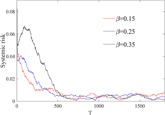
Figure 5. Evolution of systemic risk under different reserve ratios.

3.3 The impact of interbank lending rates on systemic risk

The lending rate is a major factor influencing the liquidity and stability of banks. In financial markets, banks manage their short-term funding needs through lending markets to ensure they can meet customer withdrawal needs and other short-term obligations. Figure 6 shows the evolution of banks’ systemic risk at different lending rates. The parameter settings are consistent with Figure 2 except for $r_b$. From the figure, it is obvious that with the increase of lending rates, bank systemic risk seems to have little change, that is, lending rate hardly affects the stable operation of the banking system. In June 2013, there was a turning point in China’s financial history, known as the “money shortage”. During this period, there was an extremely tight situation in the market, and all financial entities followed the principle of “cash is king” and refused to lend funds. On June 20, the Shanghai Interbank Offered Rate (SHIBOR) reached 13.44% [32], and the interbank market pledged repo rate (R001) hit a record high of 30%, but in the end, there was no bank bankruptcy, consistent with the simulation results. One reason was that the impact of short-term interbank lending rate shocks could be absorbed through investment returns, and the other was that the central bank injected 360 billion yuan in liquidity to prevent risk contagion. Similar cases include the 2008 financial crisis, when the United States 3-month LIBOR reached 4.82% but no large-scale bank failures occurred, and the 2011 European debt crisis, when the Euribor rose to 5.2% but core economies did not collapse. This indicates that, under an effective policy environment, the direct impact of interbank lending rates on systemic risk can be ignored. However, their sustained high levels may signal underlying pressures that require policy responses. The impact of investment-related parameters on systemic risk.

Figure 6

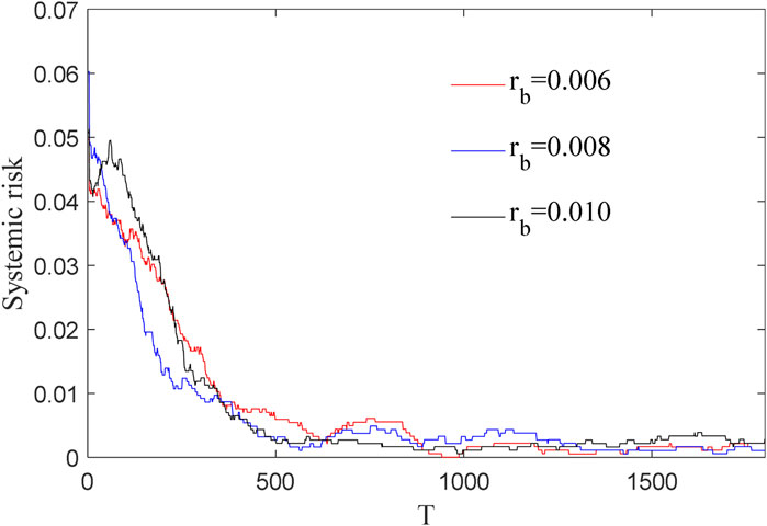
Figure 6. Evolution of systemic risk under different lending rates.

In the real financial market, the rate of return on investment is an important indicator to measure the profitability of a bank’s investment activities. It reflects the ratio between the income that a bank earns through its investment activities and the cost of its investment. A higher yield usually means that the bank’s investment activities are more successful, which can lead to a more stable source of income for the bank, thereby enhancing the bank’s profitability and stability. Conversely, a lower yield means that the bank’s investment activities are subject to higher risk, which may affect the stability of the bank.

Figure 7a shows the evolution of banks’ systemic risk under various average rates of return. The parameter settings are consistent with Figure 2 except for $\tau$. It is evident that the higher the average rate of return, the lower the banks’ systemic risk. Over the entire period, the systemic risk at $\tau =0.01$ decreases the fastest and is consistently lower than the systemic risk values at $\tau =0.008$ and $\tau =0.006$, and the banking system reaches stability at 500 steps, while the systematic risk is always maximum at $\tau =0.006$. This is due to the fact that when the return on investment is large, a large interest rate differential can be generated between investment profits and savings interest, which can improve the bank’s profitability and liquidity, thereby improving the bank’s ability to resist risks and reduce systemic risks.

Figure 7

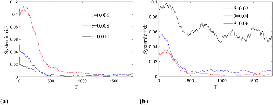
Figure 7. Evolution of systemic risk under different investment-related parameters: (a) Evolution of systemic risk under different average returns; (b) Evolution of systemic risk under different ROI fluctuations.

Figure 7b illustrates banks’ systemic risk under different ROI fluctuations. The parameter settings are consistent with Figure 2 except for $\theta$. It is clear that in the initial phase, the systemic risk measures were high for all curves, but over time, these indicators showed a downward trend. Throughout the time period, the systemic risk at ROI of 0.02 and 0.04 decreased rapidly, and the banking system was relatively stable, while the banking system was always exposed to higher systemic risk when the ROI was 0.06. This result shows that lower volatility of return on investment can help reduce the banking system’s systemic risk, because when the volatility of investment is low, the investment income of banks is more stable, and the possibility of excessive losses in investment activities is less, which means that banks can effectively control risks and the banking system is more stable. When the investment volatility is high, the bank is more likely to suffer investment losses, and if the bank is not in a good state at this time, it can easily lead to the bank’s bankruptcy.

3.4 The impact of bank size on systemic risk

In complex financial networks, bank size is not only a measure of the size of a single institution, but also a key hub for the propagation of systemic risk. In this paper, banks are categorized into different types according to their size, where those with an initial ownership interest of less than 100 are small-sized banks, those with an initial ownership interest between 100 and 500 are medium-sized banks, and those with an initial ownership interest greater than 500 are large-sized banks. The number of different types of banks and the percentage of failed banks are given in Table 1. From the table it can be seen that small scale banks have the highest number of failures followed by medium scale banks and large-scale banks have almost no failures. This phenomenon is consistent with the “too big to fail” hypothesis. In fact, large banks are highly systemically important due to their size and influence [33], and are unable to cope with the negative knock-on effects of failure, so they will tide over the difficulties with government support. 2008 financial crisis, Lehman Brothers, due to over-investment in financial derivatives related to subprime bonds in the real estate market bubble, has become a major player in the financial crisis. Subprime debt-related financial derivatives, and suffered huge losses when the real estate market collapsed, and eventually filed for bankruptcy protection on September 15, 2008. Therefore, despite the low rate of large-scale bank failures, cross-asset investments and subprime exposures need to be monitored. On the other hand, the likelihood of a financial crisis depends on the liquidity position of banks in the system [34], so small and medium-sized banks need improved liquidity support to reduce the likelihood of outright bankruptcy.

Table 1

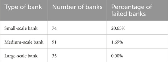
Table 1. Number of different types of banks and proportion of failed banks.

3.5 Impact of falling asset prices on systemic risk

In order to assess the robustness of the banking system to extreme shocks, this study designs an asset price crash scenario with reference to historical financial crisis characteristics. Figure 8 presents the evolutionary results of the banking network suffering a 40% fall in asset prices at step 750, with the same parameter settings as in Figure 2. From the figure, it can be seen that the number of insolvent banks increases rapidly after suffering an asset price fall, and due to the high degree of correlation in the banking system, the asset price fall transmits risk among banks through multiple channels, which leads to a domino effect of a large number of banks failing one after another.

Figure 8

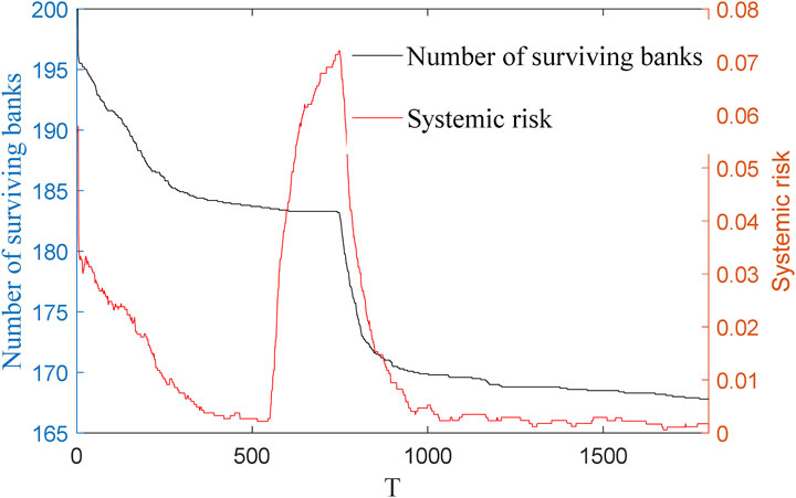
Figure 8. Evolutionary outcomes of bank networks when asset prices fall.

The results in Figure 8 show that systemic risk, after a short-term sharp rise, gradually decreases to a steady state, the number of bank failures gradually decreases, and the banking system stabilizes, indicating that the banking network is able to gradually absorb systemic risk.

On the basis of the foregoing analysis, it may be concluded that the banking system’s stability is related to a variety of factors. Table 2 demonstrates the impact of several key parameters on systemic risk, and here we analyze it in the context of the specific economic situation. When the economy is growing steadily, the banking system is generally exposed to low systemic risk. In this environment, investor yields are usually higher and less volatile, helping banks maintain stable profitability and thus enhancing their stability. In times of increased economic uncertainty or economic downturn, banks may be exposed to higher systemic risks, especially when the reserve requirement ratio is high, which may limit banks’ lending capacity and affect their profitability and liquidity. At this juncture, an appropriate reduction in the reserve requirement ratio and the savings interest rate is conducive to replenishing banks’ liquidity and improving their ability to withstand risks. Therefore, banks and policymakers need to pay close attention to changes in these factors and take appropriate risk control measures to preserve the banking system’s stability.

Table 2

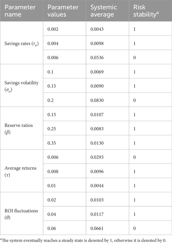
Table 2. The impact of key parameters on systemic risk.

4 Discussion

The financial system is a complicated network structure consisting of diversified financial entities and their interactions, which include not only the direct relationship between interbank loans and cross-ownership of subordinated debt, but also the indirect coupling effect caused by the convergence of asset allocation. It is of great significance for regulators and bank policymakers to study the impact of bank savings interest rates and their fluctuations, interbank lending rates, reserve requirement ratios, and investment yields and fluctuations on bank stability. Previous studies have mostly focused on the coupling of interbank lending and investment, and few have taken into account cross-subordinated debt holdings. In addition, it is difficult for the existing model to truly reflect the dynamic development of the banking system because some assumptions in the existing model are not realistic, such as the same interest rate on subordinated bonds issued by each bank, and the risk appetite of the bank is not taken into account. To better reflect the development of the banking system, this paper establishes a multichannel risk contagion model from the risk appetite perspective, which comprehensively considers interbank loans, investment coupling, and the holding of subprime bonds with different interest rates according to different risk appetite levels. Based on multi-dimensional simulation and theoretical deduction, this paper draws the following conclusions.

(1) The savings interest rate can directly affect the bank’s cost of funds, which in turn affects the profitability and stability of the bank. The higher the savings interest rate of the bank, the higher the fluctuations of savings and the higher the systemic risk. Appropriately lowering the interest rate on savings and reducing the fluctuation of savings is conducive to improving the stability of banks.

(2) A reserve requirement ratio that is too high or too low will raise the systemic risk of banks. If the reserve requirement ratio is too high, it will reduce the interest rate spread between investment and savings, and concurrently limit the bank’s lending ability, affect the bank’s profitability, and increase systemic risk. The smaller the interest rate on deposits, the more money the bank uses for investment, and the higher the bank’s risk.

(3) The interbank lending rate is not a significant factor in the systemic risk of banks.

(4) The higher the average return on investment, the more stable the bank will be. If the bank’s investment return is too low, the bank will not be able to make sufficient profits, which will have the effect of reducing liquidity and weakening the ability of the bank to resist risks. The less volatile the investments, the lower the bank’s systemic risk. A sound investment strategy is also essential to improve the stability of the bank.

Based on the above conclusions, we propose the following policy recommendations: For regulatory authorities, it is necessary to improve the monitoring indicator system for banking system stability, fully considering the impact of factors such as savings interest rates, reserve ratios, investment returns, and volatility on systemic risk, closely monitoring trends in these indicators, and promptly identifying potential risks. When formulating and adjusting reserve requirement ratio policies, the dual impact on systemic risks in the banking system should be carefully balanced. Differentiated reserve requirement ratio policies can be implemented based on the scale and risk characteristics of different types of banks. Additionally, an emergency mechanism for the interbank lending market should be established and improved, with enhanced monitoring of the flow of interbank lending funds. For banks themselves, savings products should be priced reasonably, with savings interest rates determined scientifically and reasonably based on their cost structures, risk preferences, and market competition conditions. Banks should also optimize their asset allocation strategies, focusing on diversification and balancing risk and return, while reasonably controlling the volatility of investment assets. Furthermore, banks should strengthen liquidity risk management, reasonably arrange funding sources and usage, ensure sufficient liquidity to address funding shortages, and enhance communication and coordination with the central bank and other financial institutions.

This study constructs a dynamic evolution model framework, which aims to quantitatively measure and analyze the mechanism of bank systemic risk in the context of macroeconomic cyclical fluctuations, and provides methodological support for regulators to identify risk contagion paths and formulate forward-looking prevention and control strategies. Future research directions can focus on the following aspects: first, calibrating model parameters based on real transaction data to improve the empirical adaptability of risk prediction; Second, more heterogeneous bank behavior assumptions (such as differentiated liquidity management strategies) are introduced to enhance the explanatory power of the model to the complex financial ecology. This will further improve the dynamic monitoring framework for systemic risks and provide a science-based foundation for the precise implementation of macroprudential policies.

Data availability statement

Publicly available datasets were analyzed in this study. This data can be found here: https://github.com/knochen336/Risk-Contagion-of-Banks-Holding-Subordinated-Debt/.

Author contributions

SC: Data curation, Writing – original draft, Methodology, Software. SJ: Project administration, Writing – review and editing, Conceptualization, Funding acquisition, Supervision. YZ: Investigation, Formal Analysis, Data curation, Writing – review and editing. LM: Writing – review and editing, Visualization, Investigation, Validation.

Funding

The author(s) declare that financial support was received for the research and/or publication of this article. This work is funded by Ministry of Education, Humanities and social science projects (21YJC790054) and National Natural Science Foundation of PR China (72101121).

Conflict of interest

The authors declare that the research was conducted in the absence of any commercial or financial relationships that could be construed as a potential conflict of interest.

Generative AI statement

The author(s) declare that no Generative AI was used in the creation of this manuscript.

Publisher’s note

All claims expressed in this article are solely those of the authors and do not necessarily represent those of their affiliated organizations, or those of the publisher, the editors and the reviewers. Any product that may be evaluated in this article, or claim that may be made by its manufacturer, is not guaranteed or endorsed by the publisher.

References

1. Poledna S, Martínez-Jaramillo S, Caccioli F, Thurner S. Quantification of systemic risk from overlap portfolios in the financial system. J Financial Stab (2021) 52:100808. doi:10.1016/j.jfs.2020.100808

CrossRef Full Text | Google Scholar

2. Jackson MO, Pernoud A. Systemic risk in financial networks: a survey. Annu Rev Econ (2021) 13(1):171–202. doi:10.1146/annurev-economics-083120-111540

CrossRef Full Text | Google Scholar

3. Craig B, Ma Y. Intermediation in the interbank lending market. J Financial Econ (2022) 145(2):179–207. doi:10.1016/j.jfineco.2021.11.003

CrossRef Full Text | Google Scholar

4. Qi M, Shi D, Feng S, Wang P, Nnenna AB. Assessing the interconnectedness and systemic risk contagion in the Chinese banking network. Int J Emerging Markets (2022) 17(3):889–913. doi:10.1108/ijoem-08-2021-1331

CrossRef Full Text | Google Scholar

5. Liu X. Unraveling systemic risk transmission: an empirical exploration of network dynamics and market liquidity in the financial sector. J Knowledge Economy (2024) 16:6629–64. doi:10.1007/s13132-024-01861-9

CrossRef Full Text | Google Scholar

6. Macchiati V, Brandi G, Di Matteo T, Paolotti D, Caldarelli G, Cimini G. Systemic liquidity contagion in the European interbank market. J Econ Interaction Coord (2022) 17(2):443–74. doi:10.1007/s11403-021-00338-1

CrossRef Full Text | Google Scholar

7. Yanquen E, Livan G, Montañez-Enriquez R, Martinez-Jaramillo S. Measuring systemic risk for bank credit networks: a multilayer approach. Latin Am J Cent Banking (2022) 3(2):100049. doi:10.1016/j.latcb.2022.100049

CrossRef Full Text | Google Scholar

8. Capponi A, Sun X, Yao DD. A dynamic network model of interbank Lending—Systemic risk and liquidity provisioning. Math Operations Res (2020) 45(3):1127–52. doi:10.1287/moor.2019.1025

CrossRef Full Text | Google Scholar

9. Gao Q, Lv D, Jin X. Systemic risk of multi-layer financial network system under macroeconomic fluctuations. Front Phys (2022) 10:943520. doi:10.3389/fphy.2022.943520

CrossRef Full Text | Google Scholar

10. Ding Z, Yan H, Chen Y, Jiang C. Risk contagion in interbank lending networks: a multi-agent-based modeling and simulation perspective. Expert Syst Appl (2024) 256:124847. doi:10.1016/j.eswa.2024.124847

CrossRef Full Text | Google Scholar

11. Fan H, Sheng W. Research on dynamic evolution of systemic risk in Chinese banking system. Front Phys (2020) 8:199. doi:10.3389/fphy.2020.00199

CrossRef Full Text | Google Scholar

12. Zou J, Fu X, Yang J, Gong C. Measuring bank systemic risk in China: a network model analysis. Systems (2022) 10(1):14. doi:10.3390/systems10010014

CrossRef Full Text | Google Scholar

13. Jin S, Song L, Shu L, Gao Q, Chen Y. Systemic risk in Chinese interbank lending networks: insights from short-term and long-term lending data. Empirical Econ (2024) 67:2539–64. doi:10.1007/s00181-024-02617-9

CrossRef Full Text | Google Scholar

14. Krause A, Giansante S. Interbank lending and the spread of bank failures: a network model of systemic risk. J Econ Behav and Organ (2012) 83(3):583–608. doi:10.1016/j.jebo.2012.05.015

CrossRef Full Text | Google Scholar

15. Li S, Liu M, Wang L, Yang K. Bank multiplex networks and systemic risk. Physica A: Stat Mech Its Appl (2019) 533:122039. doi:10.1016/j.physa.2019.122039

CrossRef Full Text | Google Scholar

16. Wang H, Li S. Optimization of systemic risk: reallocation of assets based on bank networks. J Risk (2021). doi:10.21314/JOR.2020.449

CrossRef Full Text | Google Scholar

17. Huang Y, Liu T. Diversification and systemic risk of networks holding common assets. Comput Econ (2023) 61(1):341–88. doi:10.1007/s10614-021-10211-9

CrossRef Full Text | Google Scholar

18. Ma J, He J, Liu X, Wang C. Diversification and systemic risk in the banking system. Chaos, Solitons and Fractals (2019) 123:413–21. doi:10.1016/j.chaos.2019.03.040

CrossRef Full Text | Google Scholar

19. Zou L, Xie L, Yang Y. A double-layer network and the contagion mechanism of China's financial systemic risk. J Artif Societies Soc Simulation (2019) 22(4). doi:10.18564/jasss.4122

CrossRef Full Text | Google Scholar

20. Gao Q, Fan H. Systemic risk caused by the overlapping portfolios of banks under a bilateral network. Front Phys (2021) 9:638991. doi:10.3389/fphy.2021.638991

CrossRef Full Text | Google Scholar

21. Caccioli F, Barucca P, Kobayashi T. Network models of financial systemic risk: a review. J Comput Soc Sci (2018) 1:81–114. doi:10.1007/s42001-017-0008-3

CrossRef Full Text | Google Scholar

22. Nguyen T. The disciplinary effect of subordinated debt on bank risk taking. J empirical Finance (2013) 23:117–41. doi:10.1016/j.jempfin.2013.05.005

CrossRef Full Text | Google Scholar

23. Capponi A, Weber M. Systemic portfolio diversification. Operations Res (2024) 72(1):110–31. doi:10.1287/opre.2022.0290

CrossRef Full Text | Google Scholar

24. Shen P, Li Z. Financial contagion in inter-bank networks with overlapping portfolios. J Econ Interaction Coord (2020) 15(4):845–65. doi:10.1007/s11403-019-00274-1

CrossRef Full Text | Google Scholar

25. Weber S, Weske K. The joint impact of bankruptcy costs, fire sales and cross-holdings on systemic risk in financial networks. Probab Uncertainty Quantitative Risk (2017) 2:9–38. doi:10.1186/s41546-017-0020-9

CrossRef Full Text | Google Scholar

26. Wang C, Liu X, He J. Does diversification promote systemic risk? North Am J Econ Finance (2022) 61:101680. doi:10.1016/j.najef.2022.101680

CrossRef Full Text | Google Scholar

27. Jiang S, Fan H. Systemic risk in the interbank market with overlapping portfolios and cross-ownership of the subordinated debts. Physica A: Stat Mech its Appl (2021) 562:125355. doi:10.1016/j.physa.2020.125355

CrossRef Full Text | Google Scholar

28. Yan C, Ding Y, Liu W, Liu X, Liu J. Multilayer interbank networks and systemic risk propagation: evidence from China. Physica A: Stat Mech its Appl (2023) 628:129144. doi:10.1016/j.physa.2023.129144

CrossRef Full Text | Google Scholar

29. Fan H, Pan H. The effect of shadow banking on the systemic risk in a dynamic complex interbank network system. Complexity (2020) 2020(1):1–10. doi:10.1155/2020/3951892

CrossRef Full Text | Google Scholar

30. Caccioli F, Shrestha M, Moore C, Farmer JD. Stability analysis of financial contagion due to overlapping portfolios. J Banking and Finance (2014) 46:233–45. doi:10.1016/j.jbankfin.2014.05.021

CrossRef Full Text | Google Scholar

31. Pan H, Fan H. The stability of banking system with shadow banking on different interbank network structures. Discrete Dyn Nat Soc (2021) 2021(1):1–15. doi:10.1155/2021/6650327

CrossRef Full Text | Google Scholar

32. Chen B, Li L, Peng F, Anwar S. Risk contagion in the banking network: new evidence from China. North Am J Econ Finance (2020) 54:101276. doi:10.1016/j.najef.2020.101276

CrossRef Full Text | Google Scholar

33. Zhang X, Zhang X, Lee CC, Zhao Y. Measurement and prediction of systemic risk in China’s banking industry. Res Int Business Finance (2023) 64:101874. doi:10.1016/j.ribaf.2022.101874

CrossRef Full Text | Google Scholar

34. Chen H, Wang T, Yao DD. Financial network and systemic Risk—A dynamic model. Prod Operations Manag (2021) 30(8):2441–66. doi:10.1111/poms.13384

CrossRef Full Text | Google Scholar