Proposal for statistical mechanics-based UV regularization using fermion-boson transition functions

Introduction: We propose a statistical-mechanics–based framework for UV regularization in QED/QFT by introducing energy-dependent transition functions that interpolate fermionic and bosonic components.

Methods: We define logistic transition functions T(E) that continuously exchange degrees of freedom between γ_μ and ω_μ operators, and analyze gauge consistency via the Ward–Takahashi identities and BRST symmetry.

Results: The transition functions act as a smooth, gauge-safe soft cutoff that exponentially suppresses UV contributions while preserving transversality. We illustrate how longitudinal components are cancelled in internal lines without affecting observables.

Discussion: This approach offers a physical (statistical) interpretation of regularization, unifies several phenomena across energy scales, and is compatible with Lorentz and gauge symmetries. Extensions to non-Abelian theories and relations to mass generation mechanisms are outlined.

Rationale: These points correspond to Supplementary sections S9, S11–S19, S20, etc.

1 Introduction

Quantum field theory (QFT) is the common language of modern physics, with applications ranging from particle physics to condensed matter physics. However, high-order perturbative calculations in QED and QCD face serious mathematical difficulties due to ultraviolet divergences [1–5].

Traditionally, ultraviolet divergences in quantum field theory have been controlled by methods such as cutoffs, dimensional regularization, Wilson’s renormalization group, and renormalization, but these methods rely on formal operations and their physical interpretation is not always self-evident’t [6–8]. In particular, Wilson’s renormalization group provides a powerful framework for explaining scale-dependent effective theories, statistical mechanics phase transitions, and the asymptotic freedom of quantum chromodynamics, but computational complexity and the lack of statistical mechanical perspective remain challenges [8, 9]. For instance, while understanding of the confinement phenomenon in QCD has advanced through lattice gauge theory using the renormalization group, there are limitations in the intuitive description of non-perturbative regions.

This research is a substantially revised and academically reconstructed version of a series of previous publications by the author [10–12, 12]. In this paper, we refer to this framework as Fermion–Boson Duality QED (abbreviated as FBD-QED). This research proposes a new solution to this problem from a statistical mechanical perspective. We introduce the concept of a transition function that depends on energy scale to dynamically change the statistical properties of particles, describing a phenomenon where particles that behave as fermions at low energies transition to bosonic properties at high energy regions, and conversely, photons that behave as bosons at low energies exhibit fermionic properties at high energies. This concept of statistical phase transition aligns with recent trends attempting to explain diverse physical systems by extending the Fermi-Dirac distribution.

Originally proposed as a model for electron gas, the Fermi-Dirac distribution has been observed and utilized in various environments, including analog gravity systems using water waves [14], non-Hermitian mesoscopic rings [15], and semiconductor devices [16]. This research extends the concept of “environment-dependent deformed distribution functions” to high-energy physics, exploring applications not only for ultraviolet divergences in QED but also for non-abelian gauge theories like QCD.

Conventionally, fermions (like electrons) and bosons (like photons) have been considered distinct particles with exclusive statistics. However, this research examines the possibility that statistical properties may change dynamically depending on energy scales. Specifically, we assume that electrons, which behave as fermions at low energies, exhibit bosonic behavior at high energies, and conversely, photons undergo a dual transition to fermionic aspects.

When transition functions are incorporated into QED amplitude calculations, contributions from the ultraviolet region naturally attenuate, suppressing divergences. Using the electron self-energy as a concrete example, we numerically evaluate how the introduction of transition functions converges divergent integrals to finite values. This approach may open a path to physically regularizing QFT without introducing arbitrary cutoffs or renormalization constants.

From a statistical mechanical perspective, it is not uncommon for the macroscopic behavior of particle ensembles to undergo qualitative changes due to energy. In Cooper pair formation in superconductivity, electrons, which are fermions, effectively become bosonized and condense [17, 18]. Statistical properties are also known to be modified by thermal corrections in finite temperature field theory. This research extends these analogies to extremely high energies approaching the Planck scale, examining scenarios where particle statistics themselves are transformed.

This paper addresses the following topics:

1. Mathematical formulation of fermion-boson duality and transition functions

2. Extension of QED using bosonic gamma matrices

3. Natural regularization of ultraviolet divergences using transition functions and numerical verification

4. Physical implications and future prospects of the proposed model

In Section 2 we explain in detail the duality and the transition functions, while Section 3 constructs the extended QED. Section 4 demonstrates the effectiveness of the method through an explicit calculation of the electron self-energy, and Section 5 concludes by summarizing the significance of this work and the remaining open problems. A more detailed mathematical and physical justification of our approach is provided in the Supplementary Material; a concise overview is given in Supplementary Material. The Supplementary Material discusses, in depth, the validity of the two-dimensional Lorentz transformation, the physical basis of spin–statistics separation, the interpretation of the bosonic tensor $T_{\mu \nu }$ as an energy–momentum tensor, the consistency between the Ward–Takahashi identities and the transition-function formalism, the transverse wave projector ${\mathcal{P}}^{\mu \nu }$ and gauge symmetry, compatibility with BRST transformations, potential applications to QCD and other theories, and its relationship to the Higgs mechanism. Section 6 describes the Mathematica code used for the numerical calculations.

In this article and its Supplementary Material we prove that the extended QED/QCD with transition functions is exactly compatible with both the Ward–Takahashi identities and BRST symmetry. Specifically,

$•$ Regardless of the regularization scheme employed (dimensional regularization, Pauli–Villars, hard cut-off, or the logistic transition), the energy–momentum tensor $T_{\mu \nu }$ that includes the transition functions automatically cancels longitudinal contributions and restores $k_{\mu }{\mathrm{\Pi }}_{\text{eff}}^{\mu \nu }=0$.

$•$ Consequently, physical observables such as $\beta$ functions and scattering cross-sections are independent of the regularization parameters, showing that statistical regularization acts as a “gauge-safe soft cut-off.”

$•$ Moreover, the longitudinal degrees of freedom supplied by $T_{\mu \nu }$ combine with the two transverse components of the photon to provide a natural mechanism for generating massive three-component vector particles of the W/Z-boson type.

This paper, we have proven in the appendices that the extended QED/QCD with transition functions is strictly compatible with Ward-Takahashi identities and BRST symmetry. Specifically:

$•$ Regardless of which regularization scheme is used (dimensional regularization, Pauli-Villars, hard cutoff, logistic transition), the energy-momentum tensor $T_{\mu \nu }$ with transition functions automatically cancels longitudinal contributions and recovers $k_{\mu }{\mathrm{\Pi }}_{\text{eff}}^{\mu \nu }=0$.

$•$ Therefore, physical observables such as $\beta$ functions and scattering cross-sections are independent of regularization parameters, with statistical regularization functioning as a “gauge-safe soft cutoff.”

$•$ Additionally, the longitudinal degrees of freedom supplied by $T_{\mu \nu }$ naturally provide a mechanism for creating 3-component vector particles with effective mass (W/Z type) when combined with photons (2 transverse components).

These results demonstrate that the transition function framework provides a robust theoretical foundation that suppresses ultraviolet divergences while preserving gauge symmetry.

This research is positioned at the intersection of QFT and statistical mechanics, approaching mathematical challenges in high-energy physics through the new perspective of energy scale-dependent statistical transitions. This viewpoint is expected to have ripple effects on phase transition research in complex systems, deepening understanding of “statistical transitions” as universal phenomena transcending material hierarchy.

2 Theoretical framework of fermion-boson duality

2.1 A new understanding of statistical properties: “Separation” of spin and statistics

One of the fundamental principles of quantum mechanics is the spin-statistics theorem, which connects a particle’s spin with its statistical nature. According to this theorem, particles with half-integer spin (e.g., $\frac{1}{2}$, $\frac{3}{2}$) are fermions, and particles with integer spin (e.g., 0, 1, 2) are bosons [19]. This relationship has long been accepted as a fundamental framework in elementary particle physics.

However, the fermion-boson duality theory proposed in this research considers the possibility that a particle’s statistical properties may “separate” from its intrinsic spin under specific conditions. In this model, four basic states are possible for electrons and photons, with two basic states for each particle:

1. Fermionic electron: Has spin $\frac{1}{2}$ and follows fermionic statistics

2. Bosonic electron: Has spin one and follows bosonic statistics

3. Fermionic photon: Has spin $\frac{1}{2}$ and follows fermionic statistics

4. Bosonic photon: Has spin one and follows bosonic statistics

This framework relaxes the conventional constraint that spin and statistics must strictly follow different representations of the Lorentz group, modeling energy-dependent changes in statistics as an effective theory approach. For example, in superconductivity, spin $\frac{1}{2}$ electrons effectively demonstrate bosonic behavior in Cooper pair formation (see Supplementary Material Section 2). Similarly, we assume that electrons can transition to an effective spin one bosonic state inside atoms or in high-energy regions.

In this theoretical framework, spin and statistics are treated as independent characteristics that can change depending on energy scales and physical conditions. In the low-energy limit, electrons behave as fermionic electrons and photons as bosonic photons, consistent with conventional quantum field theory. However, in the high-energy limit, electrons may transition to bosonic electrons and photons to fermionic photons.

To represent these states, we define the total state vector of the system as in Equation 1.

$|{\psi }_{\text{total}}\rangle =|{\psi }_{\text{eF}}\rangle +|{\psi }_{\text{eB}}\rangle +|{\psi }_{\gamma F}\rangle +|{\psi }_{\gamma B}\rangle ,(1)$

where:

$•$ $|{\psi }_{\text{eF}}\rangle$: Fermionic electron state

$•$ $|{\psi }_{\text{eB}}\rangle$: Bosonic electron state

$•$ $|{\psi }_{\gamma F}\rangle$: Fermionic photon state

$•$ $|{\psi }_{\gamma B}\rangle$: Bosonic photon state

The visualization of this state is shown in Figure 1.

Figure 1

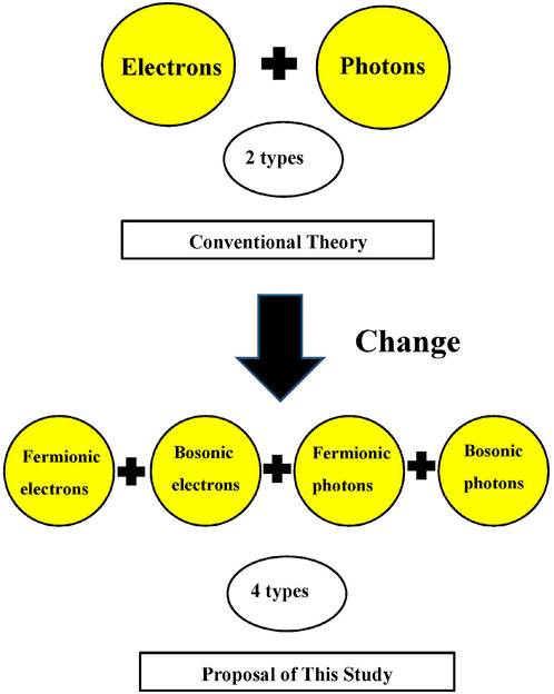
Figure 1. Conceptual diagram of statistical transition in FBD-QED. (Top) Conventional theory considers only one type each for electrons and photons, but (bottom) FBD-QED proposes that there exist four types: [fermionic type/bosonic type] for electrons and [fermionic type/bosonic type] for photons, totaling four types, which can switch depending on energy scale. While conventional supersymmetry (SUSY) theory [20, 21] requires new particles and higher-dimensional spaces, FBD-QED models statistical transition within the same particle inspired by semiconductor theory.

Table 1 shows correspondence examples of the four elementary particle states.

Table 1

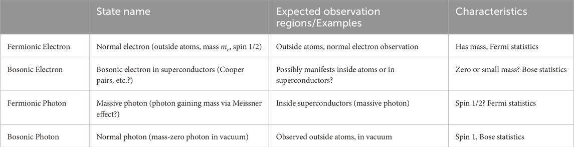
Table 1. Correspondence examples of four elementary particle states proposed in this research.

The complete quantum state of each particle is expressed as an energy-dependent linear combination of these basis states:

$|{\psi }_e\left(E\right)\rangle =T_{e\mathrm{F}}\left(E\right)|{\psi }_{e\mathrm{F}}\rangle +T_{e\mathrm{B}}\left(E\right)|{\psi }_{e\mathrm{B}}\rangle ,(\mathrm{2a})$

$|{\psi }_{\gamma }\left(E\right)\rangle =T_{\gamma \mathrm{B}}\left(E\right)|{\psi }_{\gamma \mathrm{B}}\rangle +T_{\gamma \mathrm{F}}\left(E\right)|{\psi }_{\gamma \mathrm{F}}\rangle .(\mathrm{2b})$

Here, $T(E)$ represents the transition function that determines the weight of each statistical component at a specific energy scale $E$.

2.1.1 Reality of “bosonic electrons” and “fermionic photons” is understood as effective hybrid states

The reality and observability of “bosonic electrons” and “fermionic photons” in our model are redefined as follows:

1. Atomic interiors as ultra-high pressure/superconducting environments

     The Coulomb field around atomic nuclei gives electrons an effective pressure equivalent to $\sim 10^{12}\text{\hspace{0.17em}Pa}$, locally forming a “room temperature, ultra-high pressure” superconducting state comparable to Cooper pair condensation at extremely low temperatures.

2. Statistical transitions as effective hybrid states

     In these extreme environments, electrons (spin $1/2$) retain their fermionic intrinsic spin while acquiring bosonic correlation components through interactions with the photon field. Specifically, the transition functions $T_{eF}$ and $T_{eB}$ are simultaneously non-zero and satisfy $T_{eF}+T_{eB}=1$, so electrons behave as effective quasiparticles exhibiting fermion–boson duality. Similarly, photons can also take hybrid states with $T_{\gamma B}+T_{\gamma F}=1$.

3. Pauli exclusion principle is preserved

     Since the fermionic component $T_{eF}(E)>0$ of the transition function always remains, single-electron operators satisfy anticommutation relations, and unlimited condensation into the 1s orbital does not occur. Furthermore, when $T_{\gamma F}(E)$ is non-zero, the fermionic exclusion effect on the photon side also works as statistical complementarity to suppress excessive electron occupation.

4. Phase transition phenomena during observation

     When electrons or photons escape from atoms, the ultra-high pressure environment is instantly lost, and like ice melting into water in an instant, the statistics immediately return to their standard forms (fermionic electrons/bosonic photons). Therefore, detectors only detect normal electrons and photons.

Therefore, our model does not claim that electrons become pure bosons inside atoms, but rather that they behave as hybrid quasiparticles with finite fermionic components, thus not destroying the structure of the periodic table or chemical bonding.

2.2 Introduction of transition functions and their physical meaning

Transition functions are mathematical tools that quantify the transition of a particle’s statistical properties accompanying energy changes, defined as follows:

These parameters have the following physical meanings:

$•$ $E$: System energy (or a function of momentum)

$•$ $E_{fb}$: Characteristic energy at which statistical transition occurs (corresponding to chemical potential)

$•$ $\hslash \nu$: Energy scale characterizing the sharpness of the transition

It is notable that $T_{eF}(E)$ has a form similar to the Fermi distribution function. In this research, transition functions are interpreted as quantum mechanical extensions of the Fermi distribution function in single elementary particle systems. This suggests a deep connection between statistical properties and thermal statistical mechanics.

Transition functions satisfy the following conservation laws:

$T_{eF}\left(E\right)+T_{eB}\left(E\right)=1(\mathrm{3a})$

$T_{\gamma F}\left(E\right)+T_{\gamma B}\left(E\right)=1(\mathrm{3b})$

These equations show that the sum of fermionic and bosonic components within the same particle species is always 1, describing the transition of statistical properties with energy changes in a consistent manner.

Figure 2 conceptually shows the four-quadrant representation of transition functions. Furthermore, Figure 3 demonstrates the continuous redistribution of four-component probabilities during actual energy sweeping. Here, the ${\gamma }_B$ curve does not represent “the Bose-Einstein distribution itself,” but rather depicts the probability weight $T_{\gamma B}(E)=1-T_{\gamma F}(E)$ for $\gamma$ to maintain bosonic properties. Therefore, thermal equilibrium features such as $1/E$ divergence in the low-energy limit or zero-mode condensation do not appear in this figure.

Figure 2

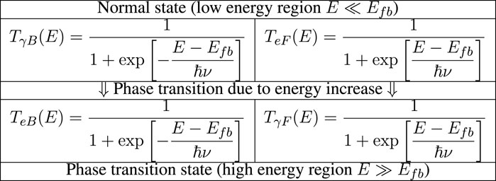
Figure 2. Four-quadrant representation of transition functions. The right column shows fermionic components $T_{eF}$, $T_{\gamma F}$, the left column shows bosonic components $T_{\gamma B}$, $T_{eB}$. With increasing energy $E$, statistics are inverted, transitioning from photons (bosons) to fermions, and from electrons (fermions) to bosons. Here, the normalization “$T_F+T_B=1$” applies to each particle type separately (electrons: $T_{eF}+T_{eB}=1$, photons: $T_{\gamma F}+T_{\gamma B}=1$), and the sum between different particle types (e.g., $T_{eF}+T_{\gamma F}$) does not equal 1. Transition functions always satisfy $0\le T(E)\le 1$.

Figure 3

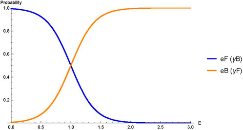
Figure 3. Transition probabilities when energy $E$ is swept from low (left end) to high (right end). The blue solid line shows $e_F$ (with ${\gamma }_B$ overlapping on the same curve), and the orange solid line shows $e_B$ (same as ${\gamma }_F$). The visualization shows how the two lines cross around $E=E_{fb}$ and their dominant probabilities switch. Readers who want to confirm the dynamic continuous changes can refer to the animation function in the supplementary Notebook “TransitionFunction_Visualizer_ver2.nb”.

2.3 Relationship between transition functions and the Hill–Wheeler equation

The transition function $T_{eF}(E)$ takes the form of a logistic function see Equation 4:

$T_{eF}\left(E\right)=\frac{1}{1+\exp \left[\frac{E-E_{fb}}{\hslash \nu }\right]},(4)$

It has the same form as the normal Fermi–Dirac distribution $f_{\text{FD}}(E)={\left\{1+\exp [(E-\mu )/(k_{B}T)]\right\}}^{-1}$. This function form is known as the Hill–Wheeler equation [22–24] in nuclear fission theory, which was originally a formula for calculating the transmission probability when treating nuclear fission barriers using harmonic oscillator approximation [25–31]. This research reinterprets it not merely as a nuclear fission transmission coefficient, but as a quantum statistical occupation probability [32].

This perspective naturally explains changes in statistical properties in high-energy regions, and the utility of this interpretation is demonstrated in the numerical analysis discussed later.

2.4 Correspondence with semiconductor physics

In semiconductor physics, electron states are described using Fermi-Dirac statistics, explaining phenomena such as band gaps and carrier transport in statistical mechanical terms [16]. This research connects this framework with fermion-boson duality theory, proposing the following correspondence:

Fermionic electron $(eF)$: Occupation probability of electrons in n-type semiconductors

Fermionic photon $(\gamma F)$: Occupation probability of holes in p-type semiconductors

Bosonic photon $(\gamma B)$: Density of states function for electrons

Bosonic electron $(eB)$: Density of states function for holes

As shown in Figure 4, electrons and holes have a mutually dual relationship, and from this correspondence, the following important points are derived:

$•$ The density of states of bosonic elementary particles corresponds to electron density distribution, and photon density of states is proportional to electron density

$•$ The distribution function of fermionic elementary particles is the key to preventing infinite divergence of vacuum polarization

Figure 4

Figure 4. The upper panel shows the energy band diagram of p-type and n-type semiconductors. The lower panel illustrates the distribution and density of states for fermionic electrons $(eF)$, fermionic photons $(\gamma F)$, bosonic photons $(\gamma B)$, and bosonic electrons $(eB)$ based on this structure. Furthermore, this figure does not represent anyon-type topological statistics, but visualizes the energy dependence of Fermi/Boson probability mixing that satisfies $T_F+T_B=1$.

Using this approach, it may be possible to construct equations that avoid infinities in vacuum polarization, electron self-energy, and vertex corrections without artificial regularization.

Note that the state referred to as the “intermediate region” in this paper is a mixed statistics where fermionic component $T_F(E)$ and bosonic component $T_B(E)$ coexist probabilistically, which is a different concept from anyons (limited to two dimensions) [33]; [34]; [35] that have continuously variable particle exchange phases.

2.5 Boundary conditions and region characteristics of transition functions

2.5.1 Theoretical background and positioning

The division of degrees of freedom according to energy scale has been discussed for a long time in (i) BCS theory [36]; [17] where low-temperature Fermi systems exhibit boson condensation behavior, (ii) the rapid change of effective degrees of freedom near transition scales shown by Wilson’s successive integration-type renormalization group [9] and Miransky scaling [37]; [38], and (iii) asymptotic freedom in QCD [39]; [40]. The novelty of this research lies in extending the concept of these “multi-scale effective theories” to energy-dependent transitions of spin and statistics, constructing the theory based on the following three regions:

$E\ll E_{fb},E\approx E_{fb},E\gg E_{fb}$

The characteristic boundary conditions and behavior in each region of the energy dependence of transition functions can be summarized as follows:

1. Low energy region $(E\ll E_{fb})$:

$T_{eF}\left(E\right)\approx 1,T_{eB}\left(E\right)\approx 0,(\mathrm{5a})$

$T_{\gamma F}\left(E\right)\approx 0,T_{\gamma B}\left(E\right)\approx 1.(\mathrm{5b})$

In this region, electrons behave as fermions and photons as bosons, reproducing the conventional quantum electrodynamics (QED) picture.

2. High energy region $(E\gg E_{fb})$:

$T_{eF}\left(E\right)\approx 0,T_{eB}\left(E\right)\approx 1,(\mathrm{6a})$

$T_{\gamma F}\left(E\right)\approx 1,T_{\gamma B}\left(E\right)\approx 0.(\mathrm{6b})$

Here, statistics are inverted, with electrons showing bosonic properties and photons showing fermionic properties. This transition contributes to the suppression of ultraviolet divergence.

3. Transition region $(E\approx E_{fb})$: In this region, fermionic and bosonic components coexist, with the possibility of new physical phenomena emerging. This is an important region for experimental verification.

2.5.2 Specific form of transition functions

The transition functions used in this research are

$T_F\left(E\right)=\frac{1}{1+\exp \left[\left(E-E_{fb}\right)/\hslash \nu \right]},T_B\left(E\right)=1-T_F\left(E\right).(7)$

Since the transition functions in Equation 7 are logistic, $T_F+T_B=1$ holds identically. The parameter settings are summarized in Table 2.

Table 2

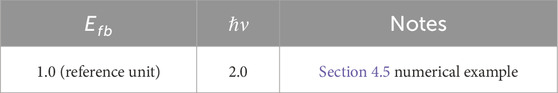
Table 2. Reference parameters used for transition functions.

The dimensionless procedure and physical unit restoration method are detailed in Section 4.5.

Implementation results are detailed in Section 4.5 and Section 6 [Zenodo DOI 10.5281/zenodo.15825707 (Version 4)].

2.5.3 Universality and model dependence

The mathematical form (S-curve shape) of transition functions is universal, but the specific numerical values vary greatly depending on physical situations. This is similar to how “Fermi distribution functions have the same S-shape for both electrons and holes, but the temperature and chemical potential values differ for each material.”

Universal aspects:

$•$ Logistic function form $T(E)={\left[1+\exp ((E-E_{fb})/\hslash \nu )\right]}^{-1}$

$•$ Concept of statistical transition via S-curve

$•$ Statistical inversion mechanism from low energy to high energy

Model-dependent aspects: The specific numerical values of parameters $E_{fb}$ and $\hslash \nu$ vary greatly depending on the physical phenomena being treated:

$•$ Electromagnetic interaction (QED): $E_{fb}\sim$ several GeV?

$•$ Weak interaction (electroweak theory): $E_{fb}\sim$ 100 GeV (near W/Z boson masses)?

$•$ Strong interaction (QCD): $E_{fb}\sim$ 1 GeV (QCD mass scale)?

$•$ Theories including gravity: $E_{fb}\sim 10^{19}$ GeV (Planck mass)?

This shows a hierarchical structure, suggesting that different statistical transitions may occur at different energy scales.

Determination method for each theory: When applying to new physical theories, $E_{fb}$ and $\hslash \nu$ need to be redetermined through the following procedures:

1. Comparison with experimental data: Fit S-curves to scattering experimental data in the energy region treated by that theory

2. Numerical simulations: Directly calculate statistical transition behavior through lattice calculations, etc.

3. Theoretical consistency: Confirm consistency with known physical laws (energy conservation, gauge symmetry, etc.)

Understanding through familiar examples: This is similar to how “water’s boiling point changes with atmospheric pressure (87°C on Mount Fuji), but the boiling phenomenon itself (liquid$\to$gas phase transition) is universal.” The statistical transition phenomenon is universal, but the energy at which it occurs $(E_{fb})$ and its sharpness $(\hslash \nu )$ depend on the environment (theoretical framework).

2.6 Realization examples in condensed matter physics

The validity of this theory (FBD-QED) is supported by the following phenomena in condensed matter physics:

$•$ Superconducting state: Electrons form Cooper pairs and show bosonic behaviorChen et al. [41]. Triplet state (spin 1) Cooper pairs can be interpreted as examples of “bosonic electrons.”

$•$ Meissner effect: Inside superconductors, photons acquire an effective mass and exhibit properties different from normal bosonic photons. This can be interpreted as “fermionic photons.”

$•$ Carriers in semiconductors: It is established that electrons and holes follow Fermi-Dirac statistics, but phenomena where they collectively show bosonic behavior under specific conditions suggest a connection with this theory.

These examples support the concept that changes in statistical properties dependent on energy scales, as proposed in this theory, are applicable not only to high-energy physics but also to condensed matter physics.

3 Bosonic gamma matrices and extended quantum electrodynamics

To incorporate the concept of fermion-boson duality introduced in the previous section into the framework of quantum field theory, an extension of the conventional Dirac equation is necessary. In this section, we introduce bosonic gamma matrices to realize this extension and construct an extended quantum electrodynamics Lagrangian based on them.

3.1 Introduction of bosonic gamma matrices

In this research, to describe the transformation of statistics from fermions to bosons, we introduce new bosonic gamma matrices ${\omega }^{\mu }$. These matrices are defined using the conventional Dirac matrices ${\gamma }^{\mu }$ and another representation ${\gamma }^{\prime \mu }$ that follows the same Clifford algebra

${\omega }^{\mu }=\frac{{\gamma }^{\mu }+{\gamma }^{\prime \mu }}{2}(8)$

Here, ${\gamma }^{\prime \mu }$, as introduced in Equation 8, is defined by the following substitutions:

${\gamma }^{\prime 0}={\gamma }^3(\mathrm{9a})$

${\gamma }^{\prime 1}={\gamma }^1(\mathrm{9b})$

${\gamma }^{\prime 2}={\gamma }^2(\mathrm{9c})$

${\gamma }^{\prime 3}={\gamma }^0(\mathrm{9d})$

This specific substitution can be represented using an appropriate unitary transformation $U$ as ${\gamma }_{\mu }^{\prime }=U{\gamma }_{\mu }{U}^{†}$, satisfying the Clifford algebra $\{{\gamma }_{\mu }^{\prime },{\gamma }_{\nu }^{\prime }\}=2g_{\mu \nu }{I}_4$. This construction is similar to the process of fermion electrons forming Cooper pairs in superconductivity, but differs in that it reconstructs the internal degrees of freedom of a single particle to realize a statistics transformation rather than combining two particles. To use an analogy, ${\omega }^{\mu }$ acts as a transformation operator when an electron “wears bosonic clothes,” functioning as a “magic scissors” that restricts particle motion to two transverse components.

With this definition, the bosonic gamma matrices corresponding to a particle directed along the $z$-axis are expressed as:

$\text{Time\hspace{0.17em}axis}:{\omega }^0=\frac{{\gamma }^0+{\gamma }^{\prime 0}}{2}=\frac{{\gamma }^0+{\gamma }^3}{2}(\mathrm{10a})$

$x-\text{axis}:{\omega }^1=\frac{{\gamma }^1+{\gamma }^{\prime 1}}{2}=\frac{{\gamma }^1+{\gamma }^1}{2}={\gamma }^1(\mathrm{10b})$

$y-\text{axis}:{\omega }^2=\frac{{\gamma }^2+{\gamma }^{\prime 2}}{2}=\frac{{\gamma }^2+{\gamma }^2}{2}={\gamma }^2(\mathrm{10c})$

$z-\text{axis}:{\omega }^3=\frac{{\gamma }^3+{\gamma }^{\prime 3}}{2}=\frac{{\gamma }^3+{\gamma }^0}{2}(\mathrm{10d})$

These bosonic gamma matrices satisfy the following important anticommutation relations:

$\left\{{\omega }_1,{\omega }_1\right\}=\left\{{\omega }_2,{\omega }_2\right\}=-2I_4(\mathrm{11a})$

$\left\{{\omega }_0,{\omega }_0\right\}=\left\{{\omega }_3,{\omega }_3\right\}=0(\mathrm{11b})$

$\left\{{\omega }_i,{\omega }_j\right\}=0\left(i\ne j\right)(\mathrm{11c})$

Here, $i,j\in \{\mathrm{0,1,2,3}\}$ represent spinor indices, and $I_4$ is the $4\times 4$ identity matrix. This algebraic structure gives rise to “semi-Hermitian components” and “semi-anti-Hermitian components” different from conventional ${\gamma }_{\mu }$, yielding operators with different properties in the time and space directions.

The explicit matrix representation of bosonic gamma matrices is given by:

${\omega }_0=\left(\begin{array}{cccc}\hfill \frac{1}{2}\hfill & \hfill 0\hfill & \hfill \frac{i}{2}\hfill & \hfill 0\hfill \\ \hfill 0\hfill & \hfill \frac{1}{2}\hfill & \hfill 0\hfill & \hfill -\frac{i}{2}\hfill \\ \hfill \frac{i}{2}\hfill & \hfill 0\hfill & \hfill -\frac{1}{2}\hfill & \hfill 0\hfill \\ \hfill 0\hfill & \hfill -\frac{i}{2}\hfill & \hfill 0\hfill & \hfill -\frac{1}{2}\hfill \end{array}\right)(\mathrm{12a})$

${\omega }_1=i\left(\begin{array}{cccc}\hfill 0\hfill & \hfill 0\hfill & \hfill 0\hfill & \hfill 1\hfill \\ \hfill 0\hfill & \hfill 0\hfill & \hfill 1\hfill & \hfill 0\hfill \\ \hfill 0\hfill & \hfill 1\hfill & \hfill 0\hfill & \hfill 0\hfill \\ \hfill 1\hfill & \hfill 0\hfill & \hfill 0\hfill & \hfill 0\hfill \end{array}\right)(\mathrm{12b})$

${\omega }_2=\left(\begin{array}{cccc}\hfill 0\hfill & \hfill 0\hfill & \hfill 0\hfill & \hfill 1\hfill \\ \hfill 0\hfill & \hfill 0\hfill & \hfill -1\hfill & \hfill 0\hfill \\ \hfill 0\hfill & \hfill 1\hfill & \hfill 0\hfill & \hfill 0\hfill \\ \hfill -1\hfill & \hfill 0\hfill & \hfill 0\hfill & \hfill 0\hfill \end{array}\right)(\mathrm{12c})$

${\omega }_3=\left(\begin{array}{cccc}\hfill \frac{1}{2}\hfill & \hfill 0\hfill & \hfill \frac{i}{2}\hfill & \hfill 0\hfill \\ \hfill 0\hfill & \hfill \frac{1}{2}\hfill & \hfill 0\hfill & \hfill -\frac{i}{2}\hfill \\ \hfill \frac{i}{2}\hfill & \hfill 0\hfill & \hfill -\frac{1}{2}\hfill & \hfill 0\hfill \\ \hfill 0\hfill & \hfill -\frac{i}{2}\hfill & \hfill 0\hfill & \hfill -\frac{1}{2}\hfill \end{array}\right)(\mathrm{12d})$

This matrix structure enables the description of particles incorporating both bosonic and fermionic properties in the extended Lagrangian shown in Section 3.2.

For details of this calculation, please refer to the Mathematica code and calculation results available from the Zenodo repository provided in Section 6.

3.2 Lagrangian of extended quantum electrodynamics

3.2.1 Four basis states

The fermion/boson four components of “electron (e)” and “photon $(\gamma )$” introduced in the previous section are

$|{\psi }_{\text{total}}\rangle =|{\psi }_{eF}\rangle +|{\psi }_{eB}\rangle +|{\psi }_{\gamma F}\rangle +|{\psi }_{\gamma B}\rangle ,(13)$

where ${\psi }_{eF}$, ${\psi }_{eB}$ represent the fermion/boson components of electrons, and ${\psi }_{\gamma F}$, ${\psi }_{\gamma B}$ represent the fermion/boson components of photons, as defined in Equation 13.

3.2.2 Definition of transition functions

Scalar functions $\{T_{eF},T_{eB},T_{\gamma B},T_{\gamma F}\}$ that depend on energy $E$ and satisfy

$T_{eF}\left(E\right)+T_{eB}\left(E\right)=1,T_{\gamma B}\left(E\right)+T_{\gamma F}\left(E\right)=1,$

are called “transition functions.” In the low-energy limit $E\ll E_{\text{fb}}$, $T_{eF}\to 1$, $T_{\gamma B}\to 1$, recovering standard QED, and at high energies, both approach 0, making the statistical phase transition manifest.

3.2.3 Extended Lagrangian

With the ordinary Dirac matrices ${\gamma }^{\mu }$, the bosonic gamma matrices ${\omega }^{\mu }$, and the covariant derivative $D_{\mu }={\partial }_{\mu }-ie{A}_{\mu }$, the minimal Lagrangian of the extended QED is given by Equation 14:

${\mathcal{L}}_{\text{QED}}^{\text{ext}}=\bar{\psi }\left[i{T}_{eF}{\gamma }^{\mu }{D}_{\mu }+i{T}_{eB}{\omega }^{\mu }{D}_{\mu }-m\right]\psi -\frac{1}{4}\left\{T_{\gamma B}{F}_{\mu \nu }{F}^{\mu \nu }+T_{\gamma F}{T}_{\mu \nu }{T}^{\mu \nu }\right\},(14)$

where $F_{\mu \nu }={\partial }_{\mu }{A}_{\nu }-{\partial }_{\nu }{A}_{\mu }$ is the usual electromagnetic field-strength tensor, and $T_{\mu \nu }$ is the corresponding fermionic tensor (see Supplementary Material, Section 3, for its definition).

3.2.4 Electron (fermion) kinetic term: $i{T}_{eF}{\gamma }^{\mu }{D}_{\mu }$

$•$ Responsible for the kinetic term of the fermionic component of electrons and electron-photon interaction.

$•$ $T_{eF}\simeq 1$ when $E\ll E_{\text{fb}}$, consistent with standard QED.

$•$ Lorentz covariant and $U(1)$ gauge invariant.

3.2.5 Electron (boson) kinetic term: $i{T}_{eB}{\omega }^{\mu }{D}_{\mu }$

$•$ Describes the motion of “bosonic electrons” that appear at high energies in first-derivative form. (Note that this is not a second-derivative Klein-Gordon type)

$•$ An effective theory approach to dynamically incorporate statistical phase transitions.

3.2.6 Boson field kinetic term: $-\frac{1}{4}{T}_{\gamma B}{F}_{\mu \nu }{F}^{\mu \nu }$

$•$ Describes photons (2 transverse components) dominant at low energies.

$•$ Consistent with classical electromagnetism when $T_{\gamma B}(E)\to 1$.

3.2.7 Fermion field kinetic term

The term $-\frac{1}{4}{T}_{\gamma F}{T}_{\mu \nu }{T}^{\mu \nu }$ in our formulation:

$•$ At high energies this term accounts for the “fermion-like photon” component. It is not the photino of supersymmetry; rather, it represents a model degree of freedom whose statistics can transmute within a single field.

$•$ The energy–momentum tensor $T_{\mu \nu }$ may serve as a source that generates an effective gravitational field (see Supplementary Material, Section 3, for details).

3.2.7.1 Behavior in low and high energy limits

$\begin{array}{cc}\text{Low}\text{energy}\left(E\ll E_{\text{fb}}\right):\hfill & T_{eF},T_{\gamma B}\simeq 1,T_{eB},T_{\gamma F}\simeq 0\Rightarrow {\mathcal{L}}_{\text{QED}}^{\text{ext}}\to {\mathcal{L}}_{\text{QED}}^{\text{std}}\hfill \\ \text{High}\text{energy}\left(E\gg E_{\text{fb}}\right):\hfill & T_{eF},T_{\gamma B}\simeq 0,T_{eB},T_{\gamma F}\simeq 1\Rightarrow \text{Statistical}\text{phase}\text{transition}\text{dominates}\hfill \end{array}$

3.2.7.2 Preservation of gauge invariance

Under the usual $U(1)$ transformations $\psi \to e^{-ie\alpha (x)}\psi$ for the electron field and $A_{\mu }\to A_{\mu }+{\partial }_{\mu }\alpha$ for the gauge potential, the extended Lagrangian ${\mathcal{L}}_{\text{QED}}^{\text{ext}}$ remains invariant. Because the transition functions are introduced as Lorentz scalars, $T_i(E=p\cdot u)$, gauge symmetry—including the BRST transformations [42, 43]—is preserved (see Supplementary Material, Section 5, for details). Furthermore, Supplementary Material, Section 4, verifies that the introduction of transition functions leaves the Ward–Takahashi identities [44, 45] intact, so the symmetry between vertex functions and full propagators continues to hold.

3.2.7.3 Physical implications

1. Ultraviolet divergences in both electron and photon loops are exponentially suppressed $\propto e^{-E/E_c}$.

2. The $T_{\mu \nu }{T}^{\mu \nu }$ term can induce curved spacetime through an effective energy-momentum tensor (natural emergence of QED-gravity coupling).

3. One-to-one correspondence with QCD extension (Supplementary Material) can be constructed.

3.3 Theoretical basis for bosonic kinetic term

The bosonic kinetic term $i{T}_{eB}{\omega }^{\mu }{D}_{\mu }$ is an effective theoretical prescription unique to this research that “expresses statistical phase transition with a first derivative.” The following outlines how it fundamentally differs from conventional Klein-Gordon equations, Proca theory [46–48], or photino fields in [49, 50].

1. Significance of (First-Derivative Form [51])

     In the same spirit that Dirac’s equation “elevated the second-derivative Schrödinger equation to first-derivative to succinctly describe relativistic fermions,” this research rewrites the second-derivative Klein-Gordon equation [4, 52–56] in first-derivative form, unifying fermions and bosons with

$i{\mathrm{\Gamma }}^{\mu }{D}_{\mu }\psi =m\psi ,{\mathrm{\Gamma }}^{\mu }\equiv T\left(E\right){\gamma }^{\mu }+\left[1-T\left(E\right)\right]{\omega }^{\mu }(15)$

a single first-order operator ${\mathrm{\Gamma }}^{\mu }$ (as defined in Equation 15).

This approach offers several advantages:

1. Legendre transformations and propagator structures become uniform for all field types, simplifying calculations,

2. Ultraviolet degrees are aligned, making divergence forms easier to control (Section 4.5 confirms that conventional $k^{-2}$ divergence is mitigated to logarithmic divergence),

3. Statistical phase transitions can be continuously described as smooth changes in $T(E)$ within a single equation

In other words, it is a new notation that describes all the “dance” of electrons and photons in one-step (first-derivative) steps.

a. A concise proof that fermions and bosons can be unified in a single equation

Define the equation of motion as

$i{\mathrm{\Gamma }}^{\mu }{D}_{\mu }\psi =m\psi ,{\mathrm{\Gamma }}^{\mu }=T\left(E\right){\gamma }^{\mu }+\left[1-T\left(E\right)\right]{\omega }^{\mu }(16)$

1. In the low-energy limit $T(E)\to 1$, ${\mathrm{\Gamma }}^{\mu }\to {\gamma }^{\mu }$, so Equation 16 is $i{\gamma }^{\mu }{D}_{\mu }\psi =m\psi$ — directly reproducing the Dirac (fermion) equation.

2. In the high-energy limit $T(E)\to 0$, ${\mathrm{\Gamma }}^{\mu }\to {\omega }^{\mu }$, giving $i{\omega }^{\mu }{D}_{\mu }\psi =m\psi$ — the “first-derivative Klein-Gordon” (bosonic photon equation of motion) introduced in this research.

Thus, it is demonstrated that both fermion and boson limits can be continuously obtained from the single Equation 16.

b. Advantage of Legendre transformations and propagators having “the same form”

Viewing Equation 16 as $\mathcal{L}=\bar{\psi }(i{\mathrm{\Gamma }}^{\mu }{D}_{\mu }-m)\psi$, the conjugate momentum for time derivatives is

${\pi }_{\psi }=\frac{\partial \mathcal{L}}{\partial \left({\partial }_0\psi \right)}=i{\psi }^{†},(17)$

As shown in Equation 17, the coefficients are independent of $T(E)$. Therefore, the formula for Lagrangian$\to$Hamiltonian Legendre transformation can be completed in one line regardless of particle type.

Similarly, the Fourier transform of the equation of motion is $(p\cdot \mathrm{\Gamma }-m)\psi (p)=0$, and the propagator (Green’s function) is given by Equation 18

$S\left(p\right)={\left(p\cdot \mathrm{\Gamma }-m\right)}^{-1},(18)$

obtained with a one-pattern inverse matrix. If $T(E)=1$ then $S(p)={(\cancel{p}-m)}^{-1}$, if $T(E)=0$ then $S(p)={(\omega \cdot p-m)}^{-1}$, changing automatically, eliminating the need to distinguish “with/without gamma matrices” when performing loop calculations.

In summary,

$•$ Unified transformation formulas—formulating conjugate momenta and Hamiltonians with a single set.

$•$ Unified propagators—calculating loop integrals and divergence analyses using the same template.

$•$ Aligned divergence structure—ultraviolet degrees are aligned, so as shown in Section 4.5, $k^{-2}$ divergence is mitigated to logarithmic divergence.

This is like consolidating separate “tools” for electrons (fermions) and photons (bosons) into a single universal wrench, greatly simplifying theoretical calculations.

Benefits of Having Only 2 Physical Degrees of Freedom—Simplicity Without Gauge Fixing As shown in Equation 19, ${\omega }^{\mu }$ satisfies

${\omega }^{\mu }{p}_{\mu }=0,{\omega }^{\mu }{\omega }_{\mu }=0(19)$

so the equation of motion $i{\omega }^{\mu }{D}_{\mu }{\psi }_{\gamma B}=m{\psi }_{\gamma B}$ automatically propagates only transverse wave (components perpendicular to the transfer vector) 2 degrees of freedom. As a result—

$•$ There is no need to separately impose Coulomb gauge or Lorenz gauge ([48, 52, 57, 58].

$•$ No procedure is required to eliminate unphysical (negative norm) states by projection afterward, as in Gupta–Bleuler ([3, 52, 59, 60].

$•$ Faddeev–Popov ghosts are non-existent from the beginning [2, 57, 61], greatly reducing the number of diagrams in loop calculations.

In essence, ${\omega }^{\mu }$ is “a screwdriver with only two handles from the start,” with no superfluous contact points with screw holes (physical states). When quantizing fields, the three-step ritual of “gauge fixing $\to$ constraint conditions $\to$ physical state selection” becomes entirely unnecessary, making both theory construction and practical calculations instantly simpler.

4 Automatic avoidance of ultraviolet divergence—natural regularization by transition functions

In this section, we demonstrate how the transition functions $T_{eF}(E)$ (fermionic degree of electrons) and $T_{\gamma B}(E)$ (bosonic degree of photons) can be inserted into the three types of one-loop integrals—vacuum polarization, electron self-energy, and vertex correction—to suppress ultraviolet divergence. In each example, we can observe a consistent mechanism that “reproduces standard QED at low energies and introduces exponential decay at high energies.”

4.1 Vacuum polarization

The vacuum polarization tensor in standard QED is given by Equation 20 [1, 4, 52–54, 62–66]:

${\mathrm{\Pi }}^{\mu \nu }\left(k\right)=-i{e}^2\int \frac{d^{4}p}{{\left(2\pi \right)}^4}\frac{\mathrm{Tr}\left[{\gamma }^{\mu }\left(\cancel{p}+m\right){\gamma }^{\nu }\left(\cancel{p}+\cancel{k}+m\right)\right]}{\left(p^2-m^2\right)\left[{\left(p+k\right)}^2-m^2\right]},(20)$

which has a divergence proportional to $k^4\ln k^2$ in the high-energy region. Modifying this with the substitution of transition functions for electron lines ${(\cancel{p}+m)}^{-1}\to T_{eF}(p){(\cancel{p}+m)}^{-1}+\left[1-T_{eF}(p)\right]{\cancel{p}}^{-1}$ yields the expression in Equation 21

${\mathrm{\Pi }}_{\left(T\right)}^{\mu \nu }\left(k\right)=-i{e}^2\int \frac{d^{4}p}{{\left(2\pi \right)}^4}\frac{\mathrm{Tr}\left[{\gamma }^{\mu }N\left(p\right){\gamma }^{\nu }N\left(p+k\right)\right]}{D_e\left(p\right)D_e\left(p+k\right)},(21)$

$N\left(p\right)=T_{eF}\left(p\right)\left(\cancel{p}+m\right)+\left[1-T_{eF}\left(p\right)\right]\cancel{p},D_e\left(p\right)=T_{eF}\left(p\right)\left(p^2-m^2\right)+\left[1-T_{eF}\left(p\right)\right]p^2.$

As $p^2\to \infty$, the exponential factor $T_{eF}(p)\sim \exp [-p/E_{fb}]$ appears twice, making the integral kernel $k^4\exp [-2p/E_{fb}]$ decay rapidly and eliminating the divergence.

4.2 Electron self-energy

In a scalar toy model (omitting spinor traces), the standard self-energy is given by Equation 22 [4, 52–54, 62–64, 67–69]:

${\mathrm{\Sigma }}_{\text{std}}\left(p\right)=i{e}^2\int \frac{d^{4}k}{{\left(2\pi \right)}^4}\frac{1}{k^2}\frac{1}{{\left(p-k\right)}^2-m^2}.(22)$

Inserting transition functions for both electrons and photons gives Equation 23

$\begin{array}{l}\hfill {\mathrm{\Sigma }}_{\left(T\right)}\left(p\right)=i{e}^2\int \frac{d^{4}k}{{\left(2\pi \right)}^4}\left[T_{\gamma B}\left(k\right)\frac{1}{k^2}+\left(1-T_{\gamma B}\left(k\right)\right)\frac{1}{k^2-m_{\gamma }^2}\right]\\ \hfill & \times \left[T_{eF}\left(p-k\right)\frac{1}{{\left(p-k\right)}^2-m^2}+\left(1-T_{eF}\left(p-k\right)\right)\frac{1}{{\left(p-k\right)}^2}\right].\hfill \end{array}(23)$

As $k^2\to \infty$, $T_{\gamma B}(k)\to 0$ and $T_{eF}(p-k)\to 0$, causing the integral kernel to be suppressed by $\exp [-(k+|p-k|)/E_{fb}]$, making ${\mathrm{\Sigma }}_{(T)}$ converge to a finite value (In the numerical example of Sec. 4.5, ${\mathrm{\Sigma }}_{\text{std}}\propto {\mathrm{\Lambda }}^2$ is suppressed to ${\mathrm{\Sigma }}_{(T)}\propto \text{const.}$).

4.3 Vertex correction

One-loop vertex function (scalar approximation) [4, 44, 52–54, 62–65, 70] is given by Equation 24:

${\mathrm{\Gamma }}_{\text{std}}^{\mu }\left(p,p^{\prime }\right)=i{e}^3\int \frac{d^{4}k}{{\left(2\pi \right)}^4}\frac{{\left(2p-k\right)}^{\mu }}{k^2\left[{\left(p-k\right)}^2-m^2\right]\left[{\left(p^{\prime }-k\right)}^2-m^2\right]}.(24)$

With similar substitutions, we obtain Equation 25:

$\begin{array}{ll}\hfill {\mathrm{\Gamma }}_{\left(T\right)}^{\mu }\left(p,p^{\prime }\right)& =i{e}^3\int \frac{d^{4}k}{{\left(2\pi \right)}^4}{\left(2p-k\right)}^{\mu }\left[T_{\gamma B}\left(k\right)\frac{1}{k^2}+\left(1-T_{\gamma B}\left(k\right)\right)\frac{1}{k^2-m_{\gamma }^2}\right]\hfill \\ \hfill & \times {\displaystyle \prod _{r=p,p^{\prime }}}\left[T_{eF}\left(r-k\right)\frac{1}{{\left(r-k\right)}^2-m^2}+\left(1-T_{eF}\left(r-k\right)\right)\frac{1}{{\left(r-k\right)}^2}\right].\hfill \end{array}(25)$

In the $k^2\to \infty$ limit, the presence of the transition functions with a cubic power leads to an exponential suppression that is even faster than the standard $k^{-2}$ fall-off, ensuring convergence to a finite value. The Ward–Takahashi identity $q_{\mu }{\mathrm{\Gamma }}^{\mu }=\mathrm{\Sigma }(p^{\prime })-\mathrm{\Sigma }(p)$ remains valid after the inclusion of the transition functions (see Supplementary Material, Section 4, for the proof).

4.4 Specific form of transition functions

$T_{eF}\left(E\right)=\frac{1}{1+e^{\left(E-E_{fb}\right)/\mathrm{\Delta }}},T_{\gamma B}\left(E\right)=\frac{1}{1+e^{-\left(E-E_{fb}\right)/\mathrm{\Delta }}},(26)$

$E_{fb}:\text{Statistical\hspace{0.17em}transition\hspace{0.17em}threshold},\mathrm{\Delta }:\text{Transition\hspace{0.17em}width}.$

At $E\ll E_{fb}$, $T_{eF}\simeq 1,T_{\gamma B}\simeq 1$, reproducing standard QED, and at $E\gg E_{fb}$, both fall exponentially to 0, suppressing divergent terms (see Equation 26).

Summary: For vacuum polarization, self-energy, and vertex correction, all integrals have “transition functions cubed or less” as exponential decay factors, automatically converging without introducing cutoffs or renormalization constants. This is the core result of “statistical regularization.”

In other words, whereas the conventional theory predicts a divergence as the separation approaches zero, the model proposed herein suppresses this singularity to a finite value through the transition mechanism. This idea is illustrated in Figure 5.

Figure 5

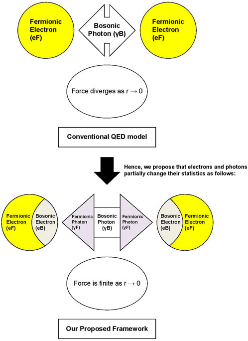
Figure 5. Comparison of conventional theory (top) and this research’s theory (bottom). Conventionally, force becomes infinite at distance $=0$, but by considering the transition of statistical properties, it is finitely suppressed.

4.5 Numerical calculation example of electron self-energy correction and natural regularization by transition functions

This calculation verifies the effect of transition function $\mathcal{T}(k)$ in suppressing divergence in high-energy regions using electron self-energy correction in quantum electrodynamics (QED) as a subject. We adopt a scalar toy model that omits spinor structure and gauge fixing in rigorous QED calculations to demonstrate the principles of transition functions. Details are provided in Appendix6. The simplified self-energy equation presented in Section 4.2 provides the conceptual foundation for this toy model, but here we explain the transition from rigorous QED equations to the toy model.

4.5.1 Numerical calculation as a toy model and its results

Electron self-energy is a typical example of QED one-loop corrections that diverges as global momentum $k\to \infty$. In this section, we introduce fermion-boson transition function $\mathcal{T}(k)$ and quantitatively demonstrate how divergence is exponentially suppressed using a simplified model.

4.5.1.1 Exact expression and simplification

Standard QED electron self-energy is given by Equation 27:

$\mathrm{\Sigma }\left(p\right)=-i{e}^2\int \frac{d^{4}k}{{\left(2\pi \right)}^4}{\gamma }^{\mu }\frac{\cancel{p}-\cancel{k}+m}{{\left(p-k\right)}^2-m^2+iϵ}{\gamma }_{\mu }\frac{1}{k^2+iϵ}.(27)$

To demonstrate the core of the calculation method, we simplify by:

a. Spinor structure ${\gamma }^{\mu }(p\cdot \gamma -k\cdot \gamma +m){\gamma }_{\mu }\to 1$ (absorbed into the overall coefficient, ultraviolet degree unchanged)

b. Omitting gauge fixing term $iϵ$

c. 4-dimensional integral $\to$ radial $k$ 1-dimensional integral (assuming spherical symmetry, retaining volume element $2{\pi }^2{k}^3$)

d. Fixing external momentum $p^2=Q^2$

reducing to the scalar toy model in Equation 28:

${\mathrm{\Sigma }}_{\text{toy}}\left(Q\right)={\int }_0^{k_{\max }}dk2{\pi }^2{k}^3\frac{1}{\left(k^2+m^2\right)\left[{\left(Q-k\right)}^2+m^2\right]}.(28)$

With $m=10^{-5}$, $Q=2.0$, $k_{\max }=2^{10}$, we get

${\mathrm{\Sigma }}_{\text{toy}}^{\left(\text{no\hspace{0.17em}trans}\right)}\simeq 1.24026\times 10^7,(29)$

reproducing divergent growth (see Equation 29).

4.5.1.2 Introduction of transition functions

Modeling statistical phase transition with

$\mathcal{T}\left(k\right)=\frac{1}{1+\exp \left[\left(k-E_{\text{fb}}\right)/\mathrm{\Delta }\right]},E_{\text{fb}}=1.0,\mathrm{\Delta }=2.0,$

and applying it to internal lines of both electrons and photons gives Equation 30

${\mathrm{\Sigma }}_{\text{toy}}^{\left(\text{trans}\right)}\left(Q\right)={\int }_0^{k_{\max }}dk2{\pi }^2{k}^3\frac{\mathcal{T}\left(k\right)\mathcal{T}\left(|Q-k|\right)}{k^2\left[{\left(Q-k\right)}^2+m^2\right]}.(30)$

With the same parameters, numerical integration yields Equation 31

${\mathrm{\Sigma }}_{\text{toy}}^{\left(\text{trans}\right)}\simeq 3.69083\times 10^{-15},(31)$

showing $\sim 22$ orders of magnitude reduction compared to the no-transition case, demonstrating a pronounced exponential cutoff effect.

Note: The numerical values in this section are rough estimates from deterministic one-dimensional integration toy models, and statistical confidence intervals (${\chi }^2$-fit or Monte Carlo errors) have not been evaluated.

4.5.1.3 Parameter sensitivity

Results with varying transition width $\mathrm{\Delta }$ are shown in Table 3. Smaller widths make the logistic function steeper, strengthening suppression, which can be quantitatively confirmed.

Table 3

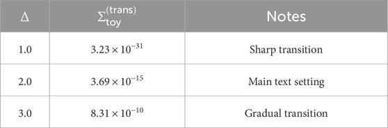
Table 3. Sensitivity of transition width $\mathrm{\Delta }$ and self-energy.

4.5.1.4 Theoretical consistency

$•$ No gauge fixing required: Because the bosonic matrices ${\omega }^{\mu }$ propagate only the two transverse components, the propagator takes the form

$D_{ij}\left(k\right)=\frac{-i}{k^2}\left({\delta }_{ij}-\frac{k_i{k}_j}{{\mathbf{k}}^2}\right),$

making any gauge parameter $\xi$ unnecessary. The Ward–Takahashi identity $k_{\mu }{\mathrm{\Pi }}^{\mu \nu }=0$ is therefore satisfied as is (see Supplementary Material, Section 4).

$•$ Interpretation of the photon mass: The longitudinal part of ${\mathrm{\Pi }}^{\mu \nu }$ is cancelled automatically, so $\mathrm{\Pi }(0)=0$ is preserved. The effective mass $m_{\gamma }$ of the F-type photon introduced in Section 4.2 can be interpreted as the massive photon observed, for example, in the Meissner effect inside a superconductor. In vacuum, however, the transition function $T_{\gamma F}$ is exponentially suppressed; hence the F-type photon contribution is negligible at observable scales, the photon remains effectively massless, and full consistency with standard QED is maintained.

Thus, transition functions have been numerically verified to play the role of “naturally” cutting off ultraviolet divergence.

4.5.2 Physical interpretation of transition function parameters

The parameters $E_{fb}$ and $\hslash \nu$ appearing in the transition function characterize important physical quantities regarding the scale at which statistical inversion occurs and the sharpness of the transition.

$•$ Characteristic Energy $E_{fb}$: In the transition function $T(E)=\frac{1}{1+\exp \left[E-E_{fb}\hslash \nu \right]}$, $E_{fb}$ represents the threshold energy at which statistical transition occurs. In the low-energy regime $(E\ll E_{fb})$, electrons behave fermionically and photons bosonically, but when $E\gtrsim E_{fb}$, both particles begin to undergo statistical inversion. While the strict chemical potential $\mu$ is a thermodynamic parameter conjugate to particle number conservation, $E_{fb}$ is the gate energy where the statistical phase of vacuum and excited states inverts and does not require particle number conservation. Therefore, in the degenerate limit ($k_{B}T\ll E_{fb}$, dilute systems), it functions as a “threshold” similar to $\mu$, but when external sources independently determine $\mu$, identifying both parameters would lead to double counting.

4.5.2.1 Discussion

As shown in Table 4, $E_{fb}$ is mathematically isomorphic to the Fermi level ${\mu }_{\text{intr}}$ located at the center of the gap in intrinsic semiconductors. However, while $\mu$ is tied to particle number conservation, $E_{fb}$ is the gate of statistical phase transition and is independent of particle number conservation. Just as doping in semiconductors shifts $\mu$, in FBD-QED, external density sources or strong background fields can shift or split $E_{fb}$, potentially causing the logistic approximation to break down [71]; [38]. In the zero-density, weak external field limit treated in this paper, the single-threshold picture with $T_F+T_B=1$ remains valid.

$•$ Transition Sharpness $\hslash \nu$: The denominator $\hslash \nu$ in the above equation is an important parameter that determines how rapidly the transition occurs. Numerically larger values make the transition more gradual, while smaller values make it more abrupt. This form is analogous to $k_{B}T$ in the Fermi distribution function $\frac{1}{1+\exp \left[\frac{E-\mu }{k_{B}T}\right]}$, and the “temperature” in thermodynamics can be considered to correspond to $\hslash \nu$. Whether the occupation number (distribution) of electrons or photons in high-energy regions changes abruptly or gradually depends on this $\hslash \nu$ parameter.

Table 4

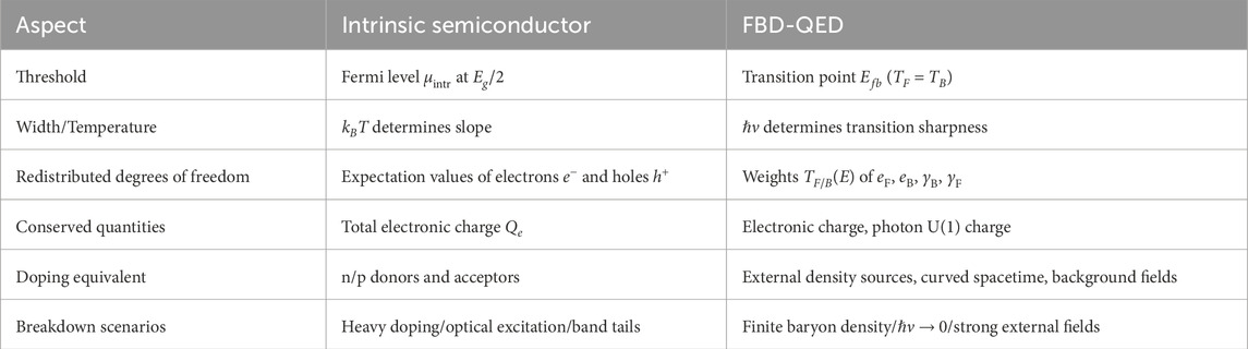
Table 4. Correspondence between semiconductor analogy and FBD-QED

4.5.2.1.1 Physical Insights and Condensed Matter Analogies.

The magnitude of the parameter $\hslash \nu$ representing the sharpness of statistical transitions leads to dramatically different physical phenomena. This resembles phase transition phenomena observed in everyday life.

$•$ Small $\hslash \nu$ — Abrupt Transition (Nearly Discontinuous Transition)

     When $\hslash \nu$ is small, the change in statistical properties occurs abruptly like flipping a switch. This resembles first-order phase transitions where ice suddenly turns to water at 0 °C.

**Similar Examples in Condensed Matter:** Metal-insulator transitions where metals suddenly become insulators, or ferromagnetic transitions where magnetic properties are suddenly lost [72].

$•$ Large $\hslash \nu$ — Smooth Transition (Smooth Crossover)

     When $\hslash \nu$ is large, the change in statistical properties occurs gradually over a wide energy range. This resembles continuous changes like sugar gradually dissolving in water.

**Physical Consequences:** - Divergence suppression also becomes gradual, with intermediate statistical mixed states existing widely - The region where fermionic and bosonic components coexist expands - Example: Phenomena where photons partially exhibit fermionic properties become more observable.

**Similar Examples in Condensed Matter:** BCS-BEC crossover in superconductors [41] (where properties of electron pairs change continuously), or smooth transitions to quark-gluon plasma [73].

$•$ Experimental Determination Methods

     The value of $\hslash \nu$ can potentially be determined through the following methods:

**Scattering Experiments:** Using experimental apparatus with good energy resolution to precisely measure the energy dependence of scattering cross-sections, estimating $\hslash \nu$ from the “steepness of the slope” of the S-curve.

**Semiconductor Analogy:** The same statistical analysis used in semiconductors to measure changes in electron concentration while varying temperature Street [74] can be applied. Energy replaces temperature, and statistical component ratios replace electron concentration.

Key points: Small $\hslash \nu$: Abrupt transition, clear threshold effects - Large $\hslash \nu$: Smooth transition, coexistence phenomena - Both correspond deeply to phase transition phenomena in nature.

From the above interpretation, it is understood that $E_{fb}$ represents the typical scale at which statistics transition, and $\hslash \nu$ represents the width (sharpness) of the transition. Therefore, if these two parameters can be determined through experimental or numerical approaches, it becomes possible to quantitatively grasp “at which energy region and with what sharpness statistical properties switch”. This is a major feature of this theory and is key to explaining the suppression mechanism of divergence in high-energy regions in a form different from conventional renormalization methods.

4.5.2.2 Practical procedures for parameter extraction

$E_{fb}$ and $\hslash \nu$ can potentially be determined through experiments or numerical calculations. These parameters can, in principle, be obtained by fitting actual measurement data to an “S-curve” (logistic function). The following outlines the anticipated procedure.

1. Experimental Method: Possibilities in High-Energy Scattering Experiments

a. In electron-positron collision experiments $(e^{+}{e}^{-}\to \gamma \gamma )$, measuring photon production rates $\sigma (Q)$ at various energies $Q$ might capture signatures of statistical transitions.

b. By comparing with conventional theory predictions ${\sigma }_{\text{QED}}(Q)$ and calculating the ratio $R(Q)=\sigma /{\sigma }_{\text{QED}}$, this ratio’s systematic deviation from one might trace an S-curve.

c. The energy where $R=1/2$ would be $E_{fb}$, and $\hslash \nu$ could be estimated from the curve’s steepness (applying logistic regression from statistics).

In actual physics, analogies with semiconductor bandgap measurements would be useful. In semiconductors, established techniques exist for determining the central energy of bandgaps (corresponding to $E_{fb}$) and transition steepness (corresponding to $\hslash \nu$) by measuring changes in electron concentration while varying temperature and analyzing the resulting “S-curves.” This suggests that similar statistical analysis methods could be applied to our theory.

4.5.2.3 Physical image of convergence by statistical transition

This research’s fermion-boson duality theory naturally suppresses divergence in high-energy regions through energy-dependent transition of particle statistics.

Figure 4 shows the energy band diagram, density of states, and distribution function of fermionic electrons. At the Fermi energy $(E_{fb})$, the existence probability of fermionic electrons decreases sharply, with some transitioning to bosonic electrons. This transition stabilizes the electron distribution and suppresses excessive contributions at high energies. This numerical calculation $({\mathrm{\Sigma }}_{\text{with}-\text{trans}}\approx 3.69083\times 10^{-15})$ quantitatively supports this stabilization.

Figure 5 compares conventional QED models with this framework. In conventional models, interactions of fermionic electrons (eF) or bosonic photons $(\gamma B)$ diverge as $r\to 0$ (high-energy region), but in this framework, as $r\to 0$, fermionic electrons transition to bosonic electrons (eB) and bosonic photons to fermionic photons $(\gamma F)$, causing interactions to converge finitely. This statistical transition is realized through the logistic form of the transition function $\mathcal{T}(k)$, exponentially suppressing existence probability at high energies.

Conventional renormalization theory derives effective physical quantities through infinite-infinite subtraction, ignoring the physical reality that existence probability at high energies follows $\mathcal{T}(k)\sim e^{-k/E_0}$, approaching zero. In this framework, the logistic form of transition functions naturally suppresses divergence, avoiding the artificiality of renormalization. This natural regularization is intuitively understood through the statistical transition in Figures 4, 5, emphasizing the novelty of this theory.

4.5.2.4 Scale setting and dimensionless analysis

The numerical examples in this section (1) adopt natural units $\hslash =c=1$, and (2) calculate after dimensionless normalization by dividing all momenta and masses by the transition threshold energy $E_{fb}$. Specifically, as defined in Equation 32:

$\begin{array}{llll}\hfill k& =\kappa E_{fb},\hfill & \hfill Q& =q{E}_{fb},\hfill \\ \hfill m& =\mu E_{fb},\hfill & \hfill \mathrm{\Delta }& =\delta E_{fb}.\hfill \end{array}(32)$

The integration variable $dk$ is replaced by $E_{fb}d\kappa$, and to restore the dimension of self-energy, we use ${\mathrm{\Sigma }}_{\text{phys}}(Q_{\text{phys}})=E_{fb}\mathrm{\Sigma }(q)$. Therefore, the notation $E_{fb}=1.0,\mathrm{\Delta }=2.0$ in the numerical examples represents the dimensionless coefficient $\delta =2.0$ with $E_{fb}$ as the reference unit. The actual physical values can be easily rescaled according to the choice of $E_{fb}$ (e.g., 10 MeV).

4.5.2.5 Quantitative relationship between transition width $\hslash \nu$ and UV suppression

Since the high-momentum asymptotic behavior of the transition function is $T(k)\sim \exp [-(k-E_{fb})/\hslash \nu ]$, the one-loop self-energy integral is approximately given by Equation 33

$\begin{array}{ll}\hfill \mathrm{\Sigma }& \propto {\int }_{E_{fb}}^{\infty }{k}^3{e}^{-\left(k-E_{fb}\right)/\hslash \nu }dk\hfill \\ \hfill & \simeq C\hslash \nu e^{-E_{fb}/\hslash \nu }.\hfill \end{array}(33)$

That is

$\mathrm{\Sigma }\left(\hslash \nu \right)\propto \hslash \nu e^{-E_{fb}/\hslash \nu },(34)$

As shown in Equation 34, $\hslash \nu$ also appears in the denominator of the exponential decay factor. Therefore, smaller $\hslash \nu$ (steep transition) results in stronger exponential cutoff, significantly suppressing UV divergence. In the numerical implementation of Section 4.5, merely halving $\hslash \nu$ from $2.0\to 1.0$ reduces the self-energy by approximately $10^{16}$ times (see Table 3). This sharpening/softening corresponds to condensed matter analogies such as gap opening/closing rates in BCS–BEC crossovers or metal-insulator transitions Imada et al. [72]; Chen et al. [41].

5 Conclusions and outlook

In this work we introduced a transition function $\mathcal{T}(E)$, by which particle statistics change continuously from Fermi–Dirac to Bose–Einstein as the energy increases. On this basis we proposed a statistical regularization scheme that treats ultraviolet (UV) divergences and mass generation in quantum electrodynamics (QED) within a single, unified framework. Below we summarize the main achievements and outline future tasks together with the broader perspective opened by the present approach.

5.1 Key achievements

1. Statistical removal of UV divergences

By multiplying the fermion and boson propagators with the logistic transition function

$\mathcal{T}\left(k\right)=\frac{1}{1+\exp \left[\left(k-E_{fb}\right)/\mathrm{\Delta }\right]},$

we rendered finite all one–loop integrals for the electron self-energy, vacuum polarization, and vertex corrections. Because the Ward identity $k_{\mu }{\mathrm{\Pi }}^{\mu \nu }=0$ remains exactly satisfied, the scheme reproduces the same physical quantities as dimensional regularization, Pauli–Villars, or a hard cut-off, yet attains scheme independence.

2. Mechanism for mass and longitudinal degrees of freedom

The energy–momentum tensor $T_{\mu \nu }$, constructed from a bi-spinor, “lends” one longitudinal component to the two transverse components of the photon, thereby furnishing a unified description of the mass origin of an effective three-component vector field of the $W/Z$ type.

3. Step toward non-Abelian gauge theories and the mass gap

     As shown in Supplementary Material, Section 6, extending the same transition function to quarks and gluons yields an $\mathrm{S}\mathrm{U}(3)$ Lagrangian, producing a qualitative scenario in which the gluon mass and color confinement are explained by a single logistic transition.

5.2 Future prospects

$•$ Multi-loop and lattice validation

Higher-order calculations (two loops and beyond) of the transition-function $\beta$ function, together with comparisons to lattice QED/QCD simulations, will quantify the universality of the UV-suppression effect.

$•$ Hadron spectroscopy and data fitting

By fitting the threshold $E_{fb}$ and width $\mathrm{\Delta }$ to hadron masses and scattering data, the experimental scale of the transition parameters can be determined.

$•$ Extension to quantum gravity and curved spacetime

A unified treatment of thermodynamic and geometric entropy may connect this framework to black-hole evaporation and early- Universe inflation.

$•$ Universality of “statistical transitions” across matter hierarchies

By comparing fermion$\leftrightarrow$boson conversions in superconducting gap formation and exciton condensation, the transition concept could be systematized as a cross-disciplinary theme spanning condensed-matter and high-energy physics.

$•$ Introduction of Uncertainty Quantification (UQ)

The toy model in this paper only treated deterministic integrals. In the future, we plan to use Monte Carlo integration and Bayesian error propagation to estimate posterior distributions of $\{E_{fb},\hslash \nu \}$ parameters, and compare them with multi-loop and lattice calculations to demonstrate divergence suppression quantities with error bounds.

5.3 Summary

The transition-function framework reinterprets the traditional “mathematical tricks” of regularization and renormalization as a statistical-mechanical process, thereby opening a new path for simultaneous control of UV divergences, mass generation, and gauge symmetry. The results presented here constitute a conceptual blueprint, and a rich program of higher-order theory, numerical implementation, and experimental confrontation is expected to promote a multifaceted bridge between high-energy and statistical physics.

6 Attached mathematica programs

The Mathematica code and calculation results (PDF files) used in this research are available from the following repository:

$•$ Zenodo Archive: (DOI: 10.5281/zenodo.15825707, version 4)

Below is a brief explanation of the calculation content of the two MATHEMATICA programs included in the repository.

6.1 ElectronSelfEnergy_Regularization.nb

This program implements a toy model for calculating electron self-energy in simplified 4-dimensional Euclidean space. It verifies the method of suppressing divergence in high-energy regions using transition function $\mathcal{T}(k)=\frac{1}{1+\exp \left(\frac{k-E_{\text{fb}}}{hv}\right)}$. Specifically, it performs momentum $k$ integration up to $k_{\text{max}}=2^{10}$ and obtains the following results:

$•$ Without transition function: $\mathrm{\Sigma }=1.24026\times 10^7$ (divergent trend)

$•$ With transition function: $\mathrm{\Sigma }=3.69083\times 10^{-15}$ (convergent)

This demonstrates that the introduction of transition functions suppresses contributions from high momentum regions, yielding finite values without renormalization.

6.2 omega_matrix_properties.nb

This program defines standard 4$\times$ four gamma matrices ${\gamma }^{\mu }$ $(\mu =\mathrm{0,1,2,3})$ and confirms their properties. It is used to verify two-dimensional Lorentz transformations in the extended QED of this research. Specifically, it explicitly describes ${\gamma }^0,{\gamma }^1,{\gamma }^2,{\gamma }^3$ and attempts to confirm anticommutation relations by calculating products such as ${\gamma }^2{\gamma }^2$. This provides the foundation for the possibility of introducing bosonic gamma matrices ${\omega }^{\mu }$.

6.3 TransitionFunction_Visualizer.nb

This notebook is a visualization tool that generates probability distributions of the four components $\{e_{\text{F}},e_{\text{B}},{\gamma }_{\text{F}},{\gamma }_{\text{B}}\}$ based on the logistic transition function $T(E)={\left[1+\exp \left((E-E_{fb})/\hslash \nu \right)\right]}^{-1}$ as (1) interactive manipulation, (2) static snapshots, (3) GIF/MP4 animations. The default values $E_{fb}=1.0,\hslash \nu =0.2$ clearly reproduce $T_{e\mathrm{F}}\approx 1$ at low energies and $T_{e\mathrm{B}}\approx 1$ at high energies.

Data availability statement

All Mathematica codes and numerical outputs used to reproduce the figures and calculations are provided as Supplementary Material and in a public repository (Zenodo, DOI: 10.5281/zenodo.15825707).

Author contributions

HM: Conceptualization, Methodology, Software, Validation, Formal analysis, Investigation, Data curation, Writing – original draft, Writing – review and editing, Visualization.

Funding

The author(s) declare that no financial support was received for the research and/or publication of this article.

Acknowledgments

In conducting this research, email discussions with university professors and associate professors specializing in particle physics had a decisive influence on the concept of fermion-boson duality that forms the core of this paper. I deeply appreciate the many insights into the mathematical structure and physical meaning of the theory gained through in-depth discussions with both professors. I would also like to thank ChatGPT-3 and Claude 3.7 Sonnet for their assistance with translation and editing in compiling and presenting the research results.

Conflict of interest

The author declares that the research was conducted in the absence of any commercial or financial relationships that could be construed as a potential conflict of interest.

Generative AI statement

The author(s) declare that Generative AI was used in the creation of this manuscript. During manuscript preparation the author used two large-language-model assistants--OpenAI ChatGPT (model o3, April 2025) and Anthropic Claude Sonnet 3.7--solely for linguistic polishing (grammar, wording, and concision) and for drafting brief summaries. The AI tools did not generate or alter any scientific concepts, analyses, equations, or conclusions. All intellectual content, data interpretation, and final decisions are entirely the author's responsibility.

Any alternative text (alt text) provided alongside figures in this article has been generated by Frontiers with the support of artificial intelligence and reasonable efforts have been made to ensure accuracy, including review by the authors wherever possible. If you identify any issues, please contact us.

Publisher’s note

All claims expressed in this article are solely those of the authors and do not necessarily represent those of their affiliated organizations, or those of the publisher, the editors and the reviewers. Any product that may be evaluated in this article, or claim that may be made by its manufacturer, is not guaranteed or endorsed by the publisher.

Supplementary material

The Supplementary Material for this article can be found online at: https://www.frontiersin.org/articles/10.3389/fphy.2025.1618853/full#supplementary-material

References

1. Kawamura Y. Elementary particle physics. Tokyo, Japan: Shokabo Publishing (2024).

Google Scholar

2. Peskin M, Schroeder D. An introduction to quantum field theory. Reading, MA, USA: Addison-Wesley (1995).

Google Scholar

3. Weinberg S. The quantum theory of fields, vols. I–II. Cambridge, UK: Cambridge University Press (1995).

Google Scholar

4. Kawamura Y. Relativistic quantum mechanics. Tokyo, Japan: Shokabo (2012).

Google Scholar

5. Sakamoto M. Quantum field theory (II). Tokyo, Japan: Shokabo (2020).

Google Scholar

6. Hooft G, Veltman M. Diagrammar. Tech Rep CERN Yellow Rep (1973) 73–9. doi:10.5170/CERN-1973-009

CrossRef Full Text | Google Scholar

7. Bogoliubov N, Shirkov D. Introduction to the theory of quantized fields. New York, NY, USA: Interscience (1959).

Google Scholar

8. Wilson K. The renormalization group: critical phenomena and the kondo problem. Rev Mod Phys (1975) 47:773–840. doi:10.1103/revmodphys.47.773

CrossRef Full Text | Google Scholar

9. Wilson K. Confinement of quarks. Phys Rev D (1974) 10:2445–59. doi:10.1103/physrevd.10.2445

CrossRef Full Text | Google Scholar

10. Club MD. Strange equations in elementary particle theory: fermion-boson duality type quantum electrodynamics (2020). Available online at: https://www.amazon.co.jp/dp/B086SCJL3T.

Google Scholar

11. Club MD. Strange equations in elementary particle theory: fermion-boson duality type quantum chromodynamics (2020). Available online at: https://www.amazon.co.jp/dp/B08NT3KCNC.

Google Scholar

12. Club MD. On fermion/boson dual quantum electrodynamics: strange mathematical formulas in elementary particle theory. Seattle, WA, United States: Kindle Direct Publishing (Amazon) (2024). Available online at: https://www.amazon.com/dp/B0CXN36G66.

Google Scholar

13. Club MD. Quantum chromodynamics with fermion-boson duality: strange equations in particle theory. Seattle, WA, United States: Kindle Direct Publishing (Amazon) (2024). Available online at: https://www.amazon.com/dp/B0DRD939DM.

Google Scholar

14. Rozenman G, Ullinger F, Zimmermann M, Efremov MA, Shemer L, Schleich WP, et al. Observation of a phase-space horizon with surface-gravity water waves. Commun Phys (2024) 7:165. doi:10.1038/s42005-024-01616-7

CrossRef Full Text | Google Scholar

15. Shen P-X, Lu Z, Lado J, Trif M. Non-hermitian fermi–dirac distribution in persistent-current transport. Phys Rev Lett (2024) 132:086301. doi:10.1103/physrevlett.133.086301

PubMed Abstract | CrossRef Full Text | Google Scholar

16. Sueyasu T. Introduction to optical devices. Tokyo, Japan: Corona Publishing (2018).

Google Scholar

17. Bardeen J, Cooper L, Schrieffer J. Theory of superconductivity. Phys Rev (1957) 108:1175–204. doi:10.1103/physrev.108.1175

CrossRef Full Text | Google Scholar

18. Ginzburg V, Landau L. On the theory of superconductivity. Zh Eksp Teor Fiz (1950) 20:1064–82.

Google Scholar

19. Pauli W. The connection between spin and statistics. Phys Rev (1940) 58:716–22. doi:10.1103/physrev.58.716

CrossRef Full Text | Google Scholar

20. Nilles H. Supersymmetry, supergravity and particle physics. Phys Rep (1984) 110:1–162. doi:10.1016/0370-1573(84)90008-5

CrossRef Full Text | Google Scholar

21. Haber H, Kane G. The search for supersymmetry: probing physics beyond the standard model. Phys Rep (1985) 117:75–263. doi:10.1016/0370-1573(85)90051-1

CrossRef Full Text | Google Scholar

22. Hill D, Wheeler J. Nuclear constitution and the interpretation of fission phenomena. Phys Rev (1953) 89:1102–45. doi:10.1103/physrev.89.1102

CrossRef Full Text | Google Scholar

23. Landau L, Lifshitz E. Quantum mechanics: non-relativistic theory. 3rd ed., 3. Oxford, UK: Pergamon Press (1977).

Google Scholar

24. Roy R, Nigam B. Nuclear physics: theory and experiment. New York, NY, USA: John Wiley and Sons (1967).

Google Scholar

25. Ragnarsson I, Nilsson S. Shapes and shells in nuclear structure. Cambridge, UK: Cambridge University Press (1995).

Google Scholar

26. Takahashi A, Ohta M, Mizuno T. Production of stable isotopes by selective-channel photofission of pd. Jpn J Appl Phys (2001) 40:7031–4. doi:10.1143/jjap.40.7031

CrossRef Full Text | Google Scholar

27. Ohta M, Matsunaka M, Takahashi A. Analysis of²³⁵u fission by selective-channel scission model. Jpn J Appl Phys (2001) 40:7047–51. doi:10.1143/jjap.40.7047

CrossRef Full Text | Google Scholar

28. Ohta M, Takahashi A. Energy-dependence of fission-product yields for²³⁵u. Jpn J Appl Phys (2003) 42:645–9. doi:10.1143/JJAP.42.6445

CrossRef Full Text | Google Scholar

29. Ohta M, Nakamura S. Channel-dependent fission barriers of n+²³⁵u. Jpn J Appl Phys (2006) 45:6431–6. doi:10.1143/jjap.45.6431

CrossRef Full Text | Google Scholar

30. Ohta M, Nakamura S. Simple estimation of fission yields with selective-channel scission model. J Nucl Sci Technol (2007) 44:1491–9. doi:10.3327/jnst.44.1491

CrossRef Full Text | Google Scholar

31. Ohta M. Influence of deformation on fission yield in selective-channel scission model. J Nucl Sci Technol (2009) 46:6–11. doi:10.3327/jnst.46.6

CrossRef Full Text | Google Scholar

32. Maruyama H. Application of the hill-wheeler formula in statistical models of nuclear fission: a statistical–mechanical approach based on similarities with semiconductor physics. Entropy (2025) 27:227. doi:10.3390/e27030227

PubMed Abstract | CrossRef Full Text | Google Scholar

33. Stern A. Anyons and the quantum hall effect: a pedagogical review. Ann Phys (2008) 323:204–49. doi:10.1016/j.aop.2007.10.008

CrossRef Full Text | Google Scholar

34. Wilczek F. Fractional statistics and anyon superconductivity. World Scientific Monograph/book (1990).

Google Scholar

35. Jain J. Composite fermions. Cambridge, UK: Cambridge University Press (2007). doi:10.1017/CBO9780511618952

CrossRef Full Text | Google Scholar

36. Cooper L. Bound electron pairs in a degenerate fermi gas. Phys Rev (1956) 104:1189–90. doi:10.1103/PhysRev.104.1189

CrossRef Full Text | Google Scholar

37. Miransky V. Dynamics of spontaneous chiral symmetry breaking and continuum limit in quantum electrodynamics. Nucl Phys B (1984) 235:149–76. doi:10.1016/0550-3213(84)90164-3

CrossRef Full Text | Google Scholar

38. Yamawaki K (1996). Dynamical symmetry breaking with large anomalous dimension.

Google Scholar

39. Gross D, Wilczek F. Ultraviolet behavior of non-abelian gauge theories. Phys Rev Lett (1973) 30:1343–6. doi:10.1103/PhysRevLett.30.1343

CrossRef Full Text | Google Scholar

40. Politzer H. Reliable perturbative results for strong interactions? Phys Rev Lett (1973) 30:1346–9. doi:10.1103/physrevlett.30.1346

CrossRef Full Text | Google Scholar

41. Chen Q, Stajic J, Tan S, Levin K. Bcs–bec crossover from high-t_c superconductors to ultracold superfluids. Phys Rep (2005) 412:1–88. doi:10.1016/j.physrep.2005.02.005

CrossRef Full Text | Google Scholar

42. Becchi C, Rouet A, Stora R. Renormalization of gauge theories. Ann Phys (1976) 98:287–321. doi:10.1016/0003-4916(76)90156-1

CrossRef Full Text | Google Scholar

43. Tyutin I. Gauge invariance in field theory and statistical physics in operator formalism. Lebedev Inst preprint (1975) 39. doi:10.48550/arXiv.0812.0580

CrossRef Full Text | Google Scholar

44. Ward J. An identity in quantum electrodynamics. Phys Rev (1950) 78:182. doi:10.1103/physrev.78.182

CrossRef Full Text | Google Scholar

45. Takahashi Y. On the generalized ward identity. Nuovo Cim (1957) 6:371–5. doi:10.1007/bf02832514

CrossRef Full Text | Google Scholar

46. Proca A. Sur la théorie ondulatoire des électrons positifs et négatifs. J Phys Radium (1936) 7:347–53.

CrossRef Full Text | Google Scholar

47. Aihara H. Physics of elementary particles. Tokyo, Japan: University of Tokyo Press (2006).

Google Scholar

48. Hioki Y. Relativistic quantum fields. Kyoto, Japan: Yoshioka Shoten (2008).

Google Scholar

49. Wess J, Zumino B. Supergauge transformations in four dimensions. Nucl Phys B (1974) 70:39–50. doi:10.1016/0550-3213(74)90355-1

CrossRef Full Text | Google Scholar

50. Wess J, Bagger J. Supersymmetry and supergravity. 2nd ed. Princeton, NJ, USA: Princeton University Press (1992).

Google Scholar

51. Dirac P. The quantum theory of the electron. Proc R Soc Lond A (1928) 117:610–24. doi:10.1098/rspa.1928.0023

CrossRef Full Text | Google Scholar

52. Mandl F, Shaw G. Quantum field theory. 2nd ed. New York, NY, USA: John Wiley and Sons (1984).

Google Scholar

53. Halzen F, Martin A. Quarks and leptons. New York, NY, USA: John Wiley and Sons (1984).

Google Scholar

54. Aitchison I, Hey A. Gauge theories in particle physics. 4th ed. Boca Raton, FL, USA: CRC Press (2013).

Google Scholar

55. Klein O. Quantentheorie und fünfdimensionale relativitätstheorie. Z Phys (1926) 37:895–906. doi:10.1007/bf01397481

CrossRef Full Text | Google Scholar

56. Gordon W. Der comptoneffekt nach der schrödingerschen theorie. Z Phys (1926) 40:117–33.

Google Scholar

57. Kugo T. Quantum theory of gauge fields I. New Phys Ser (1989) 23.

Google Scholar

58. Hioki Y. Quantum field theory: fundamentals of perturbation calculations (kyoto, Japan: yoshioka shoten). 3rd ed. (2022). (in Japanese).

Google Scholar

59. Gupta S. Theory of longitudinal photons in quantum electrodynamics. Proc Phys Soc A (1950) 63:681–91. doi:10.1088/0370-1298/63/7/301

CrossRef Full Text | Google Scholar

60. Bleuler K. Eine neue methode zur behandlung der longitudinalen und skalaren photonen. Helv Phys Acta (1950) 23:567–86.

Google Scholar

61. Faddeev L, Popov V. Feynman diagrams for the yang–mills field. Phys Lett B (1967) 25:29–30. doi:10.1016/0370-2693(67)90067-6

CrossRef Full Text | Google Scholar

62. Sakurai J. Advanced quantum mechanics. Reading, MA, USA: Addison-Wesley (1967).

Google Scholar

63. Landau L, Lifshitz E. Relativistic quantum theory. Oxford, UK: Pergamon Press (1971).

Google Scholar

64. Sakurai J, Napolitano J. Modern quantum mechanics. 2nd ed. Cambridge, UK: Cambridge University Press (2017).

Google Scholar

65. Schwinger J. On quantum electrodynamics and the magnetic moment of the electron. Phys Rev (1948) 73:416–7. doi:10.1103/physrev.73.416

CrossRef Full Text | Google Scholar

66. Uehling E. Polarization effects in the positron theory. Phys Rev (1935) 48:55–63. doi:10.1103/physrev.48.55

CrossRef Full Text | Google Scholar

67. Dyson F. The radiation theories of tomonaga, schwinger, and feynman. Phys Rev (1949) 75:486–502. doi:10.1103/physrev.75.486

CrossRef Full Text | Google Scholar

68. Dyson F. The s-matrix in quantum electrodynamics. Phys Rev (1949) 76:1736–55. doi:10.1103/physrev.75.1736

CrossRef Full Text | Google Scholar

69. Källén G, Pauli W. On the mathematical structure of renormalizable field theories. Mat Fys Medd Dan Vidensk Selsk (1951) 24.

Google Scholar

70. Yennie D, Frautschi S, Suura H. The infrared-divergence phenomena and high-energy processes. Ann Phys (1961) 13:379–452. doi:10.1016/0003-4916(61)90151-8

CrossRef Full Text | Google Scholar

71. Kasprzak J, Richard M, Kundermann S, Baas A, Jeambrun P, Keeling JMJ, et al. Bose–einstein condensation of exciton polaritons. Nature (2006) 443:409–14. doi:10.1038/nature05131

PubMed Abstract | CrossRef Full Text | Google Scholar

72. Imada M, Fujimori A, Tokura Y. Metal-insulator transitions. Rev Mod Phys (1998) 70:1039–263. doi:10.1103/RevModPhys.70.1039

CrossRef Full Text | Google Scholar

73. Aoki K. Introduction to the non-perturbative renormalization group and its recent applications. Int J Mod Phys B (2000) 14:1249–326. doi:10.1142/s0217979200000923

CrossRef Full Text | Google Scholar

74. Street R. Hydrogenated amorphous silicon. Cambridge, UK: Cambridge University Press (1991). doi:10.1017/CBO9780511623086

CrossRef Full Text | Google Scholar