Predictive modeling of airfoil aerodynamics via support vector machines

The aerodynamic properties of fluids flowing around a wing or an airfoil are typically predicted through wind tunnel testing (experimental) or through computational fluid dynamics (CFD) by solving the Reynolds-averaged Navier-Stokes equations numerically. Although the numerical solutions are considered a low-cost alternative to the experimental efforts with a slight compromise on forecast accuracy, they consume a significant amount of time and computational resources, especially during the initial iterative design phases. The current boom of machine learning in engineering applications, data-driven surrogates such as support vector machines, offers promising potential in aerodynamic modeling. This work investigates the efficacy of support vector machines in forecasting the lift coefficient and the drag coefficient of four different NACA airfoils under varying flow conditions. Six different variants of SVM, including linear, quadratic, cubic, fine Gaussian, medium Gaussian, and coarse Gaussian SVMs, were used to forecast the aerodynamic coefficients of drag and lift. Almost all the models evaluated performed well in predicting the aerodynamic coefficients; however, Cubic SVM outperformed other models, achieving the lowest RMSE of 5.364 × 10^-3 for drag coefficient and 40.702 × 10^-3 for lift coefficient, and correlation coefficient values exceeding 0.995, indicating excellent correlation between the tested and predicted data. Contrarily, the linear and quadratic SVMs were the least effective for drag coefficient and lift coefficient predictions, with the highest RMSE of 14.156 × 10^-3 and 93.703 × 10^-3, respectively, with correlation coefficient values above 0.9650. These findings indicate the efficacy of machine learning in aerodynamic prediction and pave the way for faster airfoil design, particularly in applications requiring rapid iteration and low computational cost.

1 Introduction

Forecasting aerodynamic coefficients of lift and drag is a crucial aspect of airfoil design and optimization in aerospace engineering. Among numerous desirable design features of the wing and/or airfoil, the most significant features are the high Cl, max (maximum lift coefficient) during the landing and takeoff phases of flight and low Cd,min (minimum drag coefficient) while in the cruising phase [1]. The most common methods for predicting these aerodynamic coefficients are numerical simulations using computational fluid dynamics (CFD) methods or experimental studies in wind tunnels. However, the downsides of these approaches are their strenuous, time-consuming, and computationally costly nature. They also require persistent operator involvement for design space searches, which further makes the design course inefficient [2]. Liu [3], Juvinel et al. [4], and Gupta et al. [5] have provided thorough appraisals of diverse approaches for airfoil performance analyses.

With the advancements in computational methods and the introduction of software that can solve tedious numerical equations with an acceptable level of accuracy, computational fluid dynamics (CFD) has substantially supported the traditional methods of relying on wind tunnel experiments for predicting these coefficients. However, for many practical applications, the wind tunnel experiments and numerical simulations are still considered laborious, time-consuming, and computationally expensive [2].

Recent revival in the use of artificial intelligence (AI) and machine learning (ML) has offered new avenues for enhancing prediction accuracy and efficiency for aerospace design processes. Many researchers and academicians are extensively working on applied machine learning methods to tweak airfoil and wing design. Consequently, different techniques like Back-Propagation Neural Networks (BPNN), Convolutional Neural Networks (CNN), and Classification and Regression Trees (CART) have been utilized for forecasting aerodynamic coefficients and flow fields around airfoils and wings. Support Vector Machines (SVMs) are becoming increasingly popular among machine learning approaches because of their simple architecture, robustness, and optimal performance in all conditions [6]. Taking lead from the existing pool of literature, in this paper we have explored the efficacy of Support Vector Machines to forecast airfoils aerodynamic coefficients, including the lift coefficient and the drag coefficient.

Studies on the examination of machine learning techniques for application in various domains are ongoing and wide-ranging. Duraisamy et al. [7] provided an in-depth examination of recent advancements in turbulence problem solutions using data-driven techniques. They emphasized the importance of machine learning for fluid dynamics problems while delving further into a variety of machine learning approaches. Similarly, Li et al. [8] comprehensively use machine learning for aerodynamic shape optimization problems. They have also recapped the ongoing research in the field and discussed its usefulness in detail. Le Clainche et al. [9] have methodically covered the advantages and challenges associated with new techniques under development that are especially employed for enhancing aerial vehicle performances. Kaya [10] applied the Support Vector Regression (SVR) in his analysis of several CFD data as a substitute model. He was able to successfully train SVR to create an effective connection between the span-wise twist and generated torque by using CFD data. Zeng and Qiao [11] introduced an SVM-based model for instantaneous solar power estimation in a different study. The model takes numerous meteorological factors as inputs. They compared the SVM’s performance with the radial basis function (RBF) as well as the autoregressive (AR) model and discovered that the SVM performed better in their application.

Primadusi et al. [12] conducted a study comparing RBFNN and BPNN in assessing the charging level of a special battery type and discovered that while BPNN took extra time to get trained, but was more precise. In another instance, Herulambang et al. [13] explored the usage of BPNN as well as SVM in classifying histograms of colored and unaltered instants, finding that SVM was faster and more accurate in recognizing batik patterns. Mohd Rizal et al. [14] conducted a study wherein they assessed SVMs, various regression models, and artificial neural networks (ANNs) for the purpose of predicting the quality of river water. The study found that while all models were suitable, ANNs demonstrated the highest correlation coefficient values, and the lowest mean squared error (MSE). Kostas and Manousaridou [15] studied the solutions of inverse and forward problems in early airfoil and hydrofoil design with supervised machine learning techniques. The authors argue that their results are analogous to the traditional foil optimization methods with a huge reduction in computational time cost. To estimate aerodynamic lift coefficient and drag coefficient, Andrés-Pérez et al. [16] investigated the use of Support Vector Regression, Decision Trees, and Linear Regression techniques. In another research, Ahmed et al. [17] evaluated the performance of the BPNN, Regression Trees, and SVMs in predicting aerodynamic coefficients for airfoils, where BPNN performed well in predicting lift coefficients, and regression trees were effective in predicting drag coefficients. In another study by Yan et al. [18] aerodynamically analyzed a modified NACA0012 airfoil using classical as well as machine learning approaches. They used multivariate nonlinear regression (MNR) and artificial neural networks (ANN) at different stages of the research and concluded that ANN provides better results compared to MNR. Ozgoren et al. [19] studied the prediction of aerodynamic coefficients of a wind turbine airfoil under various conditions. They evaluated different techniques like Decision Trees Ensembled, Random Forest and Multi-layer Perceptions and concluded that the coefficients can be forecasted with reasonable accuracy.

Building upon our prior study using BPNN [20], in this work we have provided a structured comparison of six distinct kernel-based Support Vector Machine models by training them on the same dataset to allow for a fair evaluation across models. The dataset contains the diverse flow settings as inputs and outputs (the targets) as the corresponding drag and/or lift coefficients. The relative effectiveness of the SVM models have been investigated in forecasting crucial aerodynamic properties, specifically the drag coefficient (C_d) as well as the lift coefficient (C_l). The performance evaluation metrics for analysis have been chosen as the root mean square error (RMSE), mean absolute error (MAE), and the Pearson’s correlation coefficient R. The prime objective of this study is not to propose a new model but to provide insight into how kernel selection affects prediction performance for lift and drag coefficients. The novelty of this work lies in the systematic evaluation of six distinct SVM variants for predicting lift and drag coefficients across four NACA airfoils using a uniform CFD dataset and preprocessing protocol, accompanied by a detailed statistical and kernel-based performance analysis to identify the most effective variant within this framework. By doing so, this work potentially extends the body of knowledge on previous machine learning applications by establishing a fair, reproducible, and interpretable baseline for surrogate modeling of airfoil aerodynamics using SVMs.

2 Methodology

2.1 Numerical simulations for aerodynamic data generation

The aerodynamic dataset to train the Support Vector Machine models studied in this study was generated through numerical simulations on different NACA series airfoils at different flow conditions. Two airfoils from the NACA 4-digit family (NACA 0012 and NACA 2415) and two airfoils from the NACA 5-digit family (NACA 23024 and NACA 24112) were selected for simulations to ensure diversity of the dataset and to capture a range of camber and thickness variations within a controlled parametric family. This choice allows for a consistent CFD generation protocol and mesh topology across all cases, ensuring that model performance differences can be attributed to the learning algorithm rather than to large variations in geometry complexity or flow regime. NACA 0012 is a symmetrical airfoil and is widely used for research purposes due to its characteristics [21]. The remaining airfoils are unsymmetrical and also have a wide range of applications in aerospace, wind turbines, and engineering applications [22]. The airfoil’s profile geometry is shown in Figure 1.

Figure 1

Figure 1. NACA Airfoils used in the current study.

The Ansys Fluent software package (commercially available) was employed for the numerical simulations using the Spalart-Allmaras (SA) equation, which is a single-equation RANS-based turbulence model [23]. Spalart-Allmaras model is best suited to the wall-bounded external flows in aerospace applications. The model has established itself as one of the most used RANS-based models for analysis of flow over airfoils and wings, as it can produce correct estimates when boundary layer flows are exposed to unfavorable pressure gradients [24]. The Fluent user’s handbook contains detailed mathematical information about the Spalart-Allmaras mathematical expressions as they are applied in the software algorithm [25].

Ansys Design Modeler was utilized to make the airfoil’s geometry, and Ansys Meshing was utilized to create the mesh around the airfoil to do numerical simulations. For creating the geometry, airfoil coordinates were obtained from the “aerotoolbox” available at this website [26]. For simulations, the most popular C-type flow domain was selected, with a distance between the airfoil’s edges and the domain boundaries equal to fifteen chord lengths on all sides. Moreover, the flow domain was prolonged by as many as fifteen chords towards the trailing edge as well to achieve even post-airfoil and to eliminate opposite flow at the outlet.

Before choosing the final meshing, a mesh independence study was carried out on the NACA 0012 airfoil at 0.5 Mach, Reynold number of 3 × 10⁶ and 10° angle of attack to ensure the accuracy and reliability of the numerical simulations. Unstructured grids with three different levels of densities, including coarse, medium and fine were used to resolve the flow domain. Inflation layers with extremely fine mesh quality was added around the airfoil in all three cases to maintain a y⁺ value maintained below 1. This is necessary to capture the flow features within the laminar sub-layer of the boundary layer region. To select the most optimum mesh settings for the further numerical simulations, the coefficients of lift and drag obtained with the mesh settings were compared as presented in Table 1. It can be seen that the variation between the medium and fine meshes was less than 1% for both the aerodynamic coefficients of lift and drag. Hence, the medium mesh setting was selected for all subsequent simulations.

Table 1

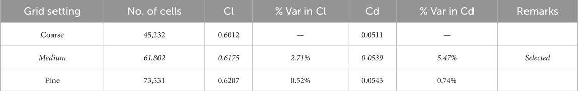
Table 1. Variation in predicted coefficients with different mesh setting.

The no-slip “wall” boundary condition was chosen for the airfoil, while the “velocity-inlet” was chosen for the inlet, and the “pressure-outlet” condition was chosen for the exit. Figure 2 shows the meshing constructed around the airfoils, with very fine meshing with inflation layers at the airfoil surface.

Figure 2

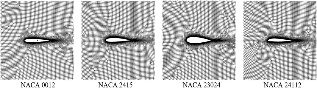
Figure 2. Unstructured mesh around the airfoils.

An aerodynamic dataset of 440 cases was obtained by numerical simulations on the airfoils at various flow conditions. The Mach number of the flow was kept constant in all cases, whereas a combination of ten different Reynolds numbers and eleven different angles of attack were simulated on all four airfoils to generate the dataset. Reynolds numbers (Re) were chosen from 0.5 to five million with an increment of 0.5 million in between, and angles of attack were chosen from 0° to 20° with an increment of 2° in between. Reynolds numbers in this range indicate the commencement of turbulence and transition to the completely turbulent boundary layer above the surface of the airfoil. The range is located in the mid-domain on the scale, indicating low-to-high Reynolds number [27]. Thus 110 cases were simulated on each airfoil, making a total 440 cases on all four airfoils combined. Note that the same aerodynamic dataset has also been used in our previous study on airfoil analysis using back-propagation neural networks [20]. However, this study extends the scope by building upon the prior dataset in a technically rigorous manner for implementing multiple SVM models under identical conditions, accentuating its applicability as a low-cost surrogate. New or additional simulations were considered needless at this point, as the existing dataset’s range sufficiently captures nonlinear aerodynamic regimes. Details of the numerically simulated flow conditions are tabulated in Table 2.

Table 2

Table 2. Details of flow conditions simulated.

For better visualization, the scatter plot of the numerically simulated flow conditions is also illustrated in Figure 3. It can be observed that similar flow conditions have been numerically simulated for all four NACA airfoils chosen for this paper to generate the required aerodynamic dataset. It should be noted that while the data splitting for training was done at random, there may not have been an equal amount of data points from each airfoil for the training.

Figure 3

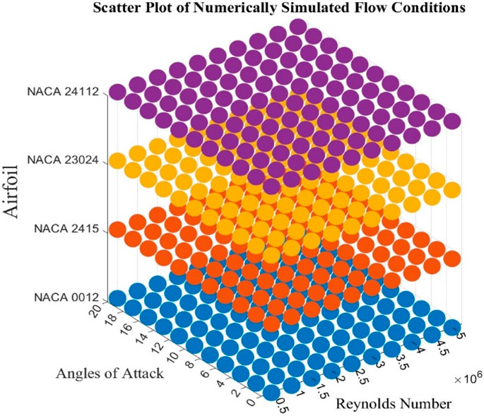
Figure 3. Scatter plot of numerically simulated flow conditions.

2.2 Support vector machines (SVMs)

This algorithm falls under the category of supervised machine learning techniques which help classify data into two groups [28]. This method involves identifying an optimal line, also known as a hyperplane, which splits data points to divide them into two groups, leaving the highest possible gap between them. It tries to find the line or plane that distinguishes the data points into the best possible groups or types. The points also called the vectors that are closest to it—referred to as the “maximum-margin hyperplane” — known as the “support vectors” [29]. SVMs convert the data into an upper-dimensional space using various methods (referred to as kernel functions), which simplifies the separation of the data points. This helps SVMs model complex associations between input and output variables. Due to the kernel functions, which enable them to handle both linear and nonlinear connections, SVMs are resilient against outliers, efficient for high-dimensional data, and adaptable. The linear kernel, quadratic kernel and cubic kernel, which are collectively known as polynomial kernels, and Gaussian kernels, also known as radial-basis functions (RBF) are among the frequently used kernels [30]. The efficacy of SVM largely hangs on the selection of kernel, the kernel’s parameters, and the soft margin parameter. The technique is chosen based on the data and expected relationship between them. Although SVMs are better at classification tasks, they can equally be used for regression tasks. The variant of SVM that predicts continuous values is called the Support Vector Regression (SVR) [31]. Its design is similar to SVM, as seen in Figure 4.

Figure 4

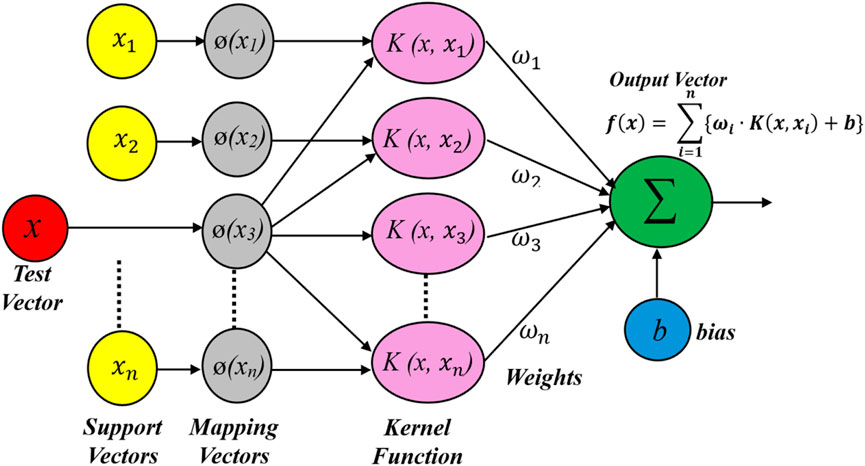
Figure 4. Generalized design of a SVMs.

The four primary phases in the SVM’s overall framework are as follows.

a. Pre-processing of data, whereby the input variables are suitably standardized to guarantee a well-adjusted input to the SVM model.

b. Selection of Kernel, where a suitable kernel function is selected according to the properties of the data.

c. Training the system to identify the best hyperplane for the given scenario.

d. Applying suitable assessment measures to assess the model’s performance.

The pseudo algorithm as per the above general framework for Support Vector Regression (SVR) as implemented in this work is described below in seven broad steps. It is to be noted that the algorithm’s convergence criteria can be customized by adjusting the weight updates and iteration count, which serve as a stopping condition.

a. Data Preparation: Define the input vector set $x_i$ and corresponding output labels $y_i$.

b. Kernel Selection: Choose a suitable kernel, $K\left(x,x_i\right)$ for converting inputs into upper-dimensional space.

c. Initialization: Set initial parameters: regularization factor C, kernel K, and tolerance margin ε.

d. Model Optimization: Minimize the objective function using (Equation 1) with the training data $\left(x_i,y_i\right)$ to determine optimal SVR model parameters.

$\left.\mathit{min}\frac{1}{2}{‖\omega ‖}^2+C\frac{1}{n}{\displaystyle \sum _{i=1}^n}\left\{y_i\right.-\left(\omega ·x_i+b\right)-\epsilon \right\}(1)$

e. Prediction: Use optimized SVR model parameters to predict output values for new input vectors.

f. Output Calculation: For a new input vector x, calculate the predicted output $\widehat{y}$ using (Equation 2).

$\widehat{y}=\omega ·x+b(2)$

g. Regression Function Approximation: Approximate the regression function using (Equation 3).

$f\left(x\right)={\displaystyle \sum _{i=1}^n}\left\{{\omega }_i·K\left(x,x_i\right)\left.+b\right\}\right.(3)$

Here, $f\left(x\right)\to$ it denotes the set of output vectors,$K\to$ it denotes the kernel function,${\omega }_i\to$ it denotes the weight vector,$b\to$ it denotes the bias term

h.Kernel Functions: Use (Equation 4) for linear, (Equation 5), for polynomial or (Equation 6) for RBF kernel to get the SVM parameters.

$K\left(x,x_i\right)=x.x_i(4)$

$K\left(x,x_i\right)={\left(\gamma .x.x_i+c\right)}^d(5)$

Here, $\gamma \to$ scaling factor,

$c\to$ offset constant,

$d\to$ degree of polynomial.

$K\left(x,x_i\right)=\exp \left.\left\{\gamma \right.{‖x-x_i‖}^2\right\},\gamma >0(6)$

Here, $\gamma \to$ scaling factor,

${‖x-x_i‖}^2\to \text{Euclidean\hspace{0.17em}distance\hspace{0.17em}}\mathrm{b}/\mathrm{w}x\&x_i$

2.3 Predictive model

The rudimentary model to predict aerodynamic coefficients with SVM as used in this present paper is shown in Figure 5. The SVM model can be taken as a black box that takes certain inputs and produces certain outputs. In the case of current work, the inputs are the four input features, i.e., airfoil nomenclature (noun), Mach (Ma) and Reynolds numbers (Re), and airfoil’s angle of attack (AoA), and the outputs are the drag coefficient (C_d) and lift coefficient (C_l).

Figure 5

Figure 5. Svm predictive model.

2.4 Data processing, model training and implementation

Figure 6 depicts the fundamental flowchart for the suggested methodology. Initially, the required aerodynamic dataset was created through numerical simulations on four airfoils at various flow conditions in Ansys Fluent.

Figure 6

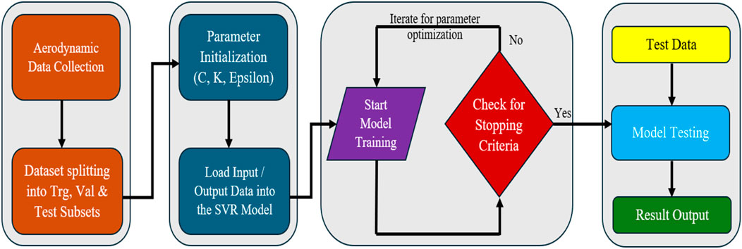
Figure 6. Flowchart for SVM implementation.

Prior to model training, data preprocessing was conducted on the dataset to ensure its integrity. The dataset was initially examined manually for any missing values and outliers to ensure data integrity. It is important to note that because of the small dataset (440 data points only), no missing values or outliers were found; therefore, automated outlier detection or data imputation was not needed. Moreover, considering the controlled nature of the numerical simulations and the small dataset size, no extra filtering or smoothing was performed on the data. Normalization was also considered unnecessary because the aerodynamic coefficients varied consistently.

Feature selection is another important element of data preprocessing. In order to estimate the aerodynamic coefficients, four important parameters, including the angle of attack (AoA), Mach (Ma), Reynolds number (Re) and the airfoil name were selected as the input features. The airfoil name, being a categorical feature, was encoded numerically using a label encoding scheme. Each of the four airfoils was assigned to a unique integer such as NACA 0012 as 1, NACA 2415 as 2, NACA 23024 as 3 and NACA 24112 as 4. This allowed the airfoil identifier to be used as an input feature without disrupting numerical processing. The outputs or the targets were the drag coefficient (C_d) and lift coefficient (C_l).

The dataset was then split into three subsets: training, validation, and testing. The dataset was randomly split into 70% for training, i.e., around 308 data points were chosen randomly for training, and 15% each, i.e., 66 data points each were chosen for testing and validation purposes, respectively. After which the kernel functions were selected, and the model was initialized with random values. Subsequently, the training dataset was provided to the SVM model to start the training. The training terminated on attaining the predetermined stopping conditions. When the validation error was reduced to its smallest value, i.e., on attaining the best validation performance was the stopping criterion intended to be reached. The trained model was then assessed with the testing data subset.

The SVM models were trained by utilizing the “Regression-Learner” application available in MATLAB R2023b for forecasting the aerodynamic coefficients of airfoils. The regression learner can train various regression models to predict data utilizing supervised approaches of machine learning [32]. To predict the aerodynamic coefficient in the current work, six different forms of SVMs including linear, quadratic, cubic, fine, medium, and coarse models have been used. The kernel functions and kernel scaling that were employed for training distinguish the models from one another.

The default settings of hyperparameters were kept for the support vector machines used in this work to simplify the model, ensure consistency and avoid model-specific bias during evaluation. This approach enables rapid deployment of the existing model without extensive manual tuning. The selected default settings include automatic kernel scaling, regularization parameters, and epsilon-insensitive loss parameters. The standard by which to select the box constraints was also set to automatic. This allowed a fair comparison of kernel efficacy. It is to be noted here that no grid or random search tuning was employed during this study. Hyperparameter optimization using different techniques like Bayesian optimization etc. May be potentially used in future studies which can enhance the model’s performance. The selected hyperparameters as per the default settings of the MATLAB’s Regression-Learner App are summarized in Table 3.

Table 3

Table 3. Hyper parameters of SVM models.

2.5 Performance assessment criterions

The performance of the SVM models after training has been evaluated using the most widely used statistical performance gauges. These are, namely, the root mean squared error denoted as RMSE, the Mean Absolute Error denoted as MAE, and the Pearsons Correlation Coefficients denoted as R which are defined as below.

2.5.1 Root mean squared error (RMSE)

RMSE is defined by the rooted difference between the forecasted and the actual goal. Square root ensures that it is of the same order as the predicted values. The accuracy of the model is inversely proportional to the RMSE; that is, a lesser value of the RMSE represents better accuracy of the model. Ideally, it should approach zero. Mathematically, it is defined by (Equation 7).

$RMSE=\sqrt{\frac{1}{n}{\displaystyle \sum _{i=1}^n}{\left|P_i-M_i\right|}^2}(7)$

Here, $P_i\to$ forecasted value

$M_i\to$ actual goal

2.5.2 Mean absolute error (MAE)

MAE is used to evaluate the accuracy of regression models for which the error direction is not critical. It is determined by calculating the mean absolute variance between the forecasted and the actual goal. The lower value of the MAE represents better model performance. It is important to compare the MAE to the scale of the target variable. Ideally, it should also be zero. Mathematically, it is defined by (Equation 8).

$MAE=\frac{{\displaystyle {\sum }_{i=1}^n}\left|P_i-M_i\right|}{n}(8)$

Here, $P_i\to$ forecasted value

$M_i\to$ actual goal

2.5.3 Pearson’s correlation coefficient (R)

“R” is an important statistical metric that shows the association between the forecasted and the actual goal. It always falls between $-1$ and $+1$. The performance of a model is ideal if the absolute value of R is equivalent to or remarkably close to +1. Mathematically, it is defined by (Equation 9).

$R=\sqrt{1-\frac{\sum {\left(M_i-P_i\right)}^2}{\sum {\left(M_i-{\overline{M}}_l\right)}^2}}(9)$

Here, $n\to$ total no. of data points

$P_i\to$ forecasted value

$M_i\to$ actual goal

$\overline{M_l}\to$ mean of all measured values

3 Results and discussions

In this work, our primary focus is to conduct a detailed evaluation of six SVM variants for predicting lift and drag coefficients of four NACA airfoils using a consistent CFD dataset and protocol. While other machine-learning architectures such as BPNNs, CNNs, and LSTMs have been reported in the literature, they typically differ in input representation, target variables, preprocessing steps, and evaluation metrics, making direct numerical comparison to the present results inappropriate without retraining under identical conditions. To maintain methodological consistency and avoid misleading conclusions, this study limits its scope to SVM-based methods evaluated in a uniform framework. Each model studied in this work was trained independently for predicting the aerodynamic drag coefficient and lift coefficient on a numerically generated dataset of 440 cases. Table 4 summarizes the vital performance evaluation metrics of RMSE, MAE, and R acquired during validation for each SVM model in forecasting drag and lift coefficients.

Table 4

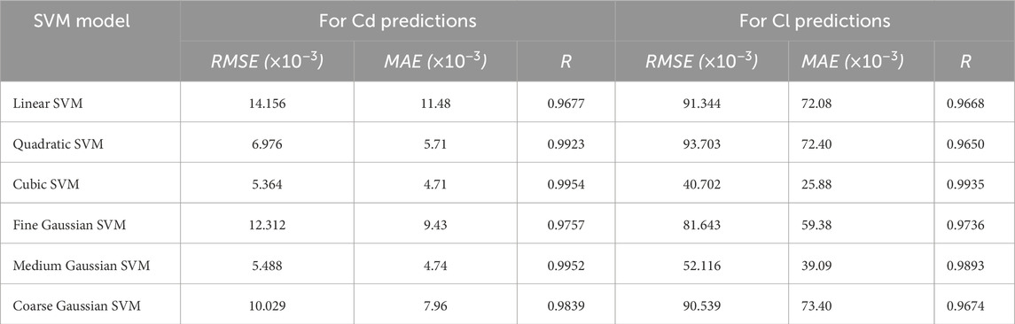
Table 4. Results summary for different SVM models.

From Table 4, it can be noted that the cubic SVM model has yielded the best outcomes in terms of the performance evaluation metrics by achieving the best values for RMSE, MAE, and R for estimating both the aerodynamic coefficients. The RMSE value achieved by cubic SVM for estimating the drag coefficient was 5.364 $\times$ 10⁻³ and the lift coefficient was 40.702 $\times$ 10⁻³, along with correlation coefficients of 0.9954 and 0.9935, respectively. These values depict a strong correlation between the forecasted and actual responses, indicating the effectiveness of the cubic kernel in modeling the nonlinear correlations between aerodynamic variables.

The effectiveness of the cubic SVM is attributed to its ability to distinguish complex flow phenomena like flow separation and abrupt lift changes at medium to high angles of attack. The superior performance can be explained by considering both the physics of the aerodynamic prediction task and the mathematical properties of the kernel. The relation between flow characteristics (Reynolds number, Mach number, angle of attack) and aerodynamic coefficients is naturally smooth but may exhibit nonlinearities due to complex flow phenomena like flow separation, pressure distribution changes, and viscous effects. A cubic polynomial kernel effectively captures nonlinearities due to its ability to integrate interactions up to the third order, without the limited flexibility of linear/quadratic kernels or the excessive locality of narrow Gaussian kernels. The CFD dataset used in this study is continuous and free from measurement noise, allowing the global basis functions of the cubic kernel to exploit the smoothness of the aerodynamic response surface. These combined factors explain the cubic kernel’s ability to achieve a favorable trade-off between model complexity and generalization accuracy.

The medium Gaussian SVM model has also produced results remarkably close to the cubic SVM model in predicting both the aerodynamic coefficients with RMSE values of 5.488 × 10^-3 and 52.116 × 10^-3 for drag and lift coefficients, respectively. It can be said that due to the inherent smoothness of the radial basis function kernel of the medium Gaussian SVM, it was able to learn the localized patterns in variation without the risk of overfitting.

On the other hand, the linear and quadratic SVM had the worst performance for drag coefficient and lift coefficient with RMSE values of 14.156 × 10^-3 and 93.703 × 10^-3, respectively, while correlation coefficient values remained above 0.9650. The drop in performance by the linear and quadratic kernels can be attributed to their limitations in modeling the complex flow behaviors like flow separation and abrupt lift changes, which are nonlinear in nature.

On deeper analysis of the results, another important aspect can be observed here: all SVM models studied predicted both the aerodynamic coefficients with good accuracy, but their performance is almost 7 to 8 times better in predicting the coefficient of drag as compared to the coefficient of lift. In all cases, the RMSE and MAE values remained lower for prediction of drag coefficient as compared to lift coefficient.

A possible explanation for this phenomenon is the difference in flow characteristics when producing drag and lift. Drag varies smoothly with respect to changes in Reynolds number, flow speed and/or angle of attack due to its inherent dependence on pressure and skin friction drag along the airfoil surface, making it easier for the machine learning model to remember and generalize it. Whereas the lift is dependent upon the pressure difference between the upper and lower surfaces of the airfoil, which is highly sensitive to Reynolds number, flow speed and/or angle of attack. As the angle of attack approaches the stall region, the adverse pressure gradient intensifies, causing the laminar boundary layer to transition earlier to turbulence and, in some cases, to separate from the surface entirely. This separation drastically alters the surface pressure distribution, leading to sharp drops in lift and significant variability even with small perturbations in operating conditions. Additionally, vortex shedding and unsteady wake interactions near stall introduce temporal fluctuations absent in the relatively steady drag trends. Resultantly, while the mapping from inputs to Cd is relatively smooth and single-regime, the mapping for Cl frequently spans multiple aerodynamic regimes (attached flow, transitional flow, separated flow), introducing nonlinearities and increasing functional complexity, making approximation more difficult for a single machine learning model.

The RMSE values obtained for each SVM model for predicting the coefficient of drag and coefficient of lift are shown separately in Figure 7. Notably, the cubic SVM consistently outperformed other models in both cases with RMSE values of 5.364 $\times$ 10⁻³ and 40.702 $\times$ 10⁻³ for prediction of coefficients of drag and lift, respectively.

Figure 7

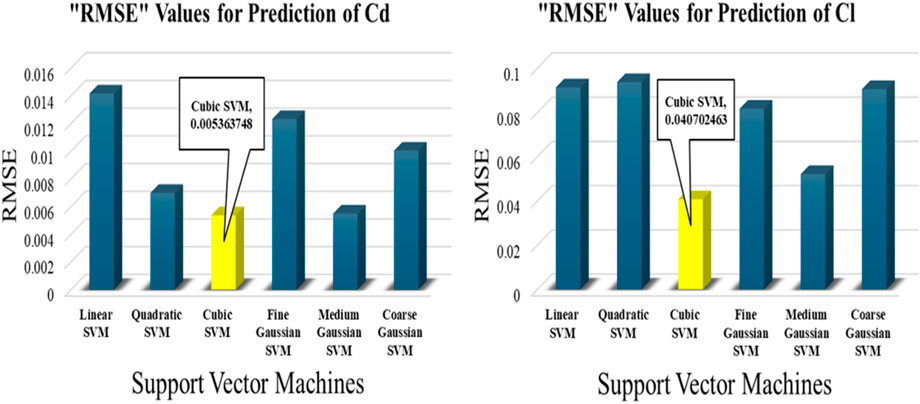
Figure 7. RMSE plots for SVM models for Predicting Cd and Cl.

Table 4 further indicates that the MAE values follow a trend consistent with RSME for all the SVM models, reinforcing the superiority of cubic SVM across all metrics. This has been depicted in Figure 8, where the plot of MAE values for each SVM model has been provided separately for predictions of drag coefficient as well as lift coefficient. The best MAE value achieved by Cubic SVM for estimating the drag coefficient was 4.71 $\times$ 10⁻³ and the lift coefficient was 25.88 $\times$ 10⁻³, respectively.

Figure 8

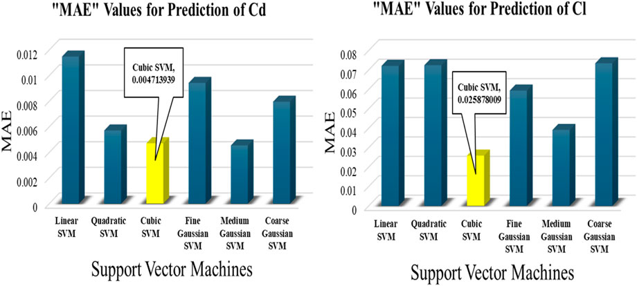
Figure 8. MAE plots for SVM models for Predicting Cd and Cl.

Table 4 also shows that the value of “R” was extremely near to +1 in all the scenarios, representing the accuracy of the estimated aerodynamic coefficients. Best values, however, were again achieved by the cubic SVM model for both aerodynamic coefficient predictions.

The performance of all the SVM models to estimate the drag coefficient and lift coefficient are depicted through the regression charts given in Figures 9, 10, respectively. These regression plots further validate the conclusions. Each subplot shows a comparison between the predicted and true responses, with the corresponding R values representing the model’s ability to fit. The graph illustrates a strong association between the estimated and actual goal; furthermore, most of the data points are on or very close to the regression (ideal) line.

Figure 9

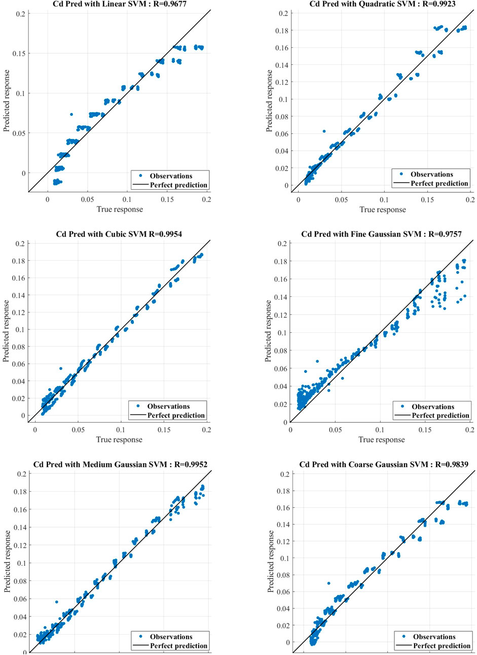
Figure 9. Regression Charts for all SVM model for Predicting Coefficient of Drag Cd.

Figure 10

Figure 10. Regression Charts for all SVM model for Predicting Coefficient of Lift Cl.

Figure 9 represents the regression plots of predicted versus actual drag coefficients for all six SVM models. The performance of each model can be measured based on the data clustering around the regression (ideal) line and the related R values. It can be clearly seen that the cubic SVM and medium Gaussian SVM are closely clustered around the ideal fit line with nominal scattering, with R-values exceeding 0.99. This depicts excellent correlation between the predicted and actual values, reflecting the model’s ability to capture complex aerodynamic relationships with minimal variance. The quadratic and fine Gaussian SVM models also provided reasonably good performance, though with slightly more spread in the residual values around the regression line, indicating lesser performance.

In contrast, the linear SVM and coarse Gaussian SVM models have shown broader scatter, especially at the lower and higher ranges of drag coefficients, where it underfitted the ideal line. This particular behavior is attributed to their limited capacity to model nonlinear variations due to skin-friction and pressure drag across varying Reynolds numbers and angles of attack. This supports the earlier conclusion that nonlinear kernels, particularly cubic and medium Gaussian, are better suited for modeling drag behavior. It is to be noted that even the weaker models like linear SVM have achieved R-values above 0.96, indicating reasonable accuracy while predicting drag coefficients within a constrained domain. However, their reduced accuracy especially at low and high ranges indicates limitations in capturing detailed drag behavior near flow transition or flow separation conditions.

Figure 10 illustrates the regression plots of predicted versus actual lift coefficients for all six SVM models. Here the performance differences between the SVM models are more pronounced as compared to the drag coefficients prediction. For lift coefficients prediction as well, the cubic SVM has outperformed other models, with a near ideal scattering of data points around the regression (ideal) line, indicating its capability of modeling nonlinear aerodynamic lift behavior. The medium Gaussian SVM has also performed well, although with a slightly more scattering of datapoints especially at higher values of lift coefficients. This shows a slight decrease in performance at higher angles of attack where flow separation and stall effects come in to play. The fine Gaussian SVM has produced a larger variance and a noticeable underestimation in certain regions, possible due to overfitting on localized features without capturing global patterns effectively.

The linear and quadratic SVMs have shown the weakest performance for prediction of lift coefficients. These have produced the largest spread of datapoints further from the ideal fit line at both low and high lift regions. This behavior depicts their inadequacy in handling the complexity of relationship between the input parameters owing to nonlinearities inherent in lift generation, especially at transitional stages. Overall, the Figure 10 depicts that lift coefficients prediction is inherently more challenging than drag coefficients prediction due to its dependency on more complex fluid dynamics phenomena.

The regression plots of drag coefficients and lift coefficients prediction have validated the data presented in Table 4. They have also shown the superiority of nonlinear kernels including the cubic and medium Gaussian SVMs in capturing aerodynamic complexities more efficiently.

The performance ranking of different variants of SVMs is supported by multiple performance measuring metrics (RMSE, MAE, and Pearson’s R) and by consistent patterns observed in residual plots. As these indicators agree and the effect sizes are clear, formal hypothesis testing was considered unnecessary. Additionally, classical statistical tests assume that prediction errors are independent and have a uniform spread across all operating conditions, which is not strictly satisfied in the aerodynamic dataset used in this work due to its structured nature, and could therefore yield misleading p-values. The combination of several metrics and regression plots is considered sufficient to demonstrate the robustness of the conclusions.

4 Limitations and considerations

Despite the fact that the cubic and medium Gaussian SVM models have fairly predicted the aerodynamic coefficients, it is to be noted that there are some limitations associated with the current study. First of all, the performance of the SVM models are purely dependent upon the quality and quantity of the training dataset. Machine learning techniques require large amount of datasets for proper training, however, SVM models have been trained only on a dataset of 440 simulation cases in this study, which may be a potential limitation for the model’s performance. Moreover, the investigated SVM model’s performance have been assessed on a limited subset of airfoil (only NACA 4- and 5- digit series) configurations under a limited flow condition to maintain a controlled geometric parameter space and ensure consistent CFD meshing and boundary conditions across all cases. While this restriction enables fair benchmarking of SVM kernels, it does not capture the full geometric diversity of airfoils. Therefore, their performance may not be directly generalize to other situations and datasets with the same level of accuracy without retraining.

Secondly, in comparison to the traditional CFD techniques, the SVM model operates as black-box model offering limited physical interpretability of what’s happening inside the model. Lastly, to simplify the model implementation, default values of the hyperparameters have been used during training, which may become a limitation in reaching optimal performance of the models. In order to address these limitations, training the models on a large and more diversified dataset obtained from further CFD simulations of different types of airfoils under numerous settings, hyperparameter optimization using various techniques like Bayesian optimization etc., and integration with physics-based constraints may help to increase the reliability of the results. A valuable extension of this research would be to retrain representative deep learning and ensemble models on the same dataset and evaluation protocol used here. Such an experiment would allow a direct, fair, and quantitative comparison between SVMs and other state-of-the-art techniques, providing further insight into the trade-offs between accuracy, computational efficiency, and model interpretability.

5 Conclusion

In this study, we assessed the performance of six distinct Support Vector Machine models in predicting the aerodynamic coefficients of drag and lift under a wide range of flow conditions for four different NACA airfoils. In this regard, a dataset of 440 cases generated through numerical simulations was used to train and evaluate the models. The cubic SVM exhibited the best predictive performance among all the tested models, demonstrating the lowest RMSE of 5.364 × 10^-3 for drag coefficient and 40.702 × 10^-3 for lift coefficient. Correlation coefficient values higher than 0.995 were also achieved in each case, indicating a very high correlation between tested and predicted data. The performance of the medium Gaussian SVM was also comparable to the cubic SVM model, signifying its capability to model the complex and nonlinear aerodynamic behavior. On the other hand, the linear SVM and quadratic SVM had the worst performance for drag coefficient and lift coefficient with RMSE values of 14.156 × 10^-3 and 93.703 × 10^-3, respectively, while correlation coefficient values remained above 0.9650.

Overall, the SVM models proved effective in aerodynamic modeling of airfoil aerodynamics under varying angles of attack and Reynolds numbers. The results indicate that adequately tuned machine learning models, especially the nonlinear SVM models, can act as surrogates for costly numerical schemes without a substantial compromise in accuracy. However, it is important to highlight that the results are based on the specific dataset used in this study and may not be applicable globally in the present form. Additionally, the models were trained using default MATLAB hyperparameters to maintain fairness and simplicity across comparisons. The findings of this study can be further expanded by including additional airfoils and more flow regimes to get larger datasets. Moreover, hyperparameters tuning to get potentially better performance of the SVM models may be done through optimization schemes and integration with other machine learning algorithms in future studies to further enhance the predictive capabilities and generalization of these techniques for broader aerodynamic applications.

Data availability statement

The raw data supporting the conclusions of this article will be made available by the authors, without undue reservation.

Author contributions

SA: Conceptualization, Data curation, Formal Analysis, Methodology, Software, Visualization, Writing – original draft, Writing – review and editing. KK: Conceptualization, Formal Analysis, Methodology, Resources, Supervision, Validation, Writing – review and editing. TA: Conceptualization, Data curation, Methodology, Project administration, Supervision, Writing – review and editing. BL: Methodology, Formal Analysis, Funding acquisition, Resources, Validation, Writing – review and editing. NA: Methodology, Formal Analysis, Funding acquisition, Resources, Visualization, Writing – review and editing.

Funding

The author(s) declare that financial support was received for the research and/or publication of this article. This work was supported and funded by the Deanship of Scientific Research at Imam Mohammad Ibn Saud Islamic University (IMSIU) (grant number IMSIU-DDRSP2503).

Conflict of interest

The authors declare that the research was conducted in the absence of any commercial or financial relationships that could be construed as a potential conflict of interest.

Generative AI statement

The author(s) declare that no Generative AI was used in the creation of this manuscript.

Any alternative text (alt text) provided alongside figures in this article has been generated by Frontiers with the support of artificial intelligence and reasonable efforts have been made to ensure accuracy, including review by the authors wherever possible. If you identify any issues, please contact us.

Publisher’s note

All claims expressed in this article are solely those of the authors and do not necessarily represent those of their affiliated organizations, or those of the publisher, the editors and the reviewers. Any product that may be evaluated in this article, or claim that may be made by its manufacturer, is not guaranteed or endorsed by the publisher.

References

1. Rizzi A, Oppelstrup J. Airfoil design considerations. Aircraft aerodynamic design with computational software. Cambridge: Cambridge University Press (2021). p. 272–99. doi:10.1017/9781139094672.010

CrossRef Full Text | Google Scholar

2. Bhatnagar S, Afshar Y, Pan S, Duraisamy K, Kaushik S. Prediction of aerodynamic flow fields using convolutional neural networks. Comput Mech (2019) 64(2):525–45. doi:10.1007/s00466-019-01740-0

CrossRef Full Text | Google Scholar

3. Liu T. Evolutionary understanding of airfoil lift. Adv Aerodyn (2021) 3(1):37. doi:10.1186/s42774-021-00089-4

CrossRef Full Text | Google Scholar

4. Juvinel JMDE, Roa DPP, Schaerer CE. Structural and shape optimization in aerodynamic airfoil performance: a literature review. Preprints (2023) 12:2023070807. doi:10.20944/preprints202307.0807.v1

CrossRef Full Text | Google Scholar

5. Gupta SB, Tyagi RK, Gairola A. A review on evolution of airfoils and their characteristics in last three centuries part-2: evolution of airfoils and their characteristics after 1930 and NACA series with characteristics of subsonic and high subsonic airfoils. AIP Conf. Proc. (2022) 2597(1):070001. doi:10.1063/5.0117414

CrossRef Full Text | Google Scholar

6. Van Messem A (2020). Support vector machines: a robust prediction method with applications in bioinformatics. ASR Srinivasa Rao, and CR Rao, Eds. in Principles and methods for data science vol. 43 Elsevier, pp. 391–466. doi:10.1016/bs.host.2019.08.003

CrossRef Full Text | Google Scholar

7. Duraisamy K, Iaccarino G, Xiao H. Turbulence modeling in the age of data. Annu Rev Fluid Mech (2019) 51(1):357–77. doi:10.1146/annurev-fluid-010518-040547

CrossRef Full Text | Google Scholar

8. Li J, Du X, Martins JRRA. Machine learning in aerodynamic shape optimization. Prog Aerosp Sci (2022) 134:100849. doi:10.1016/j.paerosci.2022.100849

CrossRef Full Text | Google Scholar

9. Le Clainche S, Ferrer E, Gibson S, Cross E, Parente A, Vinuesa R. Improving aircraft performance using machine learning: a review. Aerosp Sci Technol (2023) 138:108354. doi:10.1016/j.ast.2023.108354

CrossRef Full Text | Google Scholar

10. Kaya M. A CFD based application of support vector regression to determine the optimum smooth twist for wind turbine blades. Sustainability (2019) 11(16):4502. doi:10.3390/su11164502

CrossRef Full Text | Google Scholar

11. Zeng J, Qiao W. Short-term solar power prediction using a support vector machine. Renew Energy (2013) 52:118–27. doi:10.1016/j.renene.2012.10.009

CrossRef Full Text | Google Scholar

12. Primadusi U, Cahyadi AI, Wahyunggoro O. The comparison of RBF NN and BPNN for SOC estimation of LiFePO4 battery. In: PROCEEDINGS OF THE 12TH INTERNATIONAL CONFERENCE ON SYNCHROTRON RADIATION INSTRUMENTATION – SRI2015, 1741. New York, NY USA (2016). 090010. doi:10.1063/1.4958528

CrossRef Full Text | Google Scholar

13. Herulambang W, Hamidah MN, Setyatama F. Comparison of SVM and BPNN methods in the classification of batik patterns based on color histograms and invariant moments. In: 2020 international conference on smart Technology and applications (ICoSTA), surabaya, Indonesia. IEEE (2020). p. 1–4. doi:10.1109/ICoSTA48221.2020.1570615583

CrossRef Full Text | Google Scholar

14. Najwa Mohd Rizal N, Hayder G, Mnzool M, Elnaim BME, Mohammed AOY, Khayyat MM. Comparison between regression models, support vector machine (SVM), and artificial neural network (ANN) in river water quality prediction. Processes (2022) 10(8):1652. doi:10.3390/pr10081652

CrossRef Full Text | Google Scholar

15. Kostas KV, Manousaridou M. Machine-learning-enabled foil design assistant. J Mar Sci Eng (2023) 11:1470. doi:10.3390/jmse11071470

CrossRef Full Text | Google Scholar

16. Andrés-Pérez E, Paulete-Periáñez C. On the application of surrogate regression models for aerodynamic coefficient prediction. Complex Intell Syst (2021) 7(4):1991–2021. doi:10.1007/s40747-021-00307-y

CrossRef Full Text | Google Scholar

17. Ahmed S, Kamal K, Ratlamwala TAH. Relative assessment of selected machine learning techniques for predicting aerodynamic coefficients of airfoil. Iran J Sci Technol Trans Mech Eng (2024) 48:1917–35. doi:10.1007/s40997-023-00748-5

CrossRef Full Text | Google Scholar

18. Yan L, Chang X, Wang N, Zhang L, Liu W, Deng X. Comparison of machine learning and classic methods on aerodynamic modeling and control law design for a pitching airfoil. Int J Aerosp Eng (2024) 2024(1):5535800. doi:10.1155/2024/5535800

CrossRef Full Text | Google Scholar

19. Özgören AC, Acar DA, Kamrak R, Eriş GM, Özdemir Y, Uzol NS, et al. Machine learning based predictions of airfoil aerodynamic coefficients for Reynolds number extrapolations. J Phys Conf Ser (2024) 2767(2):022049. doi:10.1088/1742-6596/2767/2/022049

CrossRef Full Text | Google Scholar

20. Ahmed S, Kamal K, Ratlamwala TAH, Mathavan S, Hussain G, Alkahtani M, et al. Aerodynamic analyses of airfoils using machine learning as an alternative to RANS simulation. Appl Sci (2022) 12(10):5194. doi:10.3390/app12105194

CrossRef Full Text | Google Scholar

21. Michos A, Bergeles G, Athanassiadis N. Aerodynamic characteristics of NACA 0012 airfoil in relation to wind generators. Wind Eng (1983) 7(4):247–62. Available online at: http://www.jstor.org/stable/43749000.

Google Scholar

22. Anil Kumar BS. Computational investigation of flow separation over naca 23024 airfoil at 6 million free stream Reynolds number. Int J Sci Technol Soc (2015) 3(6):315. doi:10.11648/j.ijsts.20150306.17

CrossRef Full Text | Google Scholar

23. Spalart P, Allmaras S. A one-equation turbulence model for aerodynamic flows. In: 30th aerospace sciences meeting and exhibit. Reno, NV, U.S.A.: American Institute of Aeronautics and Astronautics (1992). doi:10.2514/6.1992-439

CrossRef Full Text | Google Scholar

24. Ahmed S, Malik A, Parvez K. RANS predictions of junction flow with localized suction. In: 2018 IEEE International conference on aerospace electronics and remote sensing Technology (ICARES), Bali. IEEE (2018). p. 1–7. doi:10.1109/ICARES.2018.8547058

CrossRef Full Text | Google Scholar

25. F. Inc. FLUENT 6.3 user’s guide. USA: Fluent Inc. (2006).

Google Scholar

26. NACA. NACA 4 series airfoil generator. AeroToolbox (2024). Available online at: https://aerotoolbox.com/naca-4-series-airfoil-generator/ (Accessed: October 21, 2024).

Google Scholar

27. Wang S, Zhou Y, Alam MM, Yang H. Turbulent intensity and Reynolds number effects on an airfoil at low Reynolds numbers. Phys Fluids (2014) 26(11):115107. doi:10.1063/1.4901969

CrossRef Full Text | Google Scholar

28. Vapnik V, Golowich S, Smola A. Support vector method for function approximation, regression estimation and signal processing. In: Advances in neural information processing systems. MIT Press (1996). Available online at: https://proceedings.neurips.cc/paper/1996/hash/4f284803bd0966cc24fa8683a34afc6e-Abstract.html (Accessed: December 13, 2022).

Google Scholar

29. Zendehboudi A, Baseer MA, Saidur R. Application of support vector machine models for forecasting solar and wind energy resources: a review. J Clean Prod (2018) 199:272–85. doi:10.1016/j.jclepro.2018.07.164

CrossRef Full Text | Google Scholar

30. Raghavendra. N S, Deka PC. Support vector machine applications in the field of hydrology: a review. Appl Soft Comput (2014) 19:372–86. doi:10.1016/j.asoc.2014.02.002

CrossRef Full Text | Google Scholar

31. Hu H, Yu J, Song Y, Chen F. The application of support vector regression and mesh deformation technique in the optimization of transonic compressor design. Aerosp Sci Technol (2021) 112:106589. doi:10.1016/j.ast.2021.106589

CrossRef Full Text | Google Scholar

32. MATLAB. Choose regression model options - MATLAB and simulink (2024). Available online at: https://www.mathworks.com/help/stats/choose-regression-model-options.html#bvmpn_3-1 (Accessed May 02, 2024).

Google Scholar