Modeling opinion polarization: can we control public discourse?

Introduction: Public opinion dynamics shape societal discourse, with engagement levels influencing the balance between polarization and depolarization.

Methods: We present a compartmental model inspired by epidemiology to analyze opinion dissemination under external interventions. The model categorizes individuals into susceptible, exposed, positive, negative, and mixed-emotion communicators, with a time-dependent step function $u(t)$ modeling controlled engagement surges during a finite intervention period.

Results: Our analysis focuses specifically on the effects of temporary interventions rather than long-term system evolution. The results highlight engagement as a key control mechanism in shaping ideological stability.

Discussion: Real-world interventions, such as government-imposed access restrictions, demonstrate how targeted engagement shifts influence public discourse. This study provides a mathematical framework for understanding how external interventions drive opinion evolution and offers insights into managing polarization in digital and social environments.

1 Introduction

Opinion dynamics models provide a mathematical framework for understanding how individuals in a population form, spread, and modify their opinions over time. Traditionally studied in social sciences, the formation and evolution of opinions have increasingly attracted interest from researchers in physics, mathematics, and computer science [3]. A variety of works focuses on constructing mathematical models of opinion dynamics, using tools from statistical physics, network theory as well as computational modeling [1, 2, 14, 15, 17, 20, 26, 34].

Several well-known opinion models have been proposed to describe different mechanisms of opinion evolution. One of the foundational models in this field is the Deffuant-Weisbuch model, which describes how individuals adjust their opinions through pairwise interactions, with convergence occurring only if their initial opinions are close enough [6]. Similarly, the Hegselmann-Krause model assumes that individuals update their opinions based on a weighted average of those within a specified confidence threshold [13], capturing how opinion fragmentation and clustering arise from selective interactions. Expanding on these ideas, bounded confidence models [21] further explore the role of echo chambers in social networks, where individuals tend to reinforce their pre-existing beliefs by selectively interacting with like-minded peers.Other important frameworks include the voter model, which captures opinion shifts through random imitation of neighbors [29], and Ising-type models that represent opinion dynamics as binary-state systems influenced by local alignment and noise, drawing inspiration from statistical physics [29].

Beyond these foundational models, numerous alternative approaches have been developed, utilizing a wide range of modeling techniques. One widely used strategy is agent-based modeling (ABM), which allows for rich micro-level realism by simulating individuals as autonomous entities interacting based on heterogeneous rules [3, 19, 23, 28]. However, complex ABMs can be difficult to initialize and parameterize [30], are often criticized for lack of transparency and difficulty in evaluation [24], and may generate high-dimensional output that is hard to interpret [16].

Alongside these approaches, epidemic-inspired frameworks have also been widely used to study opinion spread, leveraging their ability to describe diffusion processes in a manner analogous to disease transmission [5, 12]. Studies proposed adaptations of Susceptible-Infected-Recovered (SIR) models to opinion spread, emphasizing similarities between rumor transmission and epidemic propagation [5, 32, 33, 35, 36]. Additionally, Susceptible-Exposed-Infected-Recovered (SEIR) models have also been used to capture the dynamics of opinion evolution, incorporating factors such as sentiment-driven interactions, decision-making processes, and multilingual opinion transfer [4, 8, 9, 22, 28, 37].

Building on this analytical advantage, we adopt and extend the recent compartmental framework introduced by Geng et al. [11], which is itself inspired by epidemic modeling structures. A key innovation in our study is the inclusion of a Mixed-Emotion Compartment $(I_m)$, designed to represent individuals who simultaneously engage with and disseminate both polarized viewpoints—an aspect not addressed in prior models. In many discussions, individuals express support and opposition simultaneously. The $I_m$ compartment captures this behavior by modeling agents who propagate both sides, offering a more realistic structure for multi-directional discourse. Its inclusion also enables more flexible equilibrium structures by mediating the dynamics between polarized groups.

In many socio-political and ideological debates, individuals rarely adhere strictly to a single stance; rather, they endorse some aspects of a discussion while opposing others. Classical models categorize individuals into predefined states—such as neutral, positive, or negative—but fail to capture those who actively engage in discourse while disseminating mixed sentiments. These individuals shape discussions in multiple directions rather than reinforcing a single stance, as seen in political debates, where people may support aspects of a reform while rejecting others. To address this, we introduce the Mixed-Emotion Compartment $(I_m)$, which allows individuals to simultaneously propagate multiple, sometimes contradictory, viewpoints. This feature enhances our model’s ability to reflect the complexity of public discourse, where individuals actively shape opinion evolution by amplifying, countering, or reshaping narratives.

The remainder of this paper is structured as follows: In Section 2, we introduce the mathematical model for online public opinion dynamics, establish the positivity and boundedness of solutions, and determine the equilibrium points. Section 3 presents the stability analysis, where we derive the basic reproduction number, analyze the local and global asymptotic properties of the equilibrium points, and illustrate the results. Finally, in Section 4, we discuss our findings in the context of real-world social media discourse and suggest possible extensions to the model.

2 Modeling online public opinion dynamics: positive, negative, and mixed emotions under media interventions

2.1 Mathematical model

To analyze the dynamics of opinion dissemination under media interventions, we propose a compartmental model inspired by epidemiological frameworks. The model classifies the population into five compartments, where $S$ (Susceptible Individuals), $E$ (Exposed Individuals), $I_p$ (Positive Communicators), $I_n$ (Negative Communicators), and $I_m$ (Mixed-Emotion Communicators) represent the number of netizens in each state. The terms “positive”, “negative”, and “mixed-emotion” communicators are used to represent individuals who actively express views in support of, against, or engaging with both sides of a topic. These labels do not imply internal affective states but rather the public orientation of the opinions being communicated.

The governing equations of our model, presented below, describe the dynamical transitions between opinion states, while the corresponding flow diagram (Figure 1) visually represents these transitions

$\begin{array}{cc}\hfill S^{\prime }& =u\left(t\right)-\lambda S\left(I_p+I_n+I_m\right)-{\mu }_{1}S,\hfill \\ \hfill E^{\prime }& =\lambda S\left(I_p+I_n+I_m\right)-\left({\alpha }_1+{\alpha }_2+{\alpha }_3\right)E-{\mu }_{2}E,\hfill \\ \hfill I_p^{\prime }& ={\alpha }_{1}E+\omega I_n{I}_p+{\delta }_1{I}_m-{\mu }_3{I}_p,\hfill \\ \hfill I_n^{\prime }& ={\alpha }_{2}E-\omega I_n{I}_p+{\delta }_2{I}_m-{\mu }_3{I}_n,\hfill \\ \hfill I_m^{\prime }& ={\alpha }_{3}E-\left({\delta }_1+{\delta }_2\right)I_m-{\mu }_3{I}_m.\hfill \end{array}(1)$

Figure 1

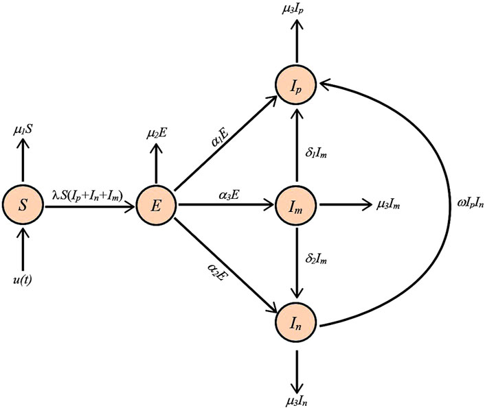
Figure 1. Flow diagram representing the opinion dynamics model in (Equation 1).

We assume that the disengagement rates for positive communicators $(I_p)$, negative communicators $(I_n)$, and mixed-emotion individuals $(I_m)$ are identical, denoted by ${\mu }_3$. This assumption is based on the idea that disengagement is primarily influenced by psychological fatigue, cognitive overload, and external platform mechanics rather than ideological stance. Empirical studies suggest that user disengagement from online discourse is often driven by information saturation rather than ideological conviction [18, 25, 27]. Furthermore, in many controlled environments—such as state-regulated media platforms or algorithmically moderated online spaces—users are subject to similar disengagement pressures, reinforcing our choice of a uniform ${\mu }_3$. While this study assumes a homogeneous disengagement rate, future work could explore the effects of asymmetrical disengagement rates, particularly in environments where ideological entrenchment plays a stronger role in sustained engagement.

In contrast, susceptible $(S)$ and exposed $(E)$ individuals have distinct disengagement rates $({\mu }_1,{\mu }_2)$, as their exit behaviors are fundamentally different. Political science research suggests that those who never engage in discourse disengage due to low motivation or cognitive effort [10]. Meanwhile, cognitive overload studies indicate that exposed individuals $(E)$, faced with conflicting opinions, are more prone to decision fatigue rather than ideological frustration [31]. By incorporating these distinctions, our model more accurately represents how individuals disengage at different stages of opinion formation.

In system (1), each derivative denotes the rate of change with respect to time $(t)$, which is modeled as a continuous and dimensionless variable. While the model does not assume a specific unit of time, it is designed to reflect the fast-paced nature of discourse evolution in digital environments. Depending on the application context, one unit of time can be interpreted as a few hours, a day, or a full cycle of social media engagement or news coverage. This flexible treatment allows the model to capture short-term fluctuations and longer-term opinion shifts within a unified analytical framework.

Here, $\lambda$ represents the probability of susceptible individuals transitioning into the exposed state after encountering active communicators, effectively becoming passive observers or ‘lurkers’. ${\alpha }_1$, ${\alpha }_2$ and ${\alpha }_3$ denote the probabilities of lurkers transitioning into different communicator states, specifically becoming positive, negative and mixed-emotion communicators, respectively. The transition rates ${\alpha }_1$, ${\alpha }_2$ and ${\alpha }_3$ are assumed to be constant, reflecting an internal predisposition of exposed individuals toward specific opinion states. These rates are not influenced by the current distribution of opinionated communicators in the system. $\omega$ refers to the probability of negative communicators shifting under positive influence, reflecting the interaction between opposing perspectives. Since $I_p$ and $I_n$ play structurally similar roles, the definition of $\omega$ as influencing either group remains a modeling choice, ensuring flexibility without affecting the fundamental structure or solution of the system.

The disengagement probabilities are given by ${\mu }_1$, ${\mu }_2$ and ${\mu }_3$, corresponding to different stages of engagement in the system. ${\mu }_1$ represents the probability of uninformed individuals disengaging from discourse entirely, while ${\mu }_2$ accounts for the probability of exposed individuals exiting the discussion before forming an opinion. Finally, ${\mu }_3$ denotes the probability of active communicators ($I_p$, $I_n$, $I_m$) disengaging, ceasing to contribute to opinion formation. Here, ${\delta }_1$ and ${\delta }_2$ represent the rate at which mixed-emotion individuals transition into positive and negative communicators, respectively. The inclusion of $I_m$ introduces a dynamic mediator that indirectly affects the balance between $I_p$ and $I_n$, allowing for more complex trajectories and equilibrium behavior than in traditional SEIR-type opinion models.

In our model, the influx of new individuals into the susceptible population is represented by the function $u(t)$, defined as

$u\left(t\right)=\left\{\begin{array}{cc}0,\hfill & \text{if\hspace{0.17em}}t<t_{\text{int}}\hfill \\ A,\hfill & \text{if\hspace{0.17em}}{t}_{\text{int}}\le t\le t_{\text{int}}+T_{\text{int}}\hfill \\ 0,\hfill & \text{if\hspace{0.17em}}t>t_{\text{int}}+T_{\text{int}}\hfill \end{array}\right..$

Here, $t_{\mathit{int}}$ denotes the initiation time of the intervention, $T_{\mathit{int}}$ represents its duration, and $A$ refers to the total number of new individuals entering the susceptible class during the intervention period. This piecewise definition allows us to model scenarios where external agents, such as governments or organizations, introduce surges of new participants into the discourse at strategically chosen times. By incorporating this time-dependent function, our model captures the transient and often abrupt changes observed in public opinion dynamics, providing a nuanced understanding of how targeted interventions influence the spread and evolution of opinions over time. In this study, we focus specifically on the time interval where $A$ is active, analyzing the effects of the intervention period. In our simulations, we focus on the case where $u(t)=A$ is constant, corresponding to a regime of sustained baseline engagement, in order to analyze the steady-state behavior of the system.

Engagement surges often arise from external factors such as major news events, viral media cycles, or coordinated platform-wide promotions. These triggers can cause abrupt increases in user participation, temporarily altering the trajectory of public discourse. Our model captures such surges through a time-dependent influx function, allowing for the analysis of how transient or sustained engagement influences long-term opinion dynamics.

2.2 Positivity and boundedness

A fundamental requirement in modeling such systems is ensuring that all state variables remain non-negative and bounded over time. This guarantees that the solutions remain physically meaningful, as negative values would not correspond to realistic interpretations of population sizes. The following theorem demonstrates that the total population remains constrained within a positively invariant region.

Theorem 1. Let $\mu$ denote the minimum of the coefficients ${\mu }_1$, ${\mu }_2$ and ${\mu }_3$. Then, the closed region

$\mathrm{\Omega }=\left\{\left(S,E,I_p,I_n,I_m\right)\in {\mathcal{R}}_{+}^5|S+E+I_p+I_n+I_m\le A/\mu \right\}$

is positively invariant set for the model given in (1).

Proof. To analyze the behavior of the system in (Equation 1), we sum the equations and define the total population as $N(t)=S(t)+E(t)+I_p(t)+I_n(t)+I_m(t)$, resulting in

$N^{\prime }\left(t\right)=S^{\prime }\left(t\right)+E^{\prime }\left(t\right)+I_p^{\prime }\left(t\right)+I_n^{\prime }\left(t\right)+I_m^{\prime }\left(t\right).$

By introducing $\mu =\text{min}\{{\mu }_1,{\mu }_2,{\mu }_3\}$, we derive the inequality

$N^{\prime }\left(t\right)\le A-\mu N\left(t\right),$

which clearly indicates that $N^{\prime }(t)$ becomes negative whenever $N(t)>A/\mu$.

Solving this inequality leads to the conclusion that

$N\left(t\right)\le \frac{A}{\mu }+e^{-\mu t}\left(N\left(0\right)-\frac{A}{\mu }\right),$

providing an upper bound for the total population as

$\underset{t\to \infty }{\lim }N\left(t\right)=\frac{A}{\mu }.$

Furthermore, for $(S,E,I_p,I_n,I_m)\in {\mathcal{R}}_{+}^5$, the following holds

$S^{\prime }{{|}_{S=0}=A>0,E^{\prime }|}_{E=0}=\lambda S\left(I_p+I_n+I_m\right)\ge 0,I_p^{\prime }{|}_{I_p=0}={\alpha }_{1}E+{\delta }_1{I}_m\ge 0,$

$I_n^{\prime }{|}_{I_n=0}={\alpha }_{2}E+{\delta }_2{I}_m\ge 0,I_m^{\prime }{|}_{I_m=0}={\alpha }_{3}E\ge 0.$

Therefore, $\mathrm{\Omega }$ constitutes a positively invariant set for the model (1), guaranteeing that no solution trajectory can leave through the boundary of $\mathrm{\Omega }$.

2.3 Equlibrium points

Analyzing the equilibrium points of the system provides insight into its long-term behavior. Equilibrium states correspond to points where the system remains unchanged over time, meaning all derivatives are set to zero. By solving the resulting algebraic equations, we can determine steady-state solutions that describe possible stable configurations of the system.

Solving for $I_m$ in terms of $E$ yields the following relation

$I_m=\frac{{\alpha }_{3}E}{{\delta }_1+{\delta }_2+{\mu }_3}.(2)$

By adding the third and fourth equations in (1) and setting the result to zero, we obtain

$I_p+I_n=\left({\alpha }_1+{\alpha }_2+\frac{{\alpha }_3\left({\delta }_1+{\delta }_2\right)}{{\delta }_1+{\delta }_2+{\mu }_3}\right)\frac{E}{{\mu }_3}.(3)$

On the other hand, substituting (Equations 2, 3) into the expression $E^{\prime }=0$, we obtain the following

$\left(-\left({\alpha }_1+{\alpha }_2+{\alpha }_3+{\mu }_2\right)+\frac{{\alpha }_1+{\alpha }_2+{\alpha }_3}{{\mu }_3}\lambda S\right)E=0.(4)$

This equation reveals two possible solutions, $E=0$ and $E\ne 0$. For the former case, Equation 2 yields $I_m=0$, and Equation 3 gives $I_p+I_n=0$. The nonnegativity constraints on $I_p$ and $I_n$ require $I_p=I_n=0$. Consequently, from $S^{\prime }=0$, we find $S=A/{\mu }_1$. This result identifies the first equilibrium point, $P_1(A/{\mu }_1,\mathrm{0,0,0,0})$, which corresponds to the dissemination-free equilibrium.

For a nonzero $E$, we solve (Equation 4) to determine $S$ as follows

$S^{*}=\frac{{\mu }_3\left({\alpha }_1+{\alpha }_2+{\alpha }_3+{\mu }_2\right)}{\lambda \left({\alpha }_1+{\alpha }_2+{\alpha }_3\right)}(5)$

which is positive for all parameter combinations.

By substituting (Equations 2, 3 and 5) into $S^{\prime }=0$ and solving for $E$, we find

$E^{*}=\frac{A}{{\alpha }_1+{\alpha }_2+{\alpha }_3+{\mu }_2}-\frac{{\mu }_1{\mu }_3}{\lambda \left({\alpha }_1+{\alpha }_2+{\alpha }_3\right)}.$

The condition for $E*$ to be positive is

$\left({\alpha }_1+{\alpha }_2+{\alpha }_3\right)\left(A\lambda -{\mu }_1{\mu }_3\right)>{\mu }_1{\mu }_2{\mu }_3.(6)$

Then, (Equation 2) gives

$I_m^{*}=\frac{{\alpha }_3}{{\delta }_1+{\delta }_2+{\mu }_3}{E}^{*}.(7)$

Similarly, by substituting (Equations 3, 7) into $I_p^{\prime }=0$, we obtain the following quadratic polynomial

$I_p^2+k{I}_p-l=0$

where

$\begin{array}{cc}\hfill k& =\frac{{\mu }_3}{\omega }+\left(\frac{{\alpha }_3}{{\delta }_1+{\delta }_2+{\mu }_3}-\frac{{\alpha }_1+{\alpha }_2+{\alpha }_3}{{\mu }_3}\right)E^{*},\hfill \\ \hfill l& =\left({\alpha }_1+\frac{{\alpha }_3{\delta }_1}{{\delta }_1+{\delta }_2+{\mu }_3}\right)\frac{E^{*}}{\omega }.\hfill \end{array}$

For positive $I_p$, the solution to this quadratic equation is

$I_p^{*}=-\frac{k}{2}+\frac{1}{2}\sqrt{k^2+4l},(8)$

which always exists since $l$ is positive. Then, by using (Equations 8, 3), we find

$I_n^{*}=\frac{{\mu }_3}{\omega }-k-I_p^{*},$

which remains positive for all parameter combinations. Thus, there exists the endemic equilibrium point $P_2(S*,E*,{I*}_p,{I*}_n,{I*}_m)$ when the condition given in (Equation 6) holds.

3 Stability analysis

In this section, we analyze the stability properties of the system by first determining the basic reproduction number. We then examine both the local and global asymptotic stability of both equilibria and establish the conditions for their stability. Finally, we illustrate these theoretical results through numerical simulations.

3.1 Basic reproduction number

The basic reproduction number, ${\mathbf{R}}_{\mathbf{0}}$, plays a crucial role in analyzing the dynamics of dissemination in online public opinion systems. If ${\mathbf{R}}_{\mathbf{0}}>1$, the dissemination persists, whereas it is eliminated for ${\mathbf{R}}_{\mathbf{0}}<1$. This threshold mirrors its significance in such models, emphasizing the need for effective strategies to control the spread of online public opinion by lowering ${\mathbf{R}}_{\mathbf{0}}$ below one when it is necessary to limit its impact.

Using the next-generation matrix method and following the notation in [7], ${\mathbf{R}}_{\mathbf{0}}$ can be determined as the spectral radius of $F{V}^{-1}$ where the matrices $F$ and $V$ are defined as follows

$\begin{array}{cc}\hfill F& =\left(\begin{array}{cccc}\hfill 0\hfill & \hfill \lambda A/{\mu }_1\hfill & \hfill \lambda A/{\mu }_1\hfill & \hfill \lambda A/{\mu }_1\hfill \\ \hfill 0\hfill & \hfill 0\hfill & \hfill 0\hfill & \hfill 0\hfill \\ \hfill 0\hfill & \hfill 0\hfill & \hfill 0\hfill & \hfill 0\hfill \\ \hfill 0\hfill & \hfill 0\hfill & \hfill 0\hfill & \hfill 0\hfill \end{array}\right),\hfill \\ \hfill & V=\left(\begin{array}{cccc}\hfill -{\alpha }_1-{\alpha }_2-{\alpha }_3-{\mu }_2\hfill & \hfill 0\hfill & \hfill 0\hfill & \hfill 0\hfill \\ \hfill {\alpha }_1\hfill & \hfill -{\mu }_3\hfill & \hfill 0\hfill & \hfill {\delta }_1\hfill \\ \hfill {\alpha }_2\hfill & \hfill 0\hfill & \hfill -{\mu }_3\hfill & \hfill {\delta }_2\hfill \\ \hfill {\alpha }_3\hfill & \hfill 0\hfill & \hfill 0\hfill & \hfill -{\delta }_1-{\delta }_2-{\mu }_3\hfill \end{array}\right).\hfill \end{array}$

Then, we obtain the basic reproduction number as

${\mathbf{R}}_{\mathbf{0}}=\frac{A\lambda }{{\mu }_1{\mu }_3}\left(1-\frac{{\mu }_2}{{\alpha }_1+{\alpha }_2+{\alpha }_3+{\mu }_2}\right).(9)$

3.2 Dissemination-free equilibrium

The dissemination-free equilibrium represents a state where the system reaches stability in the absence of active dissemination. The following theorem provides the conditions for local asymptotic stability.

Theorem 2. For the model defined by (1), the dissemination-free equilibrium is locally asymptotically stable when ${\mathbf{R}}_{\mathbf{0}}<1$. However, if ${\mathbf{R}}_{\mathbf{0}}>1$, the dissemination-free equilibrium becomes unstable.

Proof. The Jacobian matrix of the nonlinear system (1) is as follows

$\begin{array}{c}\hfill J=\left(\begin{array}{ccccc}\hfill -{\mu }_1-\lambda \left(I_p+I_n+I_m\right)\hfill & \hfill 0\hfill & \hfill -\lambda S\hfill & \hfill -\lambda S\hfill & \hfill -\lambda S\hfill \\ \hfill \lambda \left(I_p+I_n+I_m\right)\hfill & \hfill -{\alpha }_1-{\alpha }_2-{\alpha }_3-{\mu }_2\hfill & \hfill \lambda S\hfill & \hfill \lambda S\hfill & \hfill \lambda S\hfill \\ \hfill 0\hfill & \hfill {\alpha }_1\hfill & \hfill \omega I_n-{\mu }_3\hfill & \hfill \omega I_p\hfill & \hfill {\delta }_1\hfill \\ \hfill 0\hfill & \hfill {\alpha }_2\hfill & \hfill -\omega I_n\hfill & \hfill -{\mu }_3-\omega I_p\hfill & \hfill {\delta }_2\hfill \\ \hfill 0\hfill & \hfill {\alpha }_3\hfill & \hfill 0\hfill & \hfill 0\hfill & \hfill -{\delta }_1-{\delta }_2-{\mu }_3\hfill \end{array}\right),\end{array}(10)$

and the corresponding matrix at the dissemination-free equilibrium is given by

$\begin{array}{c}\hfill J\left(P_1\right)=\left(\begin{array}{ccccc}\hfill -{\mu }_1\hfill & \hfill 0\hfill & \hfill -\lambda A/{\mu }_1\hfill & \hfill -\lambda A/{\mu }_1\hfill & \hfill -\lambda A/{\mu }_1\hfill \\ \hfill 0\hfill & \hfill -{\alpha }_1-{\alpha }_2-{\alpha }_3-{\mu }_2\hfill & \hfill \lambda A/{\mu }_1\hfill & \hfill \lambda A/{\mu }_1\hfill & \hfill \lambda A/{\mu }_1\hfill \\ \hfill 0\hfill & \hfill {\alpha }_1\hfill & \hfill -{\mu }_3\hfill & \hfill 0\hfill & \hfill {\delta }_1\hfill \\ \hfill 0\hfill & \hfill {\alpha }_2\hfill & \hfill 0\hfill & \hfill -{\mu }_3\hfill & \hfill {\delta }_2\hfill \\ \hfill 0\hfill & \hfill {\alpha }_3\hfill & \hfill 0\hfill & \hfill 0\hfill & \hfill -{\delta }_1-{\delta }_2-{\mu }_3\hfill \end{array}\right).\end{array}(11)$

The characteristic equation corresponding to (Equation 11) is

$\left(\xi +{\mu }_1\right)\left(\xi +{\mu }_3\right)\left(\xi +{\delta }_1+{\delta }_2+{\mu }_3\right)\left(A_0{\xi }^2+A_1\xi +A_2\right)=0$

where $\xi$ represents the eigenvalue of $J(P_1)$, and

$\begin{array}{cc}\hfill A_0& ={\mu }_1,A_1={\mu }_1\left({\alpha }_1+{\alpha }_2+{\alpha }_3+{\mu }_2+{\mu }_3\right),\hfill \\ \hfill A_2& =-A\lambda \left({\alpha }_1+{\alpha }_2+{\alpha }_3\right)+{\mu }_1{\mu }_3\left({\alpha }_1+{\alpha }_2+{\alpha }_3+{\mu }_2\right).\hfill \end{array}$

If we use the basic reproduction number in (Equation 9), then we can express $A_2$ as

$A_2={\mu }_1{\mu }_3\left({\alpha }_1+{\alpha }_2+{\alpha }_3+{\mu }_2\right)\left(1-{\mathbf{R}}_{\mathbf{0}}\right).$

Therefore, all eigenvalues of the characteristic equation will have negative real parts if ${\mathbf{R}}_{\mathbf{0}}<1$, and hence the model given by (1) is locally asymptotically stable at the dissemination-free equilibrium. On the other hand, the model is unstable at this equilibrium if ${\mathbf{R}}_{\mathbf{0}}>1$.

Theorem 3. The dissemination-free equilibrium, $P_1$, of the model defined by (1) is globally asymptotically stable within $\mathrm{\Omega }$ whenever ${\mathbf{R}}_{\mathbf{0}}<1$.

Proof. We define the following linear Lyapunov function

$V\left(t\right)=\left({\alpha }_1+{\alpha }_2+{\alpha }_3\right)E\left(t\right)+\left({\alpha }_1+{\alpha }_2+{\alpha }_3+{\mu }_2\right)\left(I_p+I_n+I_m\right).$

Considering (1) together with (5), the derivative of the Lyapunov function with respect to $t$ simplifies to

$\begin{array}{cc}\hfill V^{\prime }\left(t\right)& =\left({\alpha }_1+{\alpha }_2+{\alpha }_3\right)E^{\prime }\left(t\right)+\left({\alpha }_1+{\alpha }_2+{\alpha }_3+{\mu }_2\right)\left(I_p^{\prime }\left(t\right)+I_n^{\prime }\left(t\right)+I_m^{\prime }\left(t\right)\right)\hfill \\ \hfill & ={\mu }_3\left({\alpha }_1+{\alpha }_2+{\alpha }_3+{\mu }_2\right)\left(\frac{{\alpha }_1+{\alpha }_2+{\alpha }_3}{{\alpha }_1+{\alpha }_2+{\alpha }_3+{\mu }_2}\frac{\lambda S}{{\mu }_3}-1\right)\left(I_p+I_n+I_m\right)\hfill \\ \hfill & \le {\mu }_3\left({\alpha }_1+{\alpha }_2+{\alpha }_3+{\mu }_2\right)\left(\frac{{\alpha }_1+{\alpha }_2+{\alpha }_3}{{\alpha }_1+{\alpha }_2+{\alpha }_3+{\mu }_2}\frac{A\lambda }{{\mu }_1{\mu }_3}-1\right)\left(I_p+I_n+I_m\right).\hfill \end{array}$

Equation 9 indicates that the final inequality can be expressed as

$V^{\prime }\left(t\right)\le {\mu }_3\left({\alpha }_1+{\alpha }_2+{\alpha }_3+{\mu }_2\right)\left({\mathbf{R}}_{\mathbf{0}}-1\right)\left(I_p+I_n+I_m\right).$

For ${\mathbf{R}}_{\mathbf{0}}<1$, the condition $V^{\prime }=0$ holds only if $I_p=I_n=I_m=0$. Therefore, the maximum invariant set within $\{(S,E,I_p,I_n,I_m)\in {\mathcal{R}}_{+}^5|V^{\prime }=0\}$ is $\{P_1\}$. By applying LaSalle’s invariance principle, it follows that the dissemination-free equilibrium, $P_1$, is globally asymptotically stable when ${\mathbf{R}}_{\mathbf{0}}<1$.

In Figure 2, the system is depicted for the parameter values $A=0.9$, $\lambda =0.1$, ${\mu }_1=0.7$, ${\mu }_2=0.4$, ${\mu }_3=0.8$, ${\alpha }_1=0.1$, ${\alpha }_2=0.2$, ${\alpha }_3=0.3$, $\omega =0.2$, ${\delta }_1=0.03$ and ${\delta }_1=0.04$, with six different initial conditions (5,5,2,5,5), (3,3,5,2,2), (2,4,3.8,3.5,3), (1,2,0.2,4,4), (0.2,1,1.6,1,1) and (4,0.4,1,0.5,0.5). These parameter settings correspond to ${\mathbf{R}}_{\mathbf{0}}=0.0964286<1$, where the system settles at the dissemination-free equilibrium (1.28571,0,0,0,0). The figure illustrates the dynamic behavior of the system, showing that, regardless of the initial conditions, all state variables converge to the dissemination-free equilibrium.

Figure 2

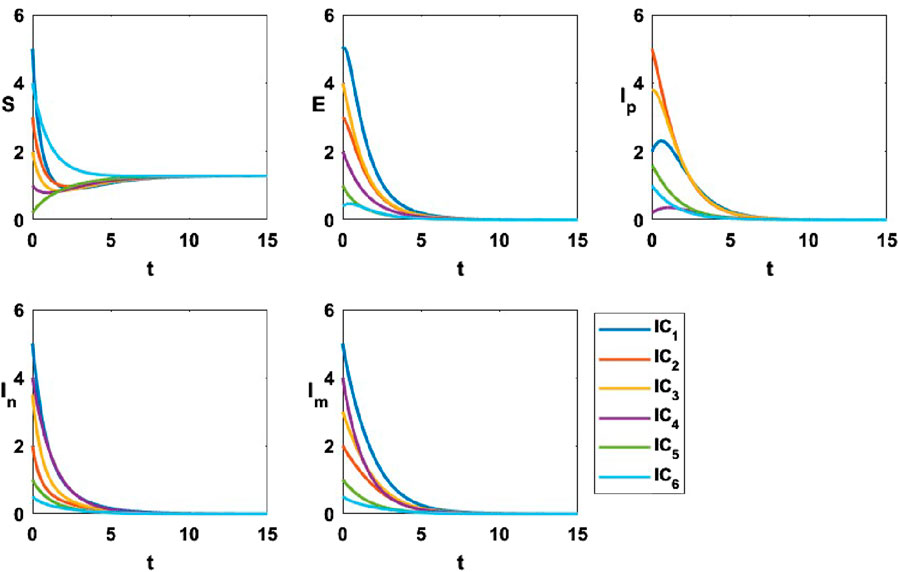
Figure 2. The variational curves of $S$, $E$, $I_p$, $I_n$ and $I_m$ provide insight into the global stability of the dissemination-free equilibrium for ${\mathbf{R}}_{\mathbf{0}}=0.0964286<1$.

3.3 Endemic equilibrium

The endemic equilibrium represents a steady-state solution where dissemination persists in the system at a constant level. Analyzing the stability of this equilibrium provides insight into the long-term behavior of the system, helping to identify conditions under which dissemination persists or diminishes over time.

Theorem 4. For the model defined by (1), the endemic equilibrium, $P_2$, is locally asymptotically stable when the basic reproduction number ${\mathbf{R}}_{\mathbf{0}}>1$.

Proof. We define the following coefficients

$\begin{array}{cc}\hfill B_0& ={\delta }_1+{\delta }_2+{\mu }_3\hfill \\ \hfill B_1& =\frac{\left({\delta }_1+{\delta }_2+{\mu }_3\right)\left(A\lambda \left({\alpha }_1+{\alpha }_2+{\alpha }_3\right)+{\mu }_3\left({\alpha }_1+{\alpha }_2+{\alpha }_3+{\mu }_2\right)\left({\alpha }_1+{\alpha }_2+{\alpha }_3+{\mu }_2+{\mu }_3\right)\right)}{\left({\alpha }_1+{\alpha }_2+{\alpha }_3+{\mu }_2\right){\mu }_3},\hfill \\ \hfill B_2& =\frac{A\lambda \left({\alpha }_1+{\alpha }_2+{\alpha }_3\right)\left({\delta }_1+{\delta }_2+{\mu }_3\right)\left({\alpha }_1+{\alpha }_2+{\alpha }_3+{\mu }_2+{\mu }_3\right)}{\left({\alpha }_1+{\alpha }_2+{\alpha }_3+{\mu }_2\right){\mu }_3},\hfill \\ \hfill B_3& =\left({\delta }_1+{\delta }_2+{\mu }_3\right)\left(A\lambda \left({\alpha }_1+{\alpha }_2+{\alpha }_3\right)-{\mu }_1\left({\alpha }_1+{\alpha }_2+{\alpha }_3+{\mu }_2\right){\mu }_3\right).\hfill \end{array}$

Then, the characteristic polynomial of the Jacobian matrix (Equation 10) corresponding to $P_2$ is

$\left(\xi +{\delta }_1+{\delta }_2+{\mu }_3\right)\left(\xi +2\omega \sqrt{k^2+4l}\right)\left(B_0{\xi }^3+B_1{\xi }^2+B_2\xi +B_3\right)=0.$

It is evident that $B_0$, $B_1$ and $B_2$ are all positive. Furthermore, the condition in (11) for the existence of the endemic equilibrium, guarantees that $B_3$ and $B_1{B}_2-B_0{B}_3$ remain also positive. Consequently, using the Routh-Hurwitz criterion, we determine that $P_2$, when it exists, is locally asymptotically stable.

The inequality in (Equation 6) can be reformulated in terms of ${\mathbf{R}}_{\mathbf{0}}$ defined in (Equation 9), yielding the relation

$\left({\alpha }_1+{\alpha }_2+{\alpha }_3\right)\left({\mathbf{R}}_{\mathbf{0}}-1\right)>0.$

This reformulation highlights that the endemic equilibrium is asymptotically stable for ${\mathbf{R}}_{\mathbf{0}}>1$.

Figure 3 illustrates the surface corresponding to ${\mathbf{R}}_{\mathbf{0}}=1$ for a fixed ${\mu }_2=0.8$, with the $x$-axis representing ${\alpha }_1+{\alpha }_2+{\alpha }_3$, the $y$-axis representing $\lambda /{\mu }_3$, and the $z$-axis representing ${\mu }_1/A$. Parameter values below this surface indicate that the dissemination-free equilibrium is asymptotically stable, whereas values above the surface signify the asymptotic stability of the endemic equilibrium.

Figure 3

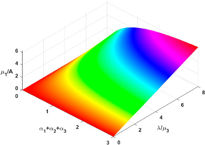
Figure 3. Surface corresponding to ${\mathbf{R}}_{\mathbf{0}}=1$ for a fixed ${\mu }_2=0.8$.

Theorem 5. The endemic equilibrium, $P_2$, of the model defined by (1) is globally asymptotically stable within $\mathrm{\Omega }$ whenever ${\mathbf{R}}_{\mathbf{0}}>1$.

Proof. We consider a nonlinear Lyapunov function of the Goh–Volterra type, structured as

$V\left(x\right)={\displaystyle \sum _{i=1}^n}{c}_i\left(x_i-x_i^{*}-x_i^{*}\ln \frac{x_i}{x_i^{*}}\right),$

which is particularly well-suited for systems with nonlinear interactions, such as those observed in biological or ecological models. Here, $x_i*$ represents the equilibrium value of the $i$-th state variable, and $c_i>0$ are positive constants. These functions are non-negative, achieving their minimum value at the equilibrium $x_i*$.

Let us define the following Lyapunov function of this type for the model given by (1)

$V\left(P\right)=\left(S-S^{*}-S^{*}\ln \frac{S}{S^{*}}\right)+\left(E-E^{*}-E^{*}\ln \frac{E}{E^{*}}\right)+C\left(I-I^{*}-I^{*}\ln \frac{I}{I^{*}}\right),(12)$

where $P=(S,E,I)$, $I=I_p+I_n+I_m$, and $C$ is a positive parameter that will later be determined to satisfy the necessary conditions, particularly those related to the derivative of the Lyapunov function.

By differentiating (Equation 12) and substituting the expressions for the derivatives defined in (1), we obtain

$\begin{array}{cc}\hfill V^{\prime }\left(P\right)& =S^{\prime }-S^{*}\frac{S^{\prime }}{S}+E^{\prime }-E^{*}\frac{E^{\prime }}{E}+C\left(I^{\prime }-I^{*}\frac{I^{\prime }}{I}\right)\hfill \\ \hfill & =\left(1-\frac{S^{*}}{S}\right)\left(A-\lambda SI-{\mu }_{1}S\right)+\left(1-\frac{E^{*}}{E}\right)\left(\lambda SI-\left(\alpha +{\mu }_2\right)E\right)\hfill \\ \hfill & +C\left(1-\frac{I^{*}}{I}\right)\left(\alpha E-{\mu }_{3}I\right)\hfill \end{array}(13)$

where $\alpha ={\alpha }_1+{\alpha }_2+{\alpha }_3$. At $P_2$, solving for $A$ from the first equation of system (1) yields $A=\lambda S*I*+{\mu }_{1}S*$. Substituting this into (Equation 13) and simplifying, we can group the remaining terms as follows

$\begin{array}{ll}\hfill V^{\prime }\left(P\right)& =\lambda S^{*}{I}^{*}+2{\mu }_1{S}^{*}-{\mu }_{1}S-\left(\lambda I^{*}+{\mu }_1\right)\frac{{\left(S^{*}\right)}^2}{S}-\lambda SI\frac{E^{*}}{E}\hfill \\ \hfill & +\left(\alpha +{\mu }_2\right)E^{*}-C\left(\alpha \frac{E}{I}-{\mu }_3\right)I^{*}+W\left(P\right)\hfill \end{array}$

where $W(P)=\lambda S*I-(\alpha +{\mu }_2)E+C\alpha E-C{\mu }_{3}I$.

We set $W(P)=0$; that is,

$\lambda S^{*}I-\left(\alpha +{\mu }_2\right)E+C\alpha E-C{\mu }_{3}I=0.(14)$

A small deviation from the steady state, derived from (Equations 1 and 14), leads to $C=\frac{\lambda }{{\mu }_3}S*$, $\alpha +{\mu }_2=\lambda \frac{S*I*}{E*}$ and $\alpha ={\mu }_3\frac{I^{*}}{E^{*}}$. Substituting these values in (Equation 3), we express the derivative of the Lyapunov function as

$V^{\prime }\left(P\right)=\lambda S^{*}{I}^{*}\left(3-\frac{S^{*}}{S}-\frac{I^{*}}{I}\frac{E}{E^{*}}-\frac{S}{S^{*}}\frac{I}{I^{*}}\frac{E^{*}}{E}\right)+{\mu }_1{S}^{*}\left(2-\frac{S^{*}}{S}-\frac{S}{S^{*}}\right).$

Since the arithmetic mean is greater than or equal to the geometric mean, we get

$3-\frac{S^{*}}{S}-\frac{I^{*}}{I}\frac{E}{E^{*}}-\frac{S}{S^{*}}\frac{I}{I^{*}}\frac{E^{*}}{E}\le 0,2-\frac{S^{*}}{S}-\frac{S}{S^{*}}\le 0,$

which implies that $V^{\prime }(P)\le 0$ for ${\mathbf{R}}_{\mathbf{0}}>1$. By LaSalle’s Invariance Principle, it follows that every solution of the system in (1) approaches the unique associated endemic equilibrium as $t\to \infty$, provided ${\mathbf{R}}_{\mathbf{0}}>1$.

Figure 4 presents the system dynamics, utilizing the parameter values $A=4$, $\lambda =0.1$, ${\mu }_1=0.6$, ${\mu }_2=0.2$, ${\mu }_3=0.25$, ${\alpha }_1=0.1$, ${\alpha }_2=0.3$, ${\alpha }_3=0.2$, $\omega =0.05$, ${\delta }_1=0.03$ and ${\delta }_2=0.04$. The system is examined under the same six initial conditions as in Figure 3. With these parameters, the basic reproduction number satisfies ${\mathbf{R}}_{\mathbf{0}}=2>1$, leading to an endemic equilibrium at (3.33,2.5,2.6652,2.7722,1.5625). According to Theorem 5, this equilibrium is globally asymptotically stable. The figure illustrates that, irrespective of the chosen initial conditions, all state variables ultimately settle at the endemic equilibrium.

Figure 4

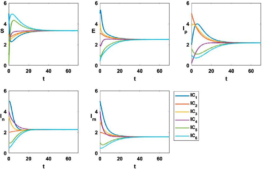
Figure 4. The variational curves of $S$, $E$, $I_p$, $I_n$ and $I_m$ provide insight into the global stability of the endemic equilibrium for ${\mathbf{R}}_{\mathbf{0}}=2>1$.

3.4 Transcritical bifurcation

At ${\mathbf{R}}_{\mathbf{0}}=1$, the system in (1) undergoes a transcritical bifurcation, a phenomenon characterized by an equilibrium whose eigenvalue exhibits a real part that crosses zero. This transition marks a fundamental change in system stability. Using the parameter values $A$, ${\alpha }_1$, ${\alpha }_2$, ${\alpha }_3$, ${\mu }_2$ and ${\mu }_3$ as defined in Figures 4, 5 visualizes the system’s behavior in the $(R_0,I_p+I_n+I_m)$ plane.

Figure 5

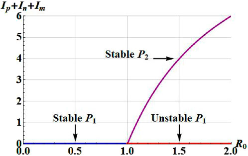
Figure 5. Transcritical bifurcation in the $(R_0,I_p+I_n+I_m)$ plane. The blue curve represents the stable dissemination-free equilibrium, the red curve denotes the unstable equilibrium, and the purple curve corresponds to the stable endemic equilibrium.

The graphical representation highlights the following distinct equilibrium branches in the system.

$•$ The blue curve represents the stable branch of the dissemination-free equilibrium $(P_1)$, where the system remains free from opinion dissemination.

$•$ The red curve denotes the unstable branch of the dissemination equilibrium $(P_1)$, indicating a transition point where stability is lost.

$•$ The purple curve corresponds to the stable endemic equilibrium $(P_2)$, where opinion dissemination persists in a stable state.

3.5 Simulations

3.5.1 Sensitivity analysis of the basic reproduction number

Understanding the sensitivity of the basic reproduction number $({\mathbf{R}}_{\mathbf{0}})$ is crucial for identifying the most influential factors in the opinion spread process. To quantify the impact of each parameter on ${\mathbf{R}}_{\mathbf{0}}$, we compute the normalized sensitivity index defined by

$Y_x^{R_0}=\frac{\partial R_0}{\partial x}\frac{x}{R_0},$

where $Y_x^{{\mathbf{R}}_{\mathbf{0}}}$ measures the relative change in ${\mathbf{R}}_{\mathbf{0}}$ due to a small proportional change in $x$. A positive $Y_x^{{\mathbf{R}}_{\mathbf{0}}}$ indicates that increasing $x$ increases ${\mathbf{R}}_{\mathbf{0}}$, while a negative $Y_x^{{\mathbf{R}}_{\mathbf{0}}}$ means increasing $x$ reduces ${\mathbf{R}}_{\mathbf{0}}$.

Figure 6 presents a bar chart of the sensitivity indices, visually comparing the relative influence of each parameter on ${\mathbf{R}}_{\mathbf{0}}$. The results indicate that $A$ (engagement level) and $\lambda$ (influence rate) have the most significant positive impact on ${\mathbf{R}}_{\mathbf{0}}$, suggesting that increasing engagement or strengthening influence accelerates opinion spread. Conversely, ${\mu }_1$ and ${\mu }_3$ (removal-disengagement rates) strongly decrease ${\mathbf{R}}_{\mathbf{0}}$, indicating that higher disengagement rates help mitigate opinion persistence and reduce polarization effects.

Figure 6

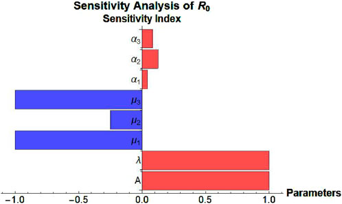
Figure 6. Sensitivity analysis of ${\mathbf{R}}_{\mathbf{0}}$.

The contour plots in Figure 7 illustrate how ${\mathbf{R}}_{\mathbf{0}}$ varies with different system parameters, offering key insights into opinion dissemination which quantifies the balance between influx, transmission, and disengagement rates of susceptibles and communicators, plays a crucial role in shaping ${\mathbf{R}}_{\mathbf{0}}$. As $K=\frac{A\lambda }{{\mu }_1{\mu }_3}$ increases, ${\mathbf{R}}_{\mathbf{0}}$ rises, indicating that a higher influx and transmission relative to disengagement of susceptible and exposed departments leads to sustained opinion spread. Additionally, $\alpha ={\alpha }_1+{\alpha }_2+{\alpha }_3$, representing the total rate at which exposed individuals transition into communicator states (positive, negative, or mixed-emotion), influences the dissemination dynamics but does not guarantee high ${\mathbf{R}}_{\mathbf{0}}$ unless coupled with sufficiently large $K$. Subplot (b) explores the effect of ${\mu }_2$, the disengagement rate of exposed individuals, on ${\mathbf{R}}_{\mathbf{0}}$. The results show that increasing ${\mu }_2$ leads to a decline in ${\mathbf{R}}_{\mathbf{0}}$, highlighting that a higher dropout rate among exposed individuals limits long-term dissemination. The steep color gradients in both subplots suggest a threshold-like transition, where small parameter variations can significantly alter ${\mathbf{R}}_{\mathbf{0}}$.

Figure 7

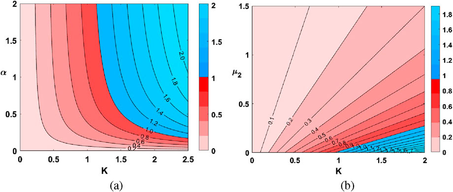
Figure 7. Contour plots of ${\mathbf{R}}_{\mathbf{0}}$ as a function of $K$ and $\alpha$ (a) and $K$ and ${\mu }_2$ (b) where $K=\frac{A\lambda }{{\mu }_1{\mu }_3}$ and $\alpha ={\alpha }_1+{\alpha }_2+{\alpha }_3$. The labels on the contour lines represent the corresponding $R_0$ level values.

3.5.2 Role of engagement in driving polarization and depolarization

Although the model formulation permits time-bounded influxes, the following simulations assume a constant $u(t)=A$ to investigate the system’s long-term behavior and equilibrium dynamics. In this section, we examine how the engagement level, $A$, influences the evolution of public opinion, driving transitions between different opinion states. Here, the parameter $A$ represents the constant influx of new susceptible individuals into the system, determining the rate at which fresh participants enter public discourse. Since $A$ is externally adjustable, it serves as a powerful control mechanism, enabling modifications to the system’s equilibrium and shifting the balance between polarization and depolarization. This implies that in an evolving opinion landscape, adjusting $A$ allows us to steer public discourse, making it a key determinant in shaping long-term ideological stability.

The simulation results, presented in Figure 8, illustrate the influence of 12 different values of $A$, ranging from 0.5 to 6, on the system’s temporal evolution. Each simulation was performed using the initial condition (3,2,4,1,5), ensuring consistency across all cases. A dashed line marks the trajectory for $A=2$, serving as a reference to highlight deviations in system behavior as engagement levels vary.

Figure 8

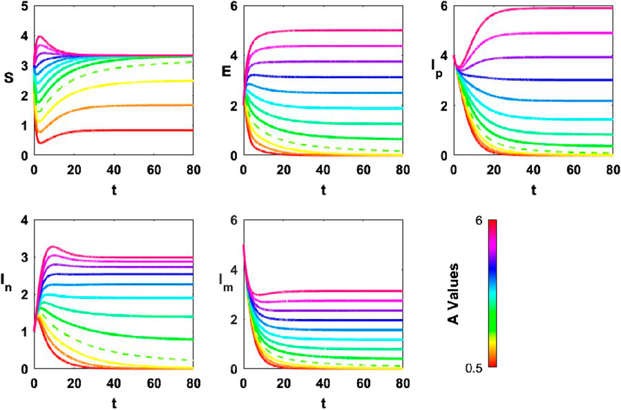
Figure 8. Temporal evolution of opinion groups ($S$, $E$, $I_p$, $I_n$, $I_m$) for different values of engagement level $(A)$. Higher $A$ reinforces polarization by increasing both communicator groups $(I_p,I_n)$, while lower $A$ promotes depolarization as these groups weaken.

For smaller values of $A$, where the inflow to $S$ is relatively low, $I_p$ declines in the early stages before stabilizing. This suggests that when engagement is weak, the ability of $I_p$ to maintain influence diminishes, likely due to insufficient replenishment from the susceptible pool. Meanwhile, $I_n$ exhibits a brief increase before gradually declining to its steady-state, likely due to initial reinforcement within existing networks. However, without sustained engagement, its influence diminishes over time, leading to depolarization as both communicator groups weaken.

As $A$ increases, the dynamics of communicator groups change significantly. Competition initially weakens $I_p$ before it recovers and stabilizes at a higher steady-state. Meanwhile, $I_n$ temporarily benefits from increased exposure before stabilizing at a reduced level. These interactions reflect how, by model construction, engagement supports the persistence of both opposing viewpoints rather than amplifying only one.

For higher values of $A$, the contrast between the two opinionated groups becomes even more pronounced, reinforcing polarization. As engagement increases, both $I_p$ and $I_n$ persist at relatively higher levels, meaning that a larger fraction of the population remains divided into strongly opinionated groups. As expected from the model’s symmetrical structure, increasing engagement sustains both opinionated groups, which aligns with a polarized steady state rather than consensus.

At lower engagement levels, depolarization occurs as both communicator groups gradually lose influence, leading to a more homogeneous opinion landscape. As $I_p$ and $I_n$ decrease over time, opinionated individuals struggle to maintain their influence, resulting in reduced polarization. More individuals either disengage from the discourse or transition into less extreme states, allowing for a more uniform opinion distribution. In the model, lower engagement levels reduce the replenishment of opinionated groups, which leads to a more homogeneous final configuration.

Overall, the simulation results suggest that engagement plays a crucial role in shaping the balance between polarization and depolarization. When engagement is high, ideological divisions are reinforced, with both positive and negative opinion groups persisting at substantial levels. In contrast, when engagement is weak, opinion groups lose their influence over time, leading to a more depolarized system where ideological fragmentation is reduced. These observations, based on the chosen parameter values, highlight the potential of engagement as a mechanism that can either sustain ideological divisions or facilitate depolarization, depending on its intensity.

3.5.3 Role of influence rate in driving polarization and depolarization

In this analysis, the engagement level is fixed at $A=4$, while the influence rate $\lambda$ is varied from 0.01 to 0.95 to examine its role in shaping polarization and depolarization dynamics. In Figure 9, a dashed line at $\lambda =0.09$ is included as a reference, and all other parameters remain consistent with those in Section 3.4.2.

Figure 9

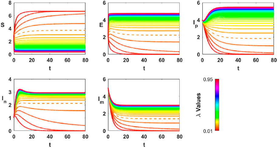
Figure 9. Temporal evolution of opinion groups ($S$, $E$, $I_p$, $I_n$, $I_m$) for different values of influence rate $(\lambda )$. Higher $\lambda$ reinforces polarization by increasing the persistence of communicator groups $(I_p,I_n)$, while lower $\lambda$ weakens their influence, promoting depolarization.

The results suggest that $\lambda$, which controls the strength of influence communicators exert on susceptibles, plays a crucial role in determining whether the system trends toward polarization or depolarization. For smaller values of $\lambda$, both communicator groups weaken over time, indicating that weak influence prevents the long-term persistence of strongly opinionated individuals, facilitating depolarization. Conversely, as $\lambda$ increases, $I_p$ initially decreases but later grows before stabilizing at a higher level, suggesting that stronger influence reinforces opinionated groups rather than weakening them. Meanwhile, $I_n$ initially rises across all $\lambda$ values before declining, with higher $\lambda$ values leading to a more pronounced and sustained increase.

In accordance with the model’s dynamics, stronger influence increases opinion propagation without ensuring convergence to a single viewpoint.

3.5.4 Role of disengagement rate in driving polarization and depolarization

In this analysis, the disengagement level of susceptibles, ${\mu }_1$, is varied from 0.01 to 0.91 to examine its role in shaping polarization and depolarization dynamics. In Figure 10, a dashed line at ${\mu }_1=0.25$ is included as a reference, and all other parameters remain consistent with those in Section 3.4.2. The results indicate that ${\mu }_1$, which controls the rate at which susceptibles leave the system before forming an opinion, significantly influences the persistence of opinionated groups and, consequently, the degree of polarization in the system.

Figure 10

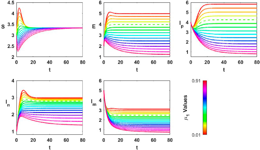
Figure 10. Temporal evolution of opinion groups ($S$, $E$, $I_p$, $I_n$, $I_m$) for different values of disengagement rate $({\mu }_1)$. Higher ${\mu }_1$ leads to depolarization by accelerating the disengagement of susceptibles, reducing the formation of strong opinionated groups. In contrast, a lower ${\mu }_1$sustains polarization by allowing more susceptibles to transition into opinionated states.

For higher values of ${\mu }_1$, the positive communicator population $(I_p)$ decreases over time until it stabilizes at a lower steady-state. This suggests that when susceptibles disengage quickly, fewer individuals transition into the positive communicator group, leading to a weaker influence of strongly opinionated individuals. Meanwhile, the negative communicator group $(I_n)$ initially experiences an increase before declining to a lower steady-state, indicating that a temporary gain in negative opinions is not sustainable under high disengagement rates. In contrast, for lower values of ${\mu }_1$, the behavior of both communicator groups changes significantly. The number of positive communicators decreases at first but later increases before stabilizing at a higher steady-state value, suggesting that when susceptibles remain in the system for longer, more individuals transition into strongly opinionated groups. Similarly, $I_n$ also exhibits an initial rise, but for small ${\mu }_1$, the final steady-state value is significantly higher, indicating that stronger influence sustains both opposing opinion groups for an extended period.

Given the role of ${\mu }_1$ in controlling the outflow from susceptibles, it plays a structural role in determining how opinionated groups evolve in the model. When ${\mu }_1$ is high, both $I_p$ and $I_n$ stabilize at lower levels, suggesting that as susceptibles disengage more rapidly, fewer individuals transition into strong opinion states, leading to depolarization. Conversely, when ${\mu }_1$ is low, both groups persist at higher levels, reinforcing polarization as more individuals remain engaged and committed to their views. These findings confirm that the disengagement rate of susceptibles plays a fundamental role in shaping long-term opinion dynamics, with high disengagement facilitating depolarization and low disengagement reinforcing ideological divisions.

4 Conclusion

In this study, we developed and analyzed a compartmental model that captures the nonlinear dynamics of public opinion dissemination under finite-duration interventions. The model incorporates five interacting compartments, including a novel mixed-emotion group, and is driven by a time-dependent influx function representing external engagement. Through rigorous analytical methods, we established the positivity and boundedness of solutions, identified both dissemination-free and endemic equilibrium points, and determined their stability based on the basic reproduction number ${\mathbf{R}}_{\mathbf{0}}$. Furthermore, the system exhibits a transcritical bifurcation at the critical threshold ${\mathbf{R}}_{\mathbf{0}}=1$, illustrating how qualitative changes in system dynamics emerge with varying control parameters.

Our findings suggest that public discourse can indeed be influenced through targeted interventions, particularly via parameters that correspond to policy-relevant levers. In our model, the engagement amplitude $A$, which represents the sudden influx of users into the discourse, is directly modulated by access policies such as temporary bans or re-openings of digital platforms. The timing and duration of such interventions $(t_{\text{int}},T_{\text{int}})$ are similarly under administrative control. Disengagement rates $({\mu }_1,{\mu }_3)$ may be indirectly shaped through algorithmic throttling, content saturation, or platform design that induces fatigue. An important insight from our analysis is the role of the mixed-emotion group in shaping the persistence and direction of polarization. Although its population may remain moderate, the $I_m$ compartment mediates the flow between opposing viewpoints via transition rates ${\delta }_1$ and ${\delta }_2$. Through the bidirectional transitions governed by ${\delta }_1$ and ${\delta }_2$, the $I_m$ compartment mediates exchanges between opposing communicator groups. In our simulations, this mediating role can prolong the coexistence of $I_p$ and $I_n$ and delay convergence to a single dominant group, thereby supporting the persistence of multiple viewpoints. While these flows are linear and do not constitute a regulatory feedback loop in the strict dynamical systems sense, their structural effect is to provide continuous exchange channels that can sustain ideological diversity under certain parameter regimes. Ignoring this group would risk oversimplifying the dynamics of public discourse, especially in digital environments where users increasingly express ambivalent or multifaceted opinions Additionally, the influence strength $\lambda$, though harder to manipulate directly, can be affected by state-run media amplification or suppression strategies.

A key simplification in our model is the use of constant transition rates from exposed individuals to the opinionated compartments. This implies that opinion adoption is governed by internal dispositions rather than social influence at that stage. While this allows for analytical tractability, it overlooks potential feedback effects where individuals might be more likely to adopt the most visible or dominant opinion. Future extensions could relax this assumption by introducing state-dependent transition rates, possibly influenced by the current distribution of $I_p$, $I_n$, $I_m$, to better capture social reinforcement or conformity effects.

Taken together, both our simulations and sensitivity analysis show that tuning these parameters can shift the system between polarized and depolarized states, offering a theoretical foundation for understanding how public discourse might be steered through real-world regulatory actions.

Future work may extend the model to incorporate time-dependent transition rates and influx functions, allowing for the study of non-autonomous regimes and temporally structured interventions. In particular, while our formulation admits a general time-bounded influx $u(t)$, the present analysis is restricted to the constant-influx case in order to facilitate tractable equilibrium and stability results. Addressing the full transient dynamics under variable $u(t)$ would require alternative mathematical tools suited to non-autonomous systems. Furthermore, coupling the system with delayed or feedback-controlled mechanisms could yield richer bifurcation structures and dynamic responses, offering deeper insights into how temporary engagement surges and algorithmic interventions influence the evolution of polarization over time.

Data availability statement

The original contributions presented in the study are included in the article/supplementary material, further inquiries can be directed to the corresponding author.

Author contributions

AD: Writing – original draft, Formal Analysis, Visualization, Methodology, Software, Writing – review and editing, Validation. AP-D: Software, Writing – review and editing, Methodology, Writing – original draft, Conceptualization, Investigation, Visualization, Validation, Formal Analysis. SH: Writing – original draft, Formal Analysis, Methodology, Validation, Investigation, Writing – review and editing.

Funding

The author(s) declare that no financial support was received for the research and/or publication of this article.

Conflict of interest

The authors declare that the research was conducted in the absence of any commercial or financial relationships that could be construed as a potential conflict of interest.

Generative AI statement

The author(s) declare that no Generative AI was used in the creation of this manuscript.

Any alternative text (alt text) provided alongside figures in this article has been generated by Frontiers with the support of artificial intelligence and reasonable efforts have been made to ensure accuracy, including review by the authors wherever possible. If you identify any issues, please contact us.

Publisher’s note

All claims expressed in this article are solely those of the authors and do not necessarily represent those of their affiliated organizations, or those of the publisher, the editors and the reviewers. Any product that may be evaluated in this article, or claim that may be made by its manufacturer, is not guaranteed or endorsed by the publisher.

References

1. Ataş F, Demirci A, Özemir C. Bifurcation analysis of friedkin–johnsen and hegselmann–krause models with a nonlinear interaction potential. Mathematics Comput Simulation (2021) 185:676–86. doi:10.1016/j.matcom.2021.01.012

CrossRef Full Text | Google Scholar

2. Baumann F, Lorenz-Spreen P, Sokolov IM, Starnini M. Modeling echo chambers and polarization dynamics in social networks. Phys Rev Lett (2020) 124:048301. doi:10.1103/physrevlett.124.048301

PubMed Abstract | CrossRef Full Text | Google Scholar

3. Castellano C, Fortunato S, Loreto V. Statistical physics of social dynamics. Rev Mod Phys (2009) 81:591–646. doi:10.1103/RevModPhys.81.591

CrossRef Full Text | Google Scholar

4. Chen X, Liu Q, Zhang M, Yang Z. Dynamical interplay between the dissemination of scientific knowledge and rumor spreading in emergency. Physica A: Stat Mech its Appl (2019) 526:120808. doi:10.1016/j.physa.2019.120808

CrossRef Full Text | Google Scholar

5. Daley D, Kendall D. Epidemics and rumours. Nature (1965) 204:1118. doi:10.1038/2041118a0

PubMed Abstract | CrossRef Full Text | Google Scholar

6. Deffuant G, Neau D, Amblard F, Weisbuch G. Mixing beliefs among interacting agents. Adv Complex Syst (2000) 3:87–98. doi:10.1142/S0219525900000078

CrossRef Full Text | Google Scholar

7. Diekmann O, Heesterbeek JAP, Roberts MG. The construction of next-generation matrices for compartmental epidemic models. J R Soc Interf (2010) 7:873–85. doi:10.1098/rsif.2009.0386

PubMed Abstract | CrossRef Full Text | Google Scholar

8. Dong S, Wang H, Zhao Y, Wei J, Zhang X. Multilingual seir public opinion propagation model with social enhancement mechanism and cross transmission mechanisms. Scientific Rep (2024) 14:82024. doi:10.1038/s41598-024-82024-3

CrossRef Full Text | Google Scholar

9. Fang M, Li L-N, Yang L. Social network public opinion research based on s-seir epidemic model. In: 2019 IEEE international conference on cloud computing technology and science (CloudCom). IEEE (2019). p. 374–9. doi:10.1109/CloudCom.2019.00069

CrossRef Full Text | Google Scholar

10. Galston WA. Political knowledge, political engagement, and civic education. Annu Rev Polit Sci (2001) 4:217–34. doi:10.1146/annurev.polisci.4.1.217

CrossRef Full Text | Google Scholar

11. Geng L, He Y, Tang L, Chen W, Wang K. Online public opinion dissemination model and simulation under media intervention from different perspectives. Chaos, Solitons and Fractals (2023) 166:112959. doi:10.1016/j.chaos.2022.112959

CrossRef Full Text | Google Scholar

12. Goffman W, Newill V. Generalization of epidemic theory: an application to the transmission of ideas. Nature (1964) 204:225–8. doi:10.1038/204225a0

PubMed Abstract | CrossRef Full Text | Google Scholar

13. Hegselmann R, Krause U. Opinion dynamics and bounded confidence: models, analysis and simulation. J Artif Societies Social Simulation (2002) 5. doi:10.18564/jasss.372

CrossRef Full Text | Google Scholar

14. Ishii A, Okano N, Nishikawa M. Social simulation of intergroup conflicts using a new model of opinion dynamics. Front Phys (2021) 9:640925. doi:10.3389/fphy.2021.640925

CrossRef Full Text | Google Scholar

15. Laguna MF, Risau Gusman S, Abramson G, Gonçalves S, Iglesias JR. The dynamics of opinion in hierarchical organizations. Physica A: Stat Mech its Appl (2005) 351:580–92. doi:10.1016/j.physa.2004.11.064

CrossRef Full Text | Google Scholar

16. Lee J-SF, Tatiana LZ, Arika HM, Behrooz S, Forrest L, Iris V, et al. (2015). The complexities of agent-based modeling output analysis. J Artif Soc S 18. 4. doi:10.18564/jasss.2897

CrossRef Full Text | Google Scholar

17. Lee W, Yang S-G, Kim BJ. The effect of media on opinion formation. Physica A: Stat Mech its Appl (2022) 595:127075. doi:10.1016/j.physa.2022.127075

CrossRef Full Text | Google Scholar

18. Li J, Liu Y, Wang X, Zhao Q. Mechanism study of social media overload on health self-efficacy and anxiety. Heliyon (2024) 10:e1277846. doi:10.1016/j.heliyon.2024.e1277846

CrossRef Full Text | Google Scholar

19. Li L, Li Y, Zhang J. Fractional-order sir model for predicting public opinion dissemination in social networks. Eng Lett (2023) 31.

Google Scholar

20. Lorenz J. Continuous opinion dynamics under bounded confidence: a survey. Int J Mod Phys C (2007) 18:1819–38. doi:10.1142/S0129183107011789

CrossRef Full Text | Google Scholar

21. Lorenz J. Repeated averaging and bounded confidence modeling, analysis and simulation of continuous opinion dynamics. Universität Bremen (2007). Ph.D. thesis.

Google Scholar

22. Lv Y, Wang Z, Zhang H, Zhang X. Research on panic spread and decision behavior in a delayed seir evolutionary game model under an emergency. Scientific Rep (2023) 13: 44116. doi:10.1038/s41598-023-44116-4

CrossRef Full Text | Google Scholar

23. Macal CM, North MJ. “Tutorial on agent-based modeling and simulation,” in Proceedings of the Winter Simulation Conference, 2005. (IEEE). 14. doi:10.1109/WSC.2005.1574234

CrossRef Full Text | Google Scholar

24. Müller B, Balbi S. Standardized and transparent model descriptions for agent-based models: current status and prospects. Environ Model and Softw (2014) 55:156–63. doi:10.1016/j.envsoft.2014.01.029

CrossRef Full Text | Google Scholar

25. Pang X, Zhang Y, Li X, Wang H. How differential dimensions of social media overload influence fatigue: an empirical study during the covid-19 pandemic. Int J Environ Res Public Health (2023) 20:9818937. doi:10.3390/ijerph20031893

CrossRef Full Text | Google Scholar

26. Pranesh S, Gupta S. Exploring cognitive inertia in opinion dynamics using an activity-driven model. Chaos, Solitons and Fractals (2025) 191:115879. doi:10.1016/j.chaos.2024.115879

CrossRef Full Text | Google Scholar

27. Qin X, Wu Z, Chen L, Zhang H. The impact of social media fatigue on disengagement: evidence from digital discourse analysis. Front Psychol (2024) 15:1277846. doi:10.3389/fpsyg.2024.1277846

PubMed Abstract | CrossRef Full Text | Google Scholar

28. Qin Z, Li S, Qi H, Liu S, Meng G, Luo M. Analyze and solve the network public opinion communication based on the improved seir model. 3rd Int Conf Appl Math Model Intell Comput (CAMMIC 2023) (Spie) (2023) 12756:1101–12. doi:10.1117/12.2685942

CrossRef Full Text | Google Scholar

29. Sen P, Chakrabarti BK. Sociophysics: an introduction. Oxford: Oxford University Press (2014).

Google Scholar

30. Smajgl A, Barreteau O. Empirical calibration of agent-based models–challenges and approaches (2014). Springer1. doi:10.1007/978-1-4614-6134-0

CrossRef Full Text | Google Scholar

31. Taylor SE. Decision fatigue and cognitive overload in public engagement. J Cogn Psychol (2021) 33:515–30. doi:10.1080/20445911.2021.1942103

CrossRef Full Text | Google Scholar

32. Wang X, Lin X, Zhong X, Zhang Y, Qiu C. A rumor reversal model of online health information during the covid-19 epidemic. Inf Process and Management (2021) 58:102731. doi:10.1016/j.ipm.2021.102731

PubMed Abstract | CrossRef Full Text | Google Scholar

33. Woo J, Son J, Chen H. An sir model for violent topic diffusion in social media. In: Proceedings of 2011 IEEE international conference on intelligence and security informatics (2011). p. 15–9. doi:10.1109/ISI.2011.5984043

CrossRef Full Text | Google Scholar

34. Xia H, Huili W, Zhaoguo X. Opinion dynamics: a multidisciplinary review and perspective on future research. Int J Knowledge Syst Sci (Ijkss) (2011) 2:72–91. doi:10.4018/jkss.2011100106

CrossRef Full Text | Google Scholar

35. Yan Z, Zhou X, Du R. An enhanced sir dynamic model: the timing and changes in public opinion in the process of information diffusion. Electron Commerce Res (2024) 24:2021–44. doi:10.1007/s10660-022-09608-x

CrossRef Full Text | Google Scholar

36. Yuan J, Shi J, Wang J, Liu W. Modelling network public opinion polarization based on sir model considering dynamic network structure. Alexandria Eng J (2022) 61:4557–71. doi:10.1016/j.aej.2021.10.014

CrossRef Full Text | Google Scholar

37. Zhu H, Lv W, Xu W, Liu P. Effect of users’ opinion evolution on information diffusion in online social networks. Physica A: Stat Mech its Appl (2018) 492:2034–45. doi:10.1016/j.physa.2017.11.106

CrossRef Full Text | Google Scholar