An efficient explicit group method for time fractional Burgers equation

Fractional Burgers-type equations are essential mathematical models for describing the cumulative effect of wall friction through the boundary layer, along with the unidirectional propagation of weakly nonlinear acoustic waves. It is a major challenge to develop efficient, stable, and accurate numerical schemes that simulate the corresponding complex physical phenomena due to the nonlinearity and nonlocality properties in these equations. The objective of this article is to design a linearized modified fractional explicit group method for solving the two-dimensional time-fractional Burgers equation with suitable initial and boundary conditions. For the construction of the proposed method, the $L_1$ discretization formula is used to handle the fractional temporal derivative, whereas a linearized difference scheme on a coarse mesh is employed to approximate the spatial derivatives. Meanwhile, a linearized Crank–Nicolson difference method (LCNDM) is formulated for checking the efficiency of the proposed method. The stability and convergence of the presented methods are rigorously studied and proven. Numerical simulations are performed, and the results are reported in terms of error norm and CPU time, demonstrating that the linearized grouping method reduces computation time by 70%–90% while maintaining comparable accuracy to the linearized Crank–Nicolson method in solving the time-fractional Burgers model.

1 Introduction

In recent years, the interest in the fractional calculus (FC), dealing with differential and integral operators of arbitrary orders, has witnessed a remarkable mutation. In contrast to the classical differential operator, the fractional differential operator considers not only the immediate past of the relevant function but also its historical values. The memory and history dependence properties of fractional differential operators are considered the golden features of FC, which make it favorable for describing numerous real-life complex phenomena. Fractional differential equations are the basic tools of FC for handling the anomalous phenomena in diverse complex systems. For extra information on the definitions and properties of FC, the reader can refer to [1–3]. Fractional differential equations can be divided into fractional ordinary differential equations (FODEs) and fractional partial differential equations (FPDEs). In the past few years, many researchers and scholars from different scientific backgrounds have utilized fractional differential equations (FODEs and FPDEs) as efficient mathematical models for dealing with numerous real-world complex problems. For instance, among recent applications, fractional differential equations have been used for describing several phenomena, including COVID-19 transmission [4], regulation of atmospheric carbon dioxide levels, and battery temperature estimation [5]. Other interesting works highlighting the importance and applications of FC can be found in [6–9].

In line with the wide-ranging applications of FC and to better understand complex real-life systems, solving fractional differential equations has become indispensable. This study is concerned with the solution of an important type of FPDEs, namely, the time-fractional Burgers equation. An overview of the general form and significance of the aforementioned mathematical model is provided in the next section. Due to the unusual properties of fractional differential operators, such as the violation of the chain rule, Leibniz rule, and semigroup property, explicit analytic solutions of FPDEs cannot be easily obtained [10]. As a result, approximate analytical and numerical methods for solving FPDEs have received significant attention. The homotopy analysis method [11], variational iterative method [12, 13], perturbation analysis method [14], and differential transform method [14] are examples of approximate analytical methods that have been applied for solving the fractional Burgers equation. One drawback of the aforementioned analytical methods is that most of them consider only the initial condition and neglect the spatial boundary conditions of the fractional Burgers model. However, boundary conditions are of great importance for characterizing and modeling real-world processes. To surmount this issue, numerical methods capable of solving the fractional Burgers model with suitable initial and boundary conditions can be developed, which is the first motivation of this work.

In the literature, several research articles are devoted to solving the time-fractional Burgers equation numerically. In this study, we recall some of them. [15] introduced an implicit spectral collocation method for solving the one-dimensional time-fractional Burgers equation. The unconditional stability and convergence are proved theoretically and affirmed through numerical experiments. [16] established a second-order linearized difference scheme to solve the one-dimensional time-fractional Burgers equation. The theoretical analysis shows that the scheme is unconditionally stable and convergent. [17] combined the finite integration method with the shifted Chebyshev polynomials to solve the one- and two-dimensional time-fractional Burgers equations. [18] scrutinized an implicit difference scheme for the solution of the one-dimensional time-fractional Burgers equation. [19] utilized the L1 scheme on a temporal graded mesh and the Legendre–Galerkin spectral approach in space to account for the solution of the one-dimensional time-fractional Burgers equation. [20] derived a Crank–Nicolson difference scheme to deal with the one-dimensional time-fractional Burgers equation. The stability and convergence of the proposed scheme are not discussed. A computational scheme based on a finite difference in time and a cubic trigonometric B-spline in space for the one-dimensional time-fractional Burgers equation was suggested by [21]. [22] constructed a non-standard finite difference method for the one-dimensional complex-order Burgers equation. [23] suggested a finite difference scheme for the one-dimensional fractional Burgers equation involving the Atangana–Baleanu temporal derivative. [24] used the finite difference technique in time and the extended cubic B-spline approach in space for the solution of the one-dimensional time-fractional Burgers equation. [25] developed a space–time spectral collocation method to solve the one-dimensional time-fractional Burgers equation. [26] introduced a linear implicit difference scheme for the one-dimensional fractional Burgers equation, including the generalized temporal Atangana–Baleanu derivative. An explicit decoupled group method for the two-dimensional time-fractional Burgers equation was introduced by [27]. [28] designed a finite difference scheme for the one-dimensional time-fractional Burgers model subject to artificial boundary conditions on unbounded domains. [29] proposed a differential quadrature method based on a modified hybrid B-spline basis function for the one-dimensional time-fractional Burgers equation. [30] developed a local projection stabilization virtual element method for the solution of the two-dimensional time-fractional Burgers equation. Other recent numerical treatments of the time-fractional Burgers equation can be found in [31–33]. We note that the mentioned research work is almost limited to one-dimensional problems, while the numerical treatment of two-dimensional Burgers models is limited in the literature. This is our second motivation for finding the numerical solution of the two-dimensional time-fractional Burger model presented in the next section.

The definition of the time-fractional derivative has an integral form, which leads to the non-locality of the fractional differential operator. This means that the storage of the solution values at all previous time levels is crucial for computing the solution at the current time level. Such a phenomenon causes several difficulties and challenges related to the computational complexity and theoretical analysis of time FPDEs. For instance, a two-dimensional time-fractional model with mesh size $N$ in the temporal direction and mesh points $M$ in the spatial direction requires a computational cost of $O(N^2)$ and a storage requirement of $O(NM)$. The implementation process of a long-time or large-domain simulation is still very difficult, even with high-performance computers. Consequently, the development of unconditionally stable, accurate, and computationally efficient numerical schemes for solving multi-dimensional time FPDEs is considered one of the open problems in this field [34]. This is the third motivation for our work.

In the last few years, explicit group methods have gained popularity in the numerical research field. These methods can be established based on finite difference approximations, where the solution is computed iteratively on a group of spatial mesh points rather than on a single point in the point-wise iterative schemes. Fractional diffusion equations [35–38], fractional cable equations [39–41], fractional mobile/immobile equations [42, 43], and fractional telegraph equations [44, 45] are solved successfully using these methods. Explicit group iterative methods can effectively refine the spectral properties of the iteration matrix and accelerate the rate of convergence of numerical algorithms. In addition, they can be implemented on parallel computers, making them a favored choice for simulation purposes. Moreover, since they rely on the finite difference method, explicit group methods inherit simplicity and universal applicability to a wide range of fractional problems. The primary goal of this paper is to propose an explicit group approach, namely, the linearized modified fractional explicit group method (LMFEGM), for the numerical solution of the two-dimensional time-fractional Burgers model. For the construction of the LMFEGM, we deal with the time-fractional derivative using the L1 discretization formula, while a linearized difference scheme based on double mesh spacing is used for the partial space derivatives. To evaluate the computational efficiency of the proposed method for solving the fractional Burgers equation, a linearized Crank–Nicolson difference method (LCNDM) is established as a reference method. The stability and convergence of the presented methods are analyzed in detail using the Fourier method. Furthermore, several numerical experiments are carried out to verify our considerations. The corresponding numerical results show the efficiency of the LMFEGM in terms of accuracy and reduction of computing effort compared to the LCNDM. To our knowledge, the current work, driven by the stated motivations, is novel as no attempt to solve the fractional Burgers equation using the LMFEGM has been reported in the literature.

In summary, the contributions of this work are listed as follows:

$•$ the development of the LMFEGM for efficiently solving the two-dimensional time fractional Burgers equation;

$•$ the derivation of the LCNDM as a reference method for verifying accuracy and computational efficiency;

$•$ the analysis of the stability and convergence properties of the proposed scheme; and

$•$ the execution and discussion of several numerical simulations.

The remainder of this article is arranged as follows. Section 2 provides an overview of the considered time-fractional Burgers model. Section 3 is devoted to the formulation of the proposed linearized numerical schemes. The stability and convergence properties of the presented methods are discussed in complete detail in Sections 4, 5, respectively. In Section 6, we implement several numerical experiments to test the performance and validate the theoretical statements. Finally, a brief conclusion is provided in Section 7.

2 Time-fractional Burgers model

The Burgers equation, named after J. M. Burgers (1895–1981), is one of the basic partial differential equations (PDEs) with numerous applications in science and engineering. In the literature, the solution and analysis of PDEs are one of the major topics in applied mathematics, due to their significant role in describing numerous phenomena in physics, chemistry, finance, biology, viscoelasticity, fluid mechanics, etc. In particular, the Burgers mathematical model has been applied in various disciplines such as gas dynamics, turbulent flows, shock wave theory, longitudinal elastic waves in isotropic solids, nonlinear wave propagation, growth of molecular interfaces, sedimentation of polydispersive suspensions and colloids, cosmology, and traffic flow. Furthermore, Burgers-type equations can be utilized as a reference for solving the Navier–Stokes equations as they share a similar structure but lack a pressure gradient. For details on applications of the Burgers equation, readers can refer to [46]. The general form of the one-dimensional Burgers equation is as follows:

$w_t\left(x,t\right)-\nu w_{xx}\left(x,t\right)+w\left(x,t\right)w_x\left(x,t\right)=f\left(x,t\right).(1)$

The abovementioned integer-order Burgers equation is a mathematical model involving nonlinear propagation effects along with diffusion effects. Due to the fact that integer-order derivatives cannot describe the memory and hereditary properties of complex systems compared to fractional-order derivatives, many researchers have extended Equation 1 to its fractional-order counterpart. This can be achieved by replacing the integer-order derivatives in Equation 1 with time and/or space fractional derivatives to capture the true behavior of physical phenomena. In this work, we consider the following two-dimensional time-fractional Burgers model:

$\left\{\begin{array}{c}{}_0{}^{C}D_t^{\alpha }w(\mathbf{x},t)-\nu \mathrm{\Delta }w(\mathbf{x},t)+w(\mathbf{x},t)(\nabla w(\mathbf{x},t)\cdot \mathbf{1})=f(\mathbf{x},t),(\mathbf{x},t)\in \mathrm{\Omega }\times \left(0\right.,\left.T\right],\hfill \\ w(\mathbf{x},0)=g_0(\mathbf{x}),\mathbf{x}\in \mathrm{\Omega }\cup \partial \mathrm{\Omega },\hfill \\ w(\mathbf{x},t)=g_1(\mathbf{x},t),(\mathbf{x},t)\in \partial \mathrm{\Omega }\times \left(0\right.,\left.T\right],\hfill \end{array}\right.(2)$

where $\mathbf{x}=(x,y)$, $\mathbf{1}=(\mathrm{1,1})$, $\mathrm{\Delta }w(\mathbf{x},t)=w_{xx}(\mathbf{x},t)+w_{yy}(\mathbf{x},t)$ is the Laplacian operator, and $w(\mathbf{x},t)(\nabla w(\mathbf{x},t)\cdot \mathbf{1})=w(\mathbf{x},t)(w_x(\mathbf{x},t)+w_y(\mathbf{x},t))$. In this equation, $\mathrm{\Omega }=[0,L_x]\times [0,L_y]$ is a rectangular bounded domain included in $R^2$, and $\partial \mathrm{\Omega }$ is its boundary. $\nu =1/RE$, where $RE$ is the Reynolds number used to describe the transport properties of a fluid or a particle moving in a fluid [47], and $g_0(\mathbf{x})$, $g_1(\mathbf{x},t)$, and $f(\mathbf{x},t)$ are known smooth functions. ${}_0{}^{C}D_t^{\alpha }$ $w(\mathbf{x},t)$ is the Caputo-type fractional temporal derivative, which is defined as follows:

${}_0{}^{C}D_t^{\alpha }w\left(\mathbf{x},t\right)=\left\{\begin{array}{c}\frac{1}{\mathrm{\Gamma }\left(1-\alpha \right)}{\int }_0^t{\left(t-\xi \right)}^{-\alpha }\frac{\partial w\left(\mathbf{x},\xi \right)}{\partial \xi }d\xi ,0<\alpha <1,\hfill \\ \frac{\partial w\left(\mathbf{x},t\right)}{\partial t},\alpha =1.\hfill \end{array}\right.$

The involvement of the Caputo fractional temporal derivative in the Burgers model (Equation 2) makes it suitable for describing the cumulative effect of wall friction through the boundary layer, along with the unidirectional propagation of weakly nonlinear acoustic waves [19, 48]. Due to the added complexity of handling the fractional derivative and nonlinear convection term, exact analytic solutions of the fractional Burgers equation are not easy to obtain. Consequently, the development of efficient, accurate, and stable numerical schemes for solving such equations is of utmost importance. In the next section, we propose the LCNDM and the LMFEGM for solving the model problem (Equation 2).

3 Formulation of the linearized schemes

3.1 Linearized Crank–Nicolson difference scheme

In order to establish a discrete form of the fractional Burgers model (Equation 2), its appearing integer and fractional derivatives can be replaced with their corresponding finite difference approximations. We introduce some notations to facilitate our formulation. We assume that $\mathrm{\Delta }x=L_x/M_x$, $\mathrm{\Delta }y=L_y/M_y$, and $\mathrm{\Delta }t=T/N$ are some spatial and temporal increments, where $M_x$, $M_y$, and $N$ are the given positive integers. A spatial mesh is defined as $x_i=i\mathrm{\Delta }x$, where $0\le i\le M_x$, and $y_j=j\mathrm{\Delta }y$, where $0\le j\le M_y$, and a temporal mesh is given by $t_n=n\mathrm{\Delta }t$, where $0\le n\le N$.

The grid functions are defined as follows:

$w_{i,j}^n=w\left(x_i,y_j,t_n\right),f_{i,j}^n=f\left(x_i,y_j,t_n\right),0\le i\le M_x,0\le j\le M_y,0\le n\le N.$

We assume that $w=\{w_{i,j}^n|0\le i\le M_x,0\le j\le M_y,0\le n\le N\}$ is a grid function. The following notations are introduced:

$\begin{array}{ll}\hfill {\left.\frac{{\partial }^{2}w}{\partial x^2}\right|}_{i,j}^{n+1/2}& =\frac{1}{2}\left[\frac{w_{i+1,j}^{n+1}-2w_{i,j}^{n+1}+w_{i-1,j}^{n+1}}{{\left(\mathrm{\Delta }x\right)}^2}+\frac{w_{i+1,j}^n-2w_{i,j}^n+w_{i-1,j}^n}{{\left(\mathrm{\Delta }x\right)}^2}\right]\hfill \\ \hfill & +O\left({\left(\mathrm{\Delta }t\right)}^2+{\left(\mathrm{\Delta }x\right)}^2+{\left(\mathrm{\Delta }y\right)}^2\right),\hfill \end{array}(3)$

$\begin{array}{ll}\hfill {\left.\frac{{\partial }^{2}w}{\partial y^2}\right|}_{i,j}^{n+1/2}& =\frac{1}{2}\left[\frac{w_{i,j+1}^{n+1}-2w_{i,j}^{n+1}+w_{i,j-1}^{n+1}}{{\left(\mathrm{\Delta }y\right)}^2}+\frac{w_{i,j+1}^n-2w_{i,j}^n+w_{i,j-1}^n}{{\left(\mathrm{\Delta }y\right)}^2}\right]\hfill \\ \hfill & +O\left({\left(\mathrm{\Delta }t\right)}^2+{\left(\mathrm{\Delta }x\right)}^2\right)+\left.{\left(\mathrm{\Delta }y\right)}^2\right).\hfill \end{array}(4)$

We adopt the technique for linearizing nonlinear convection terms from [49], where the following identities are used:

$\begin{array}{ll}\hfill w^{n+1}{w}_x^{n+1}& =w^{n+1}{w}_x^n+w^n{w}_x^{n+1}-w^n{w}_x^n,\hfill \\ \hfill w^{n+1}{w}_y^{n+1}& =w^{n+1}{w}_y^n+w^n{w}_y^{n+1}-w^n{w}_y^n.\hfill \end{array}$

Accordingly, the nonlinear terms $w{w}_x$ and $w{w}_y$ can be discretized as follows:

${\left.w\frac{\partial w}{\partial x}\right|}_{i,j}^{n+1/2}=\frac{1}{4\mathrm{\Delta }x}\left[w_{i,j}^n\left(w_{i+1,j}^{n+1}-w_{i-1,j}^{n+1}\right)+w_{i,j}^{n+1}\left(w_{i+1,j}^n-w_{i-1,j}^n\right)+O\left({\left(\mathrm{\Delta }t\right)}^2+{\left(\mathrm{\Delta }x\right)}^2\right)\right],(5)$

${\left.w\frac{\partial w}{\partial y}\right|}_{i,j}^{n+1/2}=\frac{1}{4\mathrm{\Delta }y}\left[w_{i,j}^n\left(w_{i,j+1}^{n+1}-w_{i,j-1}^{n+1}\right)+w_{i,j}^{n+1}\left(w_{i,j+1}^n-w_{i,j-1}^n\right)+O\left({\left(\mathrm{\Delta }t\right)}^2+{\left(\mathrm{\Delta }y\right)}^2\right)\right].(6)$

To approximate the fractional temporal derivative in the Caputo sense, we use the $L_1$ discretization scheme [50] as follows:

$\begin{array}{cc}\hfill {\left.\frac{{\partial }^{\alpha }w}{\partial t^{\alpha }}\right|}_{i,j}^{n+1/2}& =\sigma \left[{\eta }_1{w}_{i,j}^n+{\displaystyle \sum _{s=1}^{n-1}}\left({\eta }_{n-s+1}-{\eta }_{n-s}\right)w_{i,j}^s-{\eta }_n{w}_{i,j}^0+\frac{\left(w_{i,j}^{n+1}-w_{i,j}^n\right)}{2^{1-\alpha }}\right]\hfill \\ \hfill & +r_{i,j}^{n+1/2},\hfill \end{array}(7)$

where

$\sigma =\frac{1}{\mathrm{\Gamma }\left(2-\alpha \right){\left(\mathrm{\Delta }t\right)}^{\alpha }},{\eta }_n=\left({\left(n+1/2\right)}^{1-\alpha }-{\left(n-1/2\right)}^{1-\alpha }\right),$

and the truncation error $r_{i,j}^{n+1/2}$ satisfies the following inequality:

$|r_{i,j}^{n+1/2}|\le C{\left(\mathrm{\Delta }t\right)}^{2-\alpha }.$

Given the definition of the Caputo fractional derivative, weak regularity may exist in the exact solution of the time-fractional model (Equation 2) at the initial time. Nevertheless, we assume that the considered problem has a unique and sufficiently smooth exact solution without loss of this constraint.

Substituting Equations 3–7 into Equation 2 yields the following:

$\begin{array}{cc}\hfill & \sigma \left[{\eta }_1{w}_{i,j}^n+{\displaystyle \sum _{s=1}^{n-1}}\left({\eta }_{n-s+1}-{\eta }_{n-s}\right)w_{i,j}^s-{\eta }_n{w}_{i,j}^0+\frac{\left(w_{i,j}^{n+1}-w_{i,j}^n\right)}{2^{1-\alpha }}\right]\hfill \\ \hfill & -\frac{\nu }{2}\left[\frac{w_{i+1,j}^{n+1}-2w_{i,j}^{n+1}+w_{i-1,j}^{n+1}}{{\left(\mathrm{\Delta }x\right)}^2}+\frac{w_{i+1,j}^n-2w_{i,j}^n+w_{i-1,j}^n}{{\left(\mathrm{\Delta }x\right)}^2}\right]\hfill \\ \hfill & -\frac{\nu }{2}\left[\frac{w_{i,j+1}^{n+1}-2w_{i,j}^{n+1}+w_{i,j-1}^{n+1}}{{\left(\mathrm{\Delta }y\right)}^2}+\frac{w_{i,j+1}^n-2w_{i,j}^n+w_{i,j-1}^n}{{\left(\mathrm{\Delta }y\right)}^2}\right]\hfill \\ \hfill & +\frac{1}{4\mathrm{\Delta }x}\left[w_{i,j}^n\left(w_{i+1,j}^{n+1}-w_{i-1,j}^{n+1}\right)+w_{i,j}^{n+1}\left(w_{i+1,j}^n-w_{i-1,j}^n\right)\right]\hfill \\ \hfill & +\frac{1}{4\mathrm{\Delta }y}\left[w_{i,j}^n\left(w_{i,j+1}^{n+1}-w_{i,j-1}^{n+1}\right)+w_{i,j}^{n+1}\left(w_{i,j+1}^n-w_{i,j-1}^n\right)\right]\hfill \\ \hfill & =f_{i,j}^{n+1/2}+O\left({\left(\mathrm{\Delta }t\right)}^{2-\alpha }+{\left(\mathrm{\Delta }x\right)}^2+{\left(\mathrm{\Delta }y\right)}^2\right).\hfill \end{array}(8)$

By dropping higher-order small error terms and replacing $w^n$ with its numerical approximation $W^n$, we obtain the LCNDM:

$\begin{array}{cc}\hfill & \left(1+\frac{\nu m}{{\left(\mathrm{\Delta }x\right)}^2}+\frac{\nu m}{{\left(\mathrm{\Delta }y\right)}^2}+\frac{m}{4\mathrm{\Delta }x}\left(W_{i+1,j}^n-W_{i-1,j}^n\right)+\frac{m}{4\mathrm{\Delta }y}\left(W_{i,j+1}^n-W_{i,j-1}^n\right)\right)W_{i,j}^{n+1}\hfill \\ \hfill & =\left(\frac{\nu m}{2{\left(\mathrm{\Delta }x\right)}^2}-\frac{m}{4\mathrm{\Delta }x}{W}_{i,j}^n\right)W_{i+1,j}^{n+1}+\left(\frac{\nu m}{2{\left(\mathrm{\Delta }x\right)}^2}+\frac{m}{4\mathrm{\Delta }x}{W}_{i,j}^n\right)W_{i-1,j}^{n+1}\hfill \\ \hfill & +\left(\frac{\nu m}{2{\left(\mathrm{\Delta }y\right)}^2}-\frac{m}{4\mathrm{\Delta }y}{W}_{i,j}^n\right)W_{i,j+1}^{n+1}+\left(\frac{\nu m}{2{\left(\mathrm{\Delta }y\right)}^2}+\frac{m}{4\mathrm{\Delta }y}{W}_{i,j}^n\right)W_{i,j-1}^{n+1}\hfill \\ \hfill & +\frac{\nu m}{2{\left(\mathrm{\Delta }x\right)}^2}\left(W_{i+1,j}^n+W_{i-1,j}^n\right)+\frac{\nu m}{2{\left(\mathrm{\Delta }y\right)}^2}\left(W_{i,j+1}^n+W_{i,j-1}^n\right)\hfill \\ \hfill & +\left(1-2^{1-\alpha }{\eta }_1-\frac{\nu m}{{\left(\mathrm{\Delta }x\right)}^2}-\frac{\nu m}{{\left(\mathrm{\Delta }y\right)}^2}\right)W_{i,j}^n+2^{1-\alpha }{\displaystyle \sum _{s=1}^{n-1}}\left({\eta }_{n-s}-{\eta }_{n-s+1}\right)W_{i,j}^s\hfill \\ \hfill & +2^{1-\alpha }{\eta }_n{W}_{i,j}^0+m{f}_{i,j}^{n+1/2},1\le i\le M_x-1,1\le j\le M_y-1,0\le n\le N-1,\hfill \end{array}(9)$

where $m=2^{1-\alpha }\mathrm{\Gamma }(2-\alpha ){(\mathrm{\Delta }t)}^{\alpha }$.

3.2 Linearized grouping scheme

In this section, we introduce the linearized modified fractional explicit group method (LMFEGM) for the Burgers model (Equation 2). The idea of this method is to branch the spatial mesh points at each time level into small, fixed-size groups of points. After that, the numerical solution is computed at each group using an iterative process that involves only a quarter of the entire mesh, which efficiently reduces the computational complexity. For the construction of the LMFEGM, we consider a coarse mesh with spatial spacing $\mathrm{\Delta }x=2h_x$ and $\mathrm{\Delta }y=2h_y$. On this coarse mesh, the finite difference operators (Equations 3–6) can be redefined as follows:

$\begin{array}{ll}\hfill {\left.\frac{{\partial }^{2}w}{\partial x^2}\right|}_{i,j}^{n+1/2}& =\frac{1}{2}\left[\frac{w_{i+2,j}^{n+1}-2w_{i,j}^{n+1}+w_{i-2,j}^{n+1}}{4h_x^2}+\frac{w_{i+2,j}^n-2w_{i,j}^n+w_{i-2,j}^n}{4h_x^2}\right]\hfill \\ \hfill & +O\left({\left(\mathrm{\Delta }t\right)}^2+{\left(\mathrm{\Delta }x\right)}^2+{\left(\mathrm{\Delta }y\right)}^2\right),\hfill \end{array}(10)$

$\begin{array}{ll}\hfill {\left.\frac{{\partial }^{2}w}{\partial y^2}\right|}_{i,j}^{n+1/2}& =\frac{1}{2}\left[\frac{w_{i,j+2}^{n+1}-2w_{i,j}^{n+1}+w_{i,j-2}^{n+1}}{4h_y^2}+\frac{w_{i,j+2}^n-2w_{i,j}^n+w_{i,j-2}^n}{4h_y^2}\right]\hfill \\ \hfill & +O\left({\left(\mathrm{\Delta }t\right)}^2+\left.{\left(\mathrm{\Delta }x\right)}^2\right)+{\left(\mathrm{\Delta }y\right)}^2\right).\hfill \end{array}(11)$

${\left.w\frac{\partial w}{\partial x}\right|}_{i,j}^{n+1/2}=\frac{1}{8h_x}\left[w_{i,j}^n\left(w_{i+2,j}^{n+1}-w_{i-2,j}^{n+1}\right)+w_{i,j}^{n+1}\left(w_{i+2,j}^n-w_{i-2,j}^n\right)+O\left({\left(\mathrm{\Delta }t\right)}^2+{\left(\mathrm{\Delta }x\right)}^2\right)\right],(12)$

${\left.w\frac{\partial w}{\partial y}\right|}_{i,j}^{n+1/2}=\frac{1}{8h_y}\left[w_{i,j}^n\left(w_{i,j+2}^{n+1}-w_{i,j-2}^{n+1}\right)+w_{i,j}^{n+1}\left(w_{i,j+2}^n-w_{i,j-2}^n\right)+O\left({\left(\mathrm{\Delta }t\right)}^2+{\left(\mathrm{\Delta }y\right)}^2\right)\right].(13)$

By combining Equations 10–13 and Equation 7 into Equation 2, we derive the following:

$\begin{array}{cc}\hfill & \sigma \left[{\eta }_1{w}_{i,j}^n+{\displaystyle \sum _{s=1}^{n-1}}\left({\eta }_{n-s+1}-{\eta }_{n-s}\right)w_{i,j}^s-{\eta }_n{w}_{i,j}^0+\frac{\left(w_{i,j}^{n+1}-w_{i,j}^n\right)}{2^{1-\alpha }}\right]\hfill \\ \hfill & -\frac{\nu }{2}\left[\frac{w_{i+2,j}^{n+1}-2w_{i,j}^{n+1}+w_{i-2,j}^{n+1}}{4h_x^2}+\frac{w_{i+2,j}^n-2w_{i,j}^n+w_{i-2,j}^n}{4h_x^2}\right]\hfill \\ \hfill & -\frac{\nu }{2}\left[\frac{w_{i,j+2}^{n+1}-2w_{i,j}^{n+1}+w_{i,j-2}^{n+1}}{4h_y^2}+\frac{w_{i,j+2}^n-2w_{i,j}^n+w_{i,j-2}^n}{4h_y^2}\right]\hfill \\ \hfill & +\frac{1}{8h_x}\left[w_{i,j}^n\left(w_{i+2,j}^{n+1}-w_{i-2,j}^{n+1}\right)+w_{i,j}^{n+1}\left(w_{i+2,j}^n-w_{i-2,j}^n\right)\right]\hfill \\ \hfill & +\frac{1}{8h_y}\left[w_{i,j}^n\left(w_{i,j+2}^{n+1}-w_{i,j-2}^{n+1}\right)+w_{i,j}^{n+1}\left(w_{i,j+2}^n-w_{i,j-2}^n\right)\right]\hfill \\ \hfill & =f_{i,j}^{n+1/2}+O\left({\left(\mathrm{\Delta }t\right)}^{2-\alpha }+{\left(\mathrm{\Delta }x\right)}^2+{\left(\mathrm{\Delta }y\right)}^2\right).\hfill \end{array}$

Neglecting the higher-order small error terms and replacing $w^n$ with its numerical approximation $W^n$ lead to the fully discrete scheme:

$\begin{array}{cc}\hfill & \left(1+\frac{\nu m}{4h_x^2}+\frac{\nu m}{4h_y^2}+\frac{m}{8h_x}\left(W_{i+2,j}^n-W_{i-2,j}^n\right)+\frac{m}{8h_y}\left(W_{i,j+2}^n-W_{i,j-2}^n\right)\right)W_{i,j}^{n+1}\hfill \\ \hfill & =\left(\frac{\nu m}{8h_x^2}-\frac{m}{8h_x}{W}_{i,j}^n\right)W_{i+2,j}^{n+1}+\left(\frac{\nu m}{8h_x^2}+\frac{m}{8h_x}{W}_{i,j}^n\right)W_{i-2,j}^{n+1}\hfill \\ \hfill & +\left(\frac{\nu m}{8h_y^2}-\frac{m}{8h_y}{W}_{i,j}^n\right)W_{i,j+2}^{n+1}+\left(\frac{\nu m}{8h_y^2}+\frac{m}{8h_y}{W}_{i,j}^n\right)W_{i,j-2}^{n+1}\hfill \\ \hfill & +\frac{\nu m}{8h_x^2}\left(W_{i+2,j}^n+W_{i-2,j}^n\right)+\frac{\nu m}{8h_y^2}\left(W_{i,j+2}^n+W_{i,j-2}^n\right)\hfill \\ \hfill & +\left(1-2^{1-\alpha }{\eta }_1-\frac{\nu m}{4h_x^2}-\frac{\nu m}{4h_y^2}\right)W_{i,j}^n+2^{1-\alpha }{\displaystyle \sum _{s=1}^{n-1}}\left({\eta }_{n-s}-{\eta }_{n-s+1}\right)W_{i,j}^s\hfill \\ \hfill & +2^{1-\alpha }{\eta }_n{W}_{i,j}^0+m{f}_{i,j}^{n+1/2},2\le i\le M_x-2,2\le j\le M_y-2,0\le n\le N-1.\hfill \end{array}(14)$

Now, at each time level, groups of four mesh points are considered $⧫$ (as shown in Figure 1) with spatial locations $(i,j)$, $(i+2,j)$, $(i+2,j+2)$, and $(i,j+2)$. Applying Equation 14 to any of these groups will result in the following linear system of equations:

$\left(\begin{array}{cccc}\hfill D_1^{i,j}\hfill & \hfill -D_2^{i,j}\hfill & \hfill 0\hfill & \hfill -D_4^{i,j}\hfill \\ \hfill -D_3^{i+2,j}\hfill & \hfill D_1^{i+2,j}\hfill & \hfill -D_4^{i+2,j}\hfill & \hfill 0\hfill \\ \hfill 0\hfill & \hfill -D_5^{i+2,j+2}\hfill & \hfill D_1^{i+2,j+2}\hfill & \hfill -D_3^{i+2,j+2}\hfill \\ \hfill -D_5^{i,j+2}\hfill & \hfill 0\hfill & \hfill -D_2^{i,j+2}\hfill & \hfill D_1^{i,j+2}\hfill \end{array}\right)\left(\begin{array}{c}\hfill W_{i,j}^{n+1}\hfill \\ \hfill W_{i+2,j}^{n+1}\hfill \\ \hfill W_{i+2,j+2}^{n+1}\hfill \\ \hfill W_{i,j+2}^{n+1}\hfill \end{array}\right)=\left(\begin{array}{c}\hfill rh{s}_{i,j}\hfill \\ \hfill rh{s}_{i+2,j}\hfill \\ \hfill rh{s}_{i+2,j+2}\hfill \\ \hfill rh{s}_{i,j+2}\hfill \end{array}\right).(15)$

Figure 1

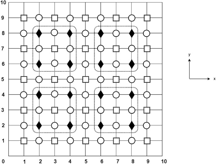
Figure 1. Distribution of mesh points of the LMFEGM with $M_x=M_y=10$.

Here, $D_1$, $D_2$, $D_3$, $D_4$, and $D_5$ are grid functions, which are defined as follows:

$\begin{array}{ll}\hfill D_1^{i,j}& =1+\frac{\nu m}{4h_x^2}+\frac{\nu m}{4h_y^2}+\frac{m}{8h_x}\left(W_{i+2,j}^n-W_{i-2,j}^n\right)+\frac{m}{8h_y}\left(W_{i,j+2}^n-W_{i,j-2}^n\right),\hfill \\ \hfill D_2^{i,j}& =\frac{\nu m}{8h_x^2}-\frac{m}{8h_x}{W}_{i,j}^n,D_3^{i,j}=\frac{\nu m}{8h_x^2}+\frac{m}{8h_x}{W}_{i,j}^n,\hfill \\ \hfill D_4^{i,j}& =\frac{\nu m}{8h_y^2}-\frac{m}{8h_y}{W}_{i,j}^n,D_5^{i,j}=\frac{\nu m}{8h_y^2}+\frac{m}{8h_y}{W}_{i,j}^n.\hfill \end{array}$

By inverting the coefficient matrix in Equation 15, the linear system can be rewritten as follows:

$\left(\begin{array}{c}\hfill W_{i,j}^{n+1}\hfill \\ \hfill W_{i+2,j}^{n+1}\hfill \\ \hfill W_{i+2,j+2}^{n+1}\hfill \\ \hfill W_{i,j+2}^{n+1}\hfill \end{array}\right)=\frac{1}{S}\left(\begin{array}{cccc}\hfill S_1\hfill & \hfill S_2\hfill & \hfill S_3\hfill & \hfill S_4\hfill \\ \hfill S_5\hfill & \hfill S_6\hfill & \hfill S_7\hfill & \hfill S_8\hfill \\ \hfill S_9\hfill & \hfill S_{10}\hfill & \hfill S_{11}\hfill & \hfill S_{12}\hfill \\ \hfill S_{13}\hfill & \hfill S_{14}\hfill & \hfill S_{15}\hfill & \hfill S_{16}\hfill \end{array}\right)\left(\begin{array}{c}\hfill rh{s}_{i,j}\hfill \\ \hfill rh{s}_{i+2,j}\hfill \\ \hfill rh{s}_{i+2,j+2}\hfill \\ \hfill rh{s}_{i,j+2}\hfill \end{array}\right),(16)$

where

$\begin{array}{ll}\hfill S& =D_1^{i,j}{D}_1^{i+2,j}{D}_1^{i+2,j+2}{D}_1^{i,j+2}-D_1^{i,j}{D}_1^{i+2,j}{D}_3^{i+2,j+2}{D}_2^{i,j+2}\hfill \\ \hfill & -D_1^{i,j}{D}_4^{i+2,j}{D}_5^{i+2,j+2}{D}_1^{i,j+2}-D_2^{i,j}{D}_3^{i+2,j}{D}_1^{i+2,j+2}{D}_1^{i,j+2}\hfill \\ \hfill & +D_2^{i,j}{D}_3^{i+2,j}{D}_3^{i+2,j+2}{D}_2^{i,j+2}-D_2^{i,j}{D}_4^{i+2,j}{D}_3^{i+2,j+2}{D}_5^{i,j+2}\hfill \\ \hfill & -D_4^{i,j}{D}_1^{i+2,j}{D}_1^{i+2,j+2}{D}_5^{i,j+2}-D_4^{i,j}{D}_3^{i+2,j}{D}_5^{i+2,j+2}{D}_2^{i,j+2}\hfill \\ \hfill & +D_4^{i,j}{D}_4^{i+2,j}{D}_5^{i+2,j+2}{D}_5^{i,j+2},\hfill \\ \hfill S_1& =D_1^{i+2,j}{D}_1^{i+2,j+2}{D}_1^{i,j+2}-D_1^{i+2,j}{D}_3^{i+2,j+2}{D}_2^{i,j+2}-D_4^{i+2,j}{D}_5^{i+2,j+2}{D}_1^{i,j+2},\hfill \\ \hfill S_2& =D_2^{i,j}{D}_1^{i+2,j+2}{D}_1^{i,j+2}-D_2^{i,j}{D}_3^{i+2,j+2}{D}_2^{i,j+2}+D_4^{i,j}{D}_5^{i+2,j+2}{D}_2^{i,j+2},\hfill \\ \hfill S_3& =D_2^{i,j}{D}_4^{i+2,j}{D}_1^{i,j+2}+D_4^{i,j}{D}_1^{i+2,j}{D}_2^{i,j+2},\hfill \\ \hfill S_4& =D_2^{i,j}{D}_4^{i+2,j}{D}_3^{i+2,j+2}+D_4^{i,j}{D}_1^{i+2,j}{D}_1^{i+2,j+2}-D_4^{i,j}{D}_4^{i+2,j}{D}_5^{i+2,j+2},\hfill \\ \hfill S_5& =D_3^{i+2,j}{D}_1^{i+2,j+2}{D}_1^{i,j+2}-D_3^{i+2,j}{D}_3^{i+2,j+2}{D}_2^{i,j+2}+D_4^{i+2,j}{D}_3^{i+2,j+2}{D}_5^{i,j+2},\hfill \\ \hfill S_6& =D_1^{i,j}{D}_1^{i+2,j+2}{D}_1^{i,j+2}-D_1^{i,j}{D}_3^{i+2,j+2}{D}_2^{i,j+2}-D_4^{i,j}{D}_1^{i+2,j+2}{D}_5^{i,j+2},\hfill \\ \hfill S_7& =D_1^{i,j}{D}_4^{i+2,j}{D}_1^{i,j+2}+D_4^{i,j}{D}_3^{i+2,j}{D}_2^{i,j+2}-D_4^{i,j}{D}_4^{i+2,j}{D}_5^{i,j+2},\hfill \\ \hfill S_8& =D_1^{i,j}{D}_4^{i+2,j}{D}_3^{i+2,j+2}+D_4^{i,j}{D}_3^{i+2,j}{D}_1^{i+2,j+2},\hfill \\ \hfill S_9& =D_1^{i+2,j}{D}_3^{i+2,j+2}{D}_5^{i,j+2}+D_3^{i+2,j}{D}_5^{i+2,j+2}{D}_1^{i,j+2},\hfill \\ \hfill S_{10}& =D_1^{i,j}{D}_5^{i+2,j+2}{D}_1^{i,j+2}+D_2^{i,j}{D}_3^{i+2,j+2}{D}_5^{i,j+2}-D_4^{i,j}{D}_5^{i+2,j+2}{D}_5^{i,j+2},\hfill \\ \hfill S_{11}& =D_1^{i,j}{D}_1^{i+2,j}{D}_1^{i,j+2}-D_2^{i,j}{D}_3^{i+2,j}{D}_1^{i,j+2}-D_4^{i,j}{D}_1^{i+2,j}{D}_5^{i,j+2},\hfill \\ \hfill S_{12}& =D_1^{i,j}{D}_1^{i+2,j}{D}_3^{i+2,j+2}-D_2^{i,j}{D}_3^{i+2,j}{D}_3^{i+2,j+2}+D_4^{i,j}{D}_3^{i+2,j}{D}_5^{i+2,j+2},\hfill \\ \hfill S_{13}& =D_1^{i+2,j}{D}_1^{i+2,j+2}{D}_5^{i,j+2}+D_3^{i+2,j}{D}_5^{i+2,j+2}{D}_2^{i,j+2}-D_4^{i+2,j}{D}_5^{i+2,j+2}{D}_5^{i,j+2},\hfill \\ \hfill S_{14}& =D_1^{i,j}{D}_5^{i+2,j+2}{D}_2^{i,j+2}+D_2^{i,j}{D}_1^{i+2,j+2}{D}_5^{i,j+2},\hfill \\ \hfill S_{15}& =D_1^{i,j}{D}_1^{i+2,j}{D}_2^{i,j+2}-D_2^{i,j}{D}_3^{i+2,j}{D}_2^{i,j+2}+D_2^{i,j}{D}_4^{i+2,j}{D}_5^{i,j+2},\hfill \\ \hfill S_{16}& =D_1^{i,j}{D}_1^{i+2,j}{D}_1^{i+2,j+2}-D_1^{i,j}{D}_4^{i+2,j}{D}_5^{i+2,j+2}-D_2^{i,j}{D}_3^{i+2,j}{D}_1^{i+2,j+2},\hfill \end{array}$

and

$\begin{array}{ll}\hfill rh{s}_{i,j}& =\left(\frac{\nu m}{8h_x^2}+\frac{m}{8h_x}{W}_{i,j}^n\right)W_{i-2,j}^{n+1}+\left(\frac{\nu m}{8h_y^2}+\frac{m}{8h_y}{W}_{i,j}^n\right)W_{i,j-2}^{n+1}\hfill \\ \hfill & +\frac{\nu m}{8h_x^2}\left(W_{i+2,j}^n+W_{i-2,j}^n\right)+\frac{\nu m}{8h_y^2}\left(W_{i,j+2}^n+W_{i,j-2}^n\right)\hfill \\ \hfill & +\left(1-2^{1-\alpha }{\eta }_1-\frac{\nu m}{8h_x^2}-\frac{\nu m}{8h_y^2}\right)W_{i,j}^n+2^{1-\alpha }{\displaystyle \sum _{s=1}^{n-1}}\left({\eta }_{n-s}-{\eta }_{n-s+1}\right)W_{i,j}^s\hfill \\ \hfill & +2^{1-\alpha }{\eta }_n{W}_{i,j}^0+m{f}_{i,j}^{n+1/2},\hfill \\ \hfill rh{s}_{i+2,j}& =\left(\frac{\nu m}{8h_x^2}-\frac{m}{8h_x}{W}_{i+2,j}^n\right)W_{i+4,j}^{n+1}+\left(\frac{\nu m}{8h_y^2}+\frac{m}{8h_y}{W}_{i+2,j}^n\right)W_{i+2,j-2}^{n+1}\hfill \\ \hfill & +\frac{\nu m}{8h_x^2}\left(W_{i+4,j}^n+W_{i,j}^n\right)+\frac{\nu m}{8h_y^2}\left(W_{i+2,j+2}^n+W_{i+2,j-2}^n\right)\hfill \\ \hfill & +\left(1-2^{1-\alpha }{\eta }_1-\frac{\nu m}{8h_x^2}-\frac{\nu m}{8h_y^2}\right)W_{i+2,j}^n+2^{1-\alpha }{\displaystyle \sum _{s=1}^{n-1}}\left({\eta }_{n-s}-{\eta }_{n-s+1}\right)W_{i+2,j}^s\hfill \\ \hfill & +2^{1-\alpha }{\eta }_n{W}_{i+2,j}^0+m{f}_{i+2,j}^{n+1/2},\hfill \\ \hfill rh{s}_{i+2,j+2}& =\left(\frac{\nu m}{8h_x^2}-\frac{m}{8h_x}{W}_{i+2,j+2}^n\right)W_{i+4,j+2}^{n+1}+\left(\frac{\nu m}{8h_y^2}-\frac{m}{8h_y}{W}_{i+2,j+2}^n\right)W_{i+2,j+4}^{n+1}\hfill \\ \hfill & +\frac{\nu m}{8h_x^2}\left(W_{i+4,j+2}^n+W_{i,j+2}^n\right)+\frac{\nu m}{8h_y^2}\left(W_{i+2,j+4}^n+W_{i+2,j}^n\right)\hfill \\ \hfill & +\left(1-2^{1-\alpha }{\eta }_1-\frac{\nu m}{8h_x^2}-\frac{\nu m}{8h_y^2}\right)W_{i+2,j+2}^n+2^{1-\alpha }{\displaystyle \sum _{s=1}^{n-1}}\left({\eta }_{n-s}-{\eta }_{n-s+1}\right)W_{i+2,j+2}^s\hfill \\ \hfill & +2^{1-\alpha }{\eta }_n{W}_{i+2,j+2}^0+m{f}_{i+2,j+2}^{n+1/2},\hfill \\ \hfill rh{s}_{i,j+2}& =\left(\frac{\nu m}{8h_x^2}+\frac{m}{8h_x}{W}_{i,j+2}^n\right)W_{i-2,j+2}^{n+1}+\left(\frac{\nu m}{8h_y^2}-\frac{m}{8h_y}{W}_{i,j+2}^n\right)W_{i,j+4}^{n+1}\hfill \\ \hfill & +\frac{\nu m}{8h_x^2}\left(W_{i+2,j+2}^n+W_{i-2,j+2}^n\right)+\frac{\nu m}{8h_y^2}\left(W_{i,j+4}^n+W_{i,j}^n\right)\hfill \\ \hfill & +\left(1-2^{1-\alpha }{\eta }_1-\frac{\nu m}{8h_x^2}-\frac{\nu m}{8h_y^2}\right)W_{i,j+2}^n+2^{1-\alpha }{\displaystyle \sum _{s=1}^{n-1}}\left({\eta }_{n-s}-{\eta }_{n-s+1}\right)W_{i,j+2}^s\hfill \\ \hfill & +2^{1-\alpha }{\eta }_n{W}_{i,j+2}^0+m{f}_{i,j+2}^{n+1/2}.\hfill \end{array}$

For the sake of the numerical implementation of the LMFEGM, we derive a new linearized difference scheme for the considered problem (Equation 2). To this end, we consider a skewed mesh designed by rotating the standard mesh 45$°$ clockwise. Applying Taylor series expansion on the skewed mesh for spatial derivatives and utilizing Equation 7 for the fractional temporal derivative, we obtain the following:

$\begin{array}{cc}\hfill & \sigma \left[{\eta }_1{w}_{i,j}^n+{\displaystyle \sum _{s=1}^{n-1}}\left({\eta }_{n-s+1}-{\eta }_{n-s}\right)w_{i,j}^s-{\eta }_n{w}_{i,j}^0+\frac{\left(w_{i,j}^{n+1}-w_{i,j}^n\right)}{2^{1-\alpha }}\right]\hfill \\ \hfill & -\frac{\nu }{2}\left[\frac{w_{i+1,j-1}^{n+1}-2w_{i,j}^{n+1}+w_{i-1,j+1}^{n+1}}{2h_x^2}+\frac{w_{i+1,j-1}^n-2w_{i,j}^n+w_{i-1,j+1}^n}{2h_x^2}\right]\hfill \\ \hfill & -\frac{\nu }{2}\left[\frac{w_{i+1,j+1}^{n+1}-2w_{i,j}^{n+1}+w_{i-1,j-1}^{n+1}}{2h_y^2}+\frac{w_{i+1,j+1}^n-2w_{i,j}^n+w_{i-1,j-1}^n}{2h_y^2}\right]\hfill \\ \hfill & +\frac{1}{8h_x}\left[w_{i,j}^n\left(w_{i+1,j+1}^{n+1}-w_{i-1,j-1}^{n+1}+w_{i+1,j-1}^{n+1}-w_{i-1,j+1}^{n+1}\right)+w_{i,j}^{n+1}\left(w_{i+1,j+1}^n\right.\right.\hfill \\ \hfill & \left.\left.-w_{i-1,j-1}^n+w_{i+1,j-1}^n-w_{i-1,j+1}^n\right)\right]+\frac{1}{8h_y}\left[w_{i,j}^n\left(w_{i+1,j+1}^{n+1}-w_{i-1,j-1}^{n+1}\right.\right.\hfill \\ \hfill & \left.\left.+w_{i-1,j+1}^{n+1}-w_{i+1,j-1}^{n+1}\right)+w_{i,j}^{n+1}\left(w_{i+1,j+1}^n-w_{i-1,j-1}^n+w_{i-1,j+1}^n-w_{i+1,j-1}^n\right)\right]\hfill \\ \hfill & =f_{i,j}^{n+1/2}+O\left({\left(\mathrm{\Delta }t\right)}^{2-\alpha }+{\left(\mathrm{\Delta }x\right)}^2+{\left(\mathrm{\Delta }y\right)}^2\right).\hfill \end{array}$

After rearrangement and omission of the higher-order small error terms, the following linearized skewed difference method (LSDM) is obtained:

$\begin{array}{cc}\hfill & \left(1+\frac{\nu m}{2h_x^2}+\frac{\nu m}{2h_y^2}+\frac{m}{8h_x}\left(W_{i+1,j+1}^n-W_{i-1,j-1}^n+W_{i+1,j-1}^n-W_{i-1,j+1}^n\right)\right.\hfill \\ \hfill & \left.+\frac{m}{8h_y}\left(W_{i+1,j+1}^n-W_{i-1,j-1}^n+W_{i-1,j+1}^n-W_{i+1,j-1}^n\right)\right)W_{i,j}^{n+1}\hfill \\ \hfill & =\left(\frac{\nu m}{4h_x^2}-\frac{m}{8h_x}{W}_{i,j}^n+\frac{m}{8h_y}{W}_{i,j}^n\right)W_{i+1,j-1}^{n+1}+\left(\frac{\nu m}{4h_x^2}+\frac{m}{8h_x}{W}_{i,j}^n-\frac{m}{8h_y}{W}_{i,j}^n\right)W_{i-1,j+1}^{n+1}\hfill \\ \hfill & +\left(\frac{\nu m}{4h_y^2}-\frac{m}{8h_x}{W}_{i,j}^n-\frac{m}{8h_y}{W}_{i,j}^n\right)W_{i+1,j+1}^{n+1}+\left(\frac{\nu m}{4h_y^2}+\frac{m}{8h_x}{W}_{i,j}^n+\frac{m}{8h_y}{W}_{i,j}^n\right)W_{i-1,j-1}^{n+1}\hfill \\ \hfill & +\frac{\nu m}{4h_x^2}\left(W_{i+1,j-1}^n+W_{i-1,j+1}^n\right)+\frac{\nu m}{4h_y^2}\left(W_{i+1,j+1}^n+W_{i-1,j-1}^n\right)\hfill \\ \hfill & +\left(1-2^{1-\alpha }{\eta }_1-\frac{\nu m}{2h_x^2}-\frac{\nu m}{2h_y^2}\right)W_{i,j}^n+2^{1-\alpha }{\displaystyle \sum _{s=1}^{n-1}}\left({\eta }_{n-s}-{\eta }_{n-s+1}\right)W_{i,j}^s\hfill \\ \hfill & +2^{1-\alpha }{\eta }_n{W}_{i,j}^0+m{f}_{i,j}^{n+1/2},1\le i\le M_x-1,1\le j\le M_y-1,0\le n\le N-1.\hfill \end{array}$

Figure 1 shows the distribution of the mesh points for the LMFEGM. It can be observed that the mesh points are divided into three types, denoted by $⧫$, □, and ○. The implementation of the LMFEGM comprises the computation of the solution values at $⧫$ points iteratively using Equation 16. After convergence is achieved, the solution values at the remaining □ and ○ points are computed directly using the LSDM (Equation 17) and LCNDM (Equation 11), respectively. The evaluated solution values are then used as the initial guess for the next time level, and the described solution process continues until the targeted time level is reached. Numerical implementation and comprehensive comparison between the LCNDM and LMFEGM is provided in Section 7. Prior to that, the subsequent two sections are focus on the stability and convergence of the proposed methods.

4 Stability analysis

The stability of a numerical scheme guarantees that round-off errors do not amplify and remain bounded as the computation process progresses from one time level to the next. In this section, we analyze the stability of the proposed methods using the Fourier method. In this regard, it is advantageous to recall that the nonlinear convection term $w(w_x+w_y)$ has been linearized by replacing $w$ with a local constant $\bar{w}$. As a result, the model problem (Equation 2) now takes the following form:

${}_0{}^{C}D_t^{\alpha }w\left(\mathbf{x},t\right)-\nu \mathrm{\Delta }w\left(\mathbf{x},t\right)+\bar{w}\left(\mathbf{x},t\right)\left(\nabla w\left(\mathbf{x},t\right)\cdot \mathbf{1}\right)=f\left(\mathbf{x},t\right).$

For stability analysis, we linearize the nonlinear term $w(x_x+w_y)$ by regarding $w$ as a locally constant function $\bar{w}$. This simplification allows us to apply Fourier techniques but assumes that $\bar{w}$ is invariant in space and time during the analysis. We emphasize that this is a theoretical construct for proving stability; numerical experiments in Section 6 confirm that the methods remain robust under the actual variable system. For strongly nonlinear regimes, other techniques can be used.

For later uses, the following lemma is introduced:

Lemma 1. For the coefficients ${\eta }_s,(s=\mathrm{0,1},\dots )$ in Equation 7, it holds that

1. ${\eta }_{n-s}>{\eta }_{n-s+1},s=\mathrm{0,1,2},\dots ,n-1$, and

2. ${\sum }_{s=1}^{n-1}\left({\eta }_{n-s}-{\eta }_{n-s+1}\right)={\eta }_1-{\eta }_n$.

4.1 Stability of the $h$-spaced linearized difference scheme

To prove the stability of the $h$-spaced linearized difference scheme (Equation 9), we need some notations. Let $\tilde{W}=\{{\tilde{W}}_{i,j}^n|1\le i\le M_x-1,1\le j\le M_y-1,0\le n\le N-1\}$ be the approximate solution of the discrete scheme (Equation 9). The round-off error is defined as

${\zeta }_{i,j}^n=W_{i,j}^n-{\tilde{W}}_{i,j}^n,1\le i\le M_x-1,1\le j\le M_y-1,0\le n\le N-1.(17)$

Substituting Equation 17 into Equation 9 leads to the following round-off error equation:

$\begin{array}{cc}\hfill & \left(1+\frac{\nu m}{{\left(\mathrm{\Delta }x\right)}^2}+\frac{\nu m}{{\left(\mathrm{\Delta }y\right)}^2}\right){\zeta }_{i,j}^{n+1}-\left(\frac{\nu m}{2{\left(\mathrm{\Delta }x\right)}^2}-\frac{m}{4\mathrm{\Delta }x}\bar{w}\right){\zeta }_{i+1,j}^{n+1}\hfill \\ \hfill & -\left(\frac{\nu m}{2{\left(\mathrm{\Delta }x\right)}^2}+\frac{m}{4\mathrm{\Delta }x}\bar{w}\right){\zeta }_{i-1,j}^{n+1}-\left(\frac{\nu m}{2{\left(\mathrm{\Delta }y\right)}^2}-\frac{m}{4\mathrm{\Delta }y}\bar{w}\right){\zeta }_{i,j+1}^{n+1}\hfill \\ \hfill & -\left(\frac{\nu m}{2{\left(\mathrm{\Delta }y\right)}^2}+\frac{m}{4\mathrm{\Delta }y}\bar{w}\right){\zeta }_{i,j-1}^{n+1}=\left(\frac{\nu m}{2{\left(\mathrm{\Delta }x\right)}^2}-\frac{m}{4\mathrm{\Delta }x}\bar{w}\right){\zeta }_{i+1,j}^n\hfill \\ \hfill & +\left(\frac{\nu m}{2{\left(\mathrm{\Delta }x\right)}^2}+\frac{m}{4\mathrm{\Delta }x}\bar{w}\right){\zeta }_{i-1,j}^n+\left(\frac{\nu m}{2{\left(\mathrm{\Delta }y\right)}^2}-\frac{m}{4\mathrm{\Delta }y}\bar{w}\right){\zeta }_{i,j+1}^n\hfill \\ \hfill & +\left(\frac{\nu m}{2{\left(\mathrm{\Delta }y\right)}^2}+\frac{m}{4\mathrm{\Delta }y}\bar{w}\right){\zeta }_{i,j-1}^n+\left(1-2^{1-\alpha }{\eta }_1-\frac{\nu m}{{\left(\mathrm{\Delta }x\right)}^2}-\frac{\nu m}{{\left(\mathrm{\Delta }y\right)}^2}\right){\zeta }_{i,j}^n\hfill \\ \hfill & +2^{1-\alpha }{\displaystyle \sum _{s=1}^{n-1}}\left({\eta }_{n-s}-{\eta }_{n-s+1}\right){\zeta }_{i,j}^s+2^{1-\alpha }{\eta }_n{\zeta }_{i,j}^0.\hfill \end{array}(18)$

Without loss of generality, we assume that $L_x=L_y=L$; then, the grid function ${\zeta }^n(\mathbf{x})$ is given by

${\zeta }^n\left(\mathbf{x}\right)=\left\{\begin{array}{cc}{\zeta }_{i,j}^n,\hfill & x_i-\frac{\mathrm{\Delta }x}{2}<x\le x_i+\frac{\mathrm{\Delta }x}{2},y_j-\frac{\mathrm{\Delta }y}{2}<y\le y_j+\frac{\mathrm{\Delta }y}{2},\hfill \\ 0,\hfill & 0\le x\le \frac{\mathrm{\Delta }x}{2}\text{\hspace{0.17em}or\hspace{0.17em}}L-\frac{\mathrm{\Delta }x}{2}<x\le L\text{,}\hfill \\ 0,\hfill & 0\le y\le \frac{\mathrm{\Delta }y}{2}\text{\hspace{0.17em}or\hspace{0.17em}}L-\frac{\mathrm{\Delta }y}{2}<y\le L\text{,}\hfill \end{array}\right.$

and its Fourier expansion is in the form:

$\begin{array}{c}\hfill {\zeta }^n\left(\mathbf{x}\right)={\displaystyle \sum _{q_1=-\infty }^{\infty }}{\displaystyle \sum _{q_2=-\infty }^{\infty }}{\mathrm{\Phi }}^n\left(q_1,q_2\right)e^{2\pi \sqrt{-1}\left(q_{1}x/L+q_{2}y/L\right)},\end{array}$

where

${\mathrm{\Phi }}^n\left(q_1,q_2\right)=\frac{1}{L}{\int }_0^L{\int }_0^L{\zeta }^n\left(x,y\right)e^{-2\pi \sqrt{-1}\left(q_{1}x/L+q_{2}y/L\right)}dxdy.$

From the $l_2$ norm definition,

$\Vert {\zeta }^n{\Vert }_2={\left({\displaystyle \sum _{j=1}^{M_y-1}}{\displaystyle \sum _{i=1}^{M_x-1}}\mathrm{\Delta }y\mathrm{\Delta }x|{\zeta }_{i,j}^n{|}^2\right)}^{1/2}={\left({\int }_0^L{\int }_0^L|{\zeta }_{i,j}^n{|}^{2}dxdy\right)}^{1/2}.$

Applying Parseval’s equality,

${\int }_0^L{\int }_0^L|{\zeta }_{i,j}^n{|}^{2}dxdy={\displaystyle \sum _{q_2=-\infty }^{\infty }}{\displaystyle \sum _{q_1=-\infty }^{\infty }}|{\mathrm{\Phi }}^n\left(q_1,q_2\right){|}^2,$

we obtain

$\begin{array}{c}\hfill \Vert {\zeta }^n{\Vert }_2={\left({\displaystyle \sum _{q_2=-\infty }^{\infty }}{\displaystyle \sum _{q_1=-\infty }^{\infty }}|{\mathrm{\Phi }}^n\left(q_1,q_2\right){|}^2\right)}^{1/2}.\end{array}(19)$

We can assume that the solution of $(24)$ is expressed as follows:

${\zeta }_{i,j}^n={\mathrm{\Phi }}^n{e}^{\sqrt{-1}\left({\theta }_{1}i\mathrm{\Delta }x+{\theta }_{2}j\mathrm{\Delta }y\right)},(20)$

where ${\theta }_1=2\pi q_1/L$ and ${\theta }_2=2\pi q_2/L$. Now, we prove the next result.

Lemma 2. For $0\le n\le N-1$, if $3^{1-\alpha }\le 2$, then it holds that $|{\mathrm{\Phi }}^{n+1}|\le |{\mathrm{\Phi }}^0|$.

Proof: Substituting Equation 20 into Equation 18 and carrying out simplifications lead to

$\begin{array}{cc}\hfill {\mathrm{\Phi }}^{n+1}& =\frac{1-\mu -2\sqrt{-1}\bar{w}\bar{\mu }-2^{1-\alpha }{\eta }_1}{1+\mu +2\sqrt{-1}\bar{w}\bar{\mu }}{\mathrm{\Phi }}^n\hfill \\ \hfill & +\frac{2^{1-\alpha }}{1+\mu +2\sqrt{-1}\bar{w}\bar{\mu }}\left[{\displaystyle \sum _{s=1}^{n-1}}\left({\eta }_{n-s}-{\eta }_{n-s+1}\right){\mathrm{\Phi }}^s+{\eta }_n{\mathrm{\Phi }}^0\right],\hfill \end{array}(21)$

where

$\begin{array}{ll}\hfill \mu & =\frac{2\nu m}{{\left(\mathrm{\Delta }x\right)}^2}{\sin }^2\left(\frac{{\theta }_1\mathrm{\Delta }x}{2}\right)+\frac{2\nu m}{{\left(\mathrm{\Delta }y\right)}^2}{\sin }^2\left(\frac{{\theta }_2\mathrm{\Delta }2}{2}\right),\hfill \\ \hfill \bar{\mu }& =\frac{m}{4\mathrm{\Delta }x}\sin \left({\theta }_1\mathrm{\Delta }x\right)+\frac{m}{4\mathrm{\Delta }y}\sin \left({\theta }_2\mathrm{\Delta }y\right).\hfill \end{array}$

By substituting $n=0$ in Equation 21 and since $\mu \ge 0$, we obtain

$|{\mathrm{\Phi }}^1|=\left|\frac{1-\mu -2\sqrt{-1}\bar{w}\bar{\mu }}{1+\mu +2\sqrt{-1}\bar{w}\bar{\mu }}\right|\left|{\mathrm{\Phi }}^0\right|=\sqrt{\frac{{\left(1-\mu \right)}^2+{\left(2\bar{w}\bar{\mu }\right)}^2}{{\left(1+\mu \right)}^2+{\left(2\bar{w}\bar{\mu }\right)}^2}}|{\mathrm{\Phi }}^0|\le |{\mathrm{\Phi }}^0|.$

Now, we assume that

$|{\mathrm{\Phi }}^{k+1}|\le |{\mathrm{\Phi }}^0|,0\le k\le n-1.(22)$

From Equation 21, Equation 22, and lemma 1, we obtain

$\begin{array}{ll}\hfill |{\mathrm{\Phi }}^{n+1}|& \le \left|\frac{1-\mu -2\sqrt{-1}\bar{w}\bar{\mu }-2^{1-\alpha }{\eta }_1}{1+\mu +2\sqrt{-1}\bar{w}\bar{\mu }}\right|\left|{\mathrm{\Phi }}^n\right|\hfill \\ \hfill & +\left|\frac{2^{1-\alpha }}{1+\mu +2\sqrt{-1}\bar{w}\bar{\mu }}\right|\left[{\displaystyle \sum _{s=1}^{n-1}}\left|\left({\eta }_{n-s}-{\eta }_{n-s+1}\right)\right|\left|{\mathrm{\Phi }}^s\right|+\left|{\eta }_n\right|\left|{\mathrm{\Phi }}^0\right|\right],\hfill \\ \hfill & \le \left|\frac{1-\mu -2\sqrt{-1}\bar{w}\bar{\mu }-2^{1-\alpha }{\eta }_1}{1+\mu +2\sqrt{-1}\bar{w}\bar{\mu }}\right|\left|{\mathrm{\Phi }}^0\right|\hfill \\ \hfill & +\left|\frac{2^{1-\alpha }}{1+\mu +2\sqrt{-1}\bar{w}\bar{\mu }}\right|\left[{\displaystyle \sum _{s=1}^{n-1}}\left({\eta }_{n-s}-{\eta }_{n-s+1}\right)|{\mathrm{\Phi }}^0|+{\eta }_n|{\mathrm{\Phi }}^0|\right],\hfill \\ \hfill & =\left|\frac{1-\mu -2\sqrt{-1}\bar{w}\bar{\mu }-2^{1-\alpha }{\eta }_1}{1+\mu +2\sqrt{-1}\bar{w}\bar{\mu }}\right|\left|{\mathrm{\Phi }}^0\right|\hfill \\ \hfill & +\left|\frac{2^{1-\alpha }}{1+\mu +2\sqrt{-1}\bar{w}\bar{\mu }}\right|\left[\left({\eta }_1-{\eta }_n\right)|{\mathrm{\Phi }}^0|+{\eta }_n|{\mathrm{\Phi }}^0|\right],\hfill \\ \hfill & =\frac{|1-\mu -2\sqrt{-1}\bar{w}\bar{\mu }-2^{1-\alpha }{\eta }_1|+2^{1-\alpha }{\eta }_1}{1+\mu +2\sqrt{-1}\bar{w}\bar{\mu }}|{\mathrm{\Phi }}^0|.\hfill \end{array}$

As $n$ increases, $\mathrm{\Delta }t$, $\mu$, and $\bar{\mu }$ approach 0, which yields

$|{\mathrm{\Phi }}^{n+1}|\le \left(\left|1-2^{1-\alpha }{\eta }_1\right|+2^{1-\alpha }{\eta }_1\right)|{\mathrm{\Phi }}^0|.$

If $1-2^{1-\alpha }{\eta }_1>0$, then

$|{\mathrm{\Phi }}^{n+1}|\le |{\mathrm{\Phi }}^0|.$

If $1-2^{1-\alpha }{\eta }_1\le 0$, then

$|{\mathrm{\Phi }}^{n+1}|\le \left(-1+2^{2-\alpha }{\eta }_1\right)|{\mathrm{\Phi }}^0|.$

In such a case,

$\begin{array}{ll}\hfill |{\mathrm{\Phi }}^{n+1}|& \le |{\mathrm{\Phi }}^0|\hfill \\ \hfill & \iff -1+2^{2-\alpha }{\eta }_1\le 1,\hfill \\ \hfill & \iff 3^{1-\alpha }\le 2.\hfill \end{array}$

Theorem 1. If $3^{1-\alpha }\le 2$, then the difference scheme (Equation 9) is stable.

Proof: By considering lemma 2 and applying Parseval’s equality, we obtain

$\begin{array}{ll}\hfill \Vert {\zeta }^n{\Vert }_2& ={\displaystyle \sum _{j=1}^{M_y-1}}{\displaystyle \sum _{i=1}^{M_x-1}}\mathrm{\Delta }y\mathrm{\Delta }x|{\zeta }_{i,j}^n{|}^2=\mathrm{\Delta }y\mathrm{\Delta }x{\displaystyle \sum _{j=1}^{M_y-1}}{\displaystyle \sum _{i=1}^{M_x-1}}{\left|{\mathrm{\Phi }}^n{e}^{I\left({\theta }_{1}i\mathrm{\Delta }x+{\theta }_{2}j\mathrm{\Delta }y\right)}\right|}^2\hfill \\ \hfill & =\mathrm{\Delta }y\mathrm{\Delta }x{\displaystyle \sum _{j=1}^{M_y-1}}{\displaystyle \sum _{i=1}^{M_x-1}}|{\mathrm{\Phi }}^n{|}^2\le \mathrm{\Delta }y\mathrm{\Delta }x{\displaystyle \sum _{j=1}^{M_y-1}}{\displaystyle \sum _{i=1}^{M_x-1}}|{\mathrm{\Phi }}^0{|}^2\hfill \\ \hfill & =\mathrm{\Delta }y\mathrm{\Delta }x{\displaystyle \sum _{j=1}^{M_y-1}}{\displaystyle \sum _{i=1}^{M_x-1}}{\left|{\mathrm{\Phi }}^0{e}^{I\left({\theta }_{1}i\mathrm{\Delta }x+{\theta }_{2}j\mathrm{\Delta }y\right)}\right|}^2=\Vert {\zeta }^0{\Vert }_2.\hfill \end{array}$

4.2 Stability of the $2h$-spaced linearized difference scheme

In this section, we examine the stability of the $2h$-spaced linearized difference scheme (Equation 14) and introduce some necessary notations. Let $\bar{W}=\{{\bar{W}}_{i,j}^n|1\le i\le M_x-1,1\le j\le M_y-1,0\le n\le N-1\}$ be the approximate solution of the discrete scheme (Equation 14). The round-off error is expressed as follows:

${\rho }_{i,j}^n=W_{i,j}^n-{\bar{W}}_{i,j}^n,1\le i\le M_x-1,1\le j\le M_y-1,0\le n\le N-1.(23)$

By substituting Equation 23 into Equation 14, we obtain the following round-off error equation:

$\begin{array}{cc}\hfill & \left(1+\frac{\nu m}{4h_x^2}+\frac{\nu m}{4h_y^2}\right){\rho }_{i,j}^{n+1}-\left(\frac{\nu m}{8h_x^2}-\frac{m}{8h_x}\bar{w}\right){\rho }_{i+2,j}^{n+1}\hfill \\ \hfill & -\left(\frac{\nu m}{8h_x^2}+\frac{m}{8h_x}\bar{w}\right){\rho }_{i-2,j}^{n+1}-\left(\frac{\nu m}{8h_y^2}-\frac{m}{8h_y}\bar{w}\right){\rho }_{i,j+2}^{n+1}\hfill \\ \hfill & -\left(\frac{\nu m}{8h_y^2}+\frac{m}{8h_y}\bar{w}\right){\rho }_{i,j-2}^{n+1}=\left(\frac{\nu m}{8h_x^2}-\frac{m}{8h_x}\bar{w}\right){\rho }_{i+2,j}^n\hfill \\ \hfill & +\left(\frac{\nu m}{8h_x^2}+\frac{m}{8h_x}\bar{w}\right){\rho }_{i-2,j}^n+\left(\frac{\nu m}{8h_y^2}-\frac{m}{8h_y}\bar{w}\right){\rho }_{i,j+2}^n\hfill \\ \hfill & +\left(\frac{\nu m}{8h_y^2}+\frac{m}{8h_y}\bar{w}\right){\rho }_{i,j-2}^n+\left(1-2^{1-\alpha }{\eta }_1-\frac{\nu m}{4h_x^2}-\frac{\nu m}{4h_y^2}\right){\rho }_{i,j}^n\hfill \\ \hfill & +2^{1-\alpha }{\displaystyle \sum _{s=1}^{n-1}}\left({\eta }_{n-s}-{\eta }_{n-s+1}\right){\rho }_{i,j}^s+2^{1-\alpha }{\eta }_n{\rho }_{i,j}^0.\hfill \end{array}(24)$

The grid function ${\rho }^n(\mathbf{x})$ can be defined as in the previous subsection, while its Fourier expansion is given by

$\begin{array}{c}\hfill {\rho }^n\left(\mathbf{x}\right)={\displaystyle \sum _{q_1=-\infty }^{\infty }}{\displaystyle \sum _{q_2=-\infty }^{\infty }}{\mathrm{\Psi }}^n\left(q_1,q_2\right)e^{2\pi \sqrt{-1}\left(q_{1}x/L+q_{2}y/L\right)},\end{array}$

where

${\mathrm{\Psi }}^n\left(q_1,q_2\right)=\frac{1}{L}{\int }_0^L{\int }_0^L{\rho }^n\left(\mathbf{x}\right)e^{-2\pi \sqrt{-1}\left(q_{1}x/L+q_{2}y/L\right)}dxdy.$

The $l_2$ norm definition provides

$\Vert {\rho }^n{\Vert }_2={\left({\displaystyle \sum _{j=1}^{M_y-1}}{\displaystyle \sum _{i=1}^{M_x-1}}\mathrm{\Delta }y\mathrm{\Delta }x|{\rho }_{i,j}^n{|}^2\right)}^{1/2}={\left({\int }_0^L{\int }_0^L|{\rho }_{i,j}^n{|}^{2}dxdy\right)}^{1/2}.$

Applying Parseval’s equality,

${\int }_0^L{\int }_0^L|{\rho }_{i,j}^n{|}^{2}dxdy={\displaystyle \sum _{q_2=-\infty }^{\infty }}{\displaystyle \sum _{q_1=-\infty }^{\infty }}|{\mathrm{\Psi }}^n\left(q_1,q_2\right){|}^2,$

we obtain

$\begin{array}{c}\hfill \Vert {\rho }^n{\Vert }_2={\left({\displaystyle \sum _{q_2=-\infty }^{\infty }}{\displaystyle \sum _{q_1=-\infty }^{\infty }}|{\mathrm{\Psi }}^n\left(q_1,q_2\right){|}^2\right)}^{1/2}.\end{array}$

Again, we can assume that the solution of Equation 29 is expressed as follows:

${\rho }_{i,j}^n={\mathrm{\Psi }}^n{e}^{\sqrt{-1}\left({\theta }_{1}i\mathrm{\Delta }x+{\theta }_{2}j\mathrm{\Delta }y\right)},(25)$

which leads us to the next result.

Lemma 3. For $0\le n\le N-1$, if $3^{1-\alpha }\le 2$, it holds that $|{\mathrm{\Psi }}^{n+1}|\le |{\mathrm{\Psi }}^0|$.

Proof: Substituting Equation 25 into Equation 24 and performing some rearrangements lead to

$\begin{array}{cc}\hfill {\mathrm{\Psi }}^{n+1}& =\frac{1-\lambda -2\sqrt{-1}\bar{w}\bar{\lambda }-2^{1-\alpha }{\eta }_1}{1+\lambda +2\sqrt{-1}\bar{w}\bar{\lambda }}{\mathrm{\Psi }}^n\hfill \\ \hfill & +\frac{2^{1-\alpha }}{1+\lambda +2\sqrt{-1}\bar{w}\bar{\lambda }}\left[{\displaystyle \sum _{s=1}^{n-1}}\left({\eta }_{n-s}-{\eta }_{n-s+1}\right){\mathrm{\Psi }}^s+{\eta }_n{\mathrm{\Psi }}^0\right],\hfill \end{array}(26)$

where

$\begin{array}{ll}\hfill \lambda & =\frac{\nu m}{2h_x^2}{\sin }^2\left({\theta }_1\mathrm{\Delta }x\right)+\frac{\nu m}{2h_y^2}{\sin }^2\left({\theta }_2\mathrm{\Delta }y\right),\hfill \\ \hfill \bar{\lambda }& =\frac{m}{8h_x}\sin \left(2{\theta }_1\mathrm{\Delta }x\right)+\frac{m}{8\mathrm{\Delta }y}\sin \left(2{\theta }_2\mathrm{\Delta }y\right).\hfill \end{array}$

Substituting $n=0$ in Equation 26 and since $\lambda \ge 0$, we obtain

$|{\mathrm{\Psi }}^1|=\left|\frac{1-\lambda -2\sqrt{-1}\bar{w}\bar{\lambda }}{1+\lambda +2\sqrt{-1}\bar{w}\bar{\lambda }}\right|\left|{\mathrm{\Psi }}^0\right|=\sqrt{\frac{{\left(1-\lambda \right)}^2+{\left(2\bar{w}\bar{\lambda }\right)}^2}{{\left(1+\lambda \right)}^2+{\left(2\bar{w}\bar{\lambda }\right)}^2}}|{\mathrm{\Psi }}^0|\le |{\mathrm{\Psi }}^0|.$

Now, we assume that

$|{\mathrm{\Psi }}^{k+1}|\le |{\mathrm{\Psi }}^0|,0\le k\le n-1.(27)$

From Equations 26, 27 and lemma 1, we obtain

$\begin{array}{ll}\hfill |{\mathrm{\Psi }}^{n+1}|& \le \left|\frac{1-\lambda -2\sqrt{-1}\bar{w}\bar{\lambda }-2^{1-\alpha }{\eta }_1}{1+\lambda +2\sqrt{-1}\bar{w}\bar{\lambda }}\right|\left|{\mathrm{\Psi }}^n\right|\hfill \\ \hfill & +\left|\frac{2^{1-\alpha }}{1+\lambda +2\sqrt{-1}\bar{w}\bar{\lambda }}\right|\left[{\displaystyle \sum _{s=1}^{n-1}}\left|\left({\eta }_{n-s}-{\eta }_{n-s+1}\right)\right|\left|{\mathrm{\Psi }}^s\right|+\left|{\eta }_n\right|\left|{\mathrm{\Psi }}^0\right|\right],\hfill \\ \hfill & \le \left|\frac{1-\lambda -2\sqrt{-1}\bar{w}\bar{\lambda }-2^{1-\alpha }{\eta }_1}{1+\lambda +2\sqrt{-1}\bar{w}\bar{\lambda }}\right|\left|{\mathrm{\Psi }}^0\right|\hfill \\ \hfill & +\left|\frac{2^{1-\alpha }}{1+\lambda +2\sqrt{-1}\bar{w}\bar{\lambda }}\right|\left[{\displaystyle \sum _{s=1}^{n-1}}\left({\eta }_{n-s}-{\eta }_{n-s+1}\right)|{\mathrm{\Psi }}^0|+{\eta }_n|{\mathrm{\Psi }}^0|\right],\hfill \\ \hfill & =\left|\frac{1-\lambda -2\sqrt{-1}\bar{w}\bar{\lambda }-2^{1-\alpha }{\eta }_1}{1+\lambda +2\sqrt{-1}\bar{w}\bar{\lambda }}\right|\left|{\mathrm{\Psi }}^0\right|\hfill \\ \hfill & +\left|\frac{2^{1-\alpha }}{1+\lambda +2\sqrt{-1}\bar{w}\bar{\lambda }}\right|\left[\left({\eta }_1-{\eta }_n\right)|{\mathrm{\Psi }}^0|+{\eta }_n|{\mathrm{\Psi }}^0|\right],\hfill \\ \hfill & =\frac{|1-\lambda -2\sqrt{-1}\bar{w}\bar{\lambda }-2^{1-\alpha }{\eta }_1|+2^{1-\alpha }{\eta }_1}{1+\lambda +2\sqrt{-1}\bar{w}\bar{\lambda }}|{\mathrm{\Psi }}^0|.\hfill \end{array}$

As $n$ increases, $\mathrm{\Delta }t$, $\lambda$, and $\bar{\lambda }$ approach 0, which yields

$|{\mathrm{\Psi }}^{n+1}|\le \left(|1-2^{1-\alpha }{\eta }_1|+2^{1-\alpha }{\eta }_1\right)|{\mathrm{\Psi }}^0|.$

From lemma 2, it immediately follows that

$\begin{array}{ll}\hfill |{\mathrm{\Psi }}^{n+1}|& \le |{\mathrm{\Psi }}^0|\hfill \\ \hfill & \iff -1+2^{2-\alpha }{\eta }_1\le 1,\hfill \\ \hfill & \iff 3^{1-\alpha }\le 2.\hfill \end{array}$

Theorem 2. If $3^{1-\alpha }\le 2$, then the difference scheme (Equation 15) is stable.

Proof: By considering lemma 3 and applying Parseval’s equality, we obtain

$\begin{array}{ll}\hfill \Vert {\rho }^n{\Vert }_2& ={\displaystyle \sum _{j=1}^{M_y-1}}{\displaystyle \sum _{i=1}^{M_x-1}}\mathrm{\Delta }y\mathrm{\Delta }x|{\rho }_{i,j}^n{|}^2=\mathrm{\Delta }y\mathrm{\Delta }x{\displaystyle \sum _{j=1}^{M_y-1}}{\displaystyle \sum _{i=1}^{M_x-1}}{|{\mathrm{\Psi }}^n{e}^{I\left({\theta }_{1}i\mathrm{\Delta }x+{\theta }_{2}j\mathrm{\Delta }y\right)}|}^2\hfill \\ \hfill & =\mathrm{\Delta }y\mathrm{\Delta }x{\displaystyle \sum _{j=1}^{M_y-1}}{\displaystyle \sum _{i=1}^{M_x-1}}|{\mathrm{\Psi }}^n{|}^2\le \mathrm{\Delta }y\mathrm{\Delta }x{\displaystyle \sum _{j=1}^{M_y-1}}{\displaystyle \sum _{i=1}^{M_x-1}}|{\mathrm{\Psi }}^0{|}^2\hfill \\ \hfill & =\mathrm{\Delta }y\mathrm{\Delta }x{\displaystyle \sum _{j=1}^{M_y-1}}{\displaystyle \sum _{i=1}^{M_x-1}}{|{\mathrm{\Psi }}^0{e}^{I\left({\theta }_{1}i\mathrm{\Delta }x+{\theta }_{2}j\mathrm{\Delta }y\right)}|}^2=\Vert {\rho }^0{\Vert }_2.\hfill \end{array}$

5 Convergence analysis

In this section, we analyze the convergence of the difference scheme (Equation 9). Some preliminaries are introduced first to prove our final result. We start by subtracting Equation 9 from Equation 8, which results in the following error equation:

$\begin{array}{cc}\hfill & \left(1+\frac{\nu m}{{\left(\mathrm{\Delta }x\right)}^2}+\frac{\nu m}{{\left(\mathrm{\Delta }y\right)}^2}\right)E_{i,j}^{n+1}-\left(\frac{\nu m}{2{\left(\mathrm{\Delta }x\right)}^2}-\frac{m}{4\mathrm{\Delta }x}\bar{w}\right)E_{i+1,j}^{n+1}\hfill \\ \hfill & -\left(\frac{\nu m}{2{\left(\mathrm{\Delta }x\right)}^2}+\frac{m}{4\mathrm{\Delta }x}\bar{w}\right)E_{i-1,j}^{n+1}-\left(\frac{\nu m}{2{\left(\mathrm{\Delta }y\right)}^2}-\frac{m}{4\mathrm{\Delta }y}\bar{w}\right)E_{i,j+1}^{n+1}\hfill \\ \hfill & -\left(\frac{\nu m}{2{\left(\mathrm{\Delta }y\right)}^2}+\frac{m}{4\mathrm{\Delta }y}\bar{w}\right)E_{i,j-1}^{n+1}=\left(\frac{\nu m}{2{\left(\mathrm{\Delta }x\right)}^2}-\frac{m}{4\mathrm{\Delta }x}\bar{w}\right)E_{i+1,j}^n\hfill \\ \hfill & +\left(\frac{\nu m}{2{\left(\mathrm{\Delta }x\right)}^2}+\frac{m}{4\mathrm{\Delta }x}\bar{w}\right)E_{i-1,j}^n+\left(\frac{\nu m}{2{\left(\mathrm{\Delta }y\right)}^2}-\frac{m}{4\mathrm{\Delta }y}\bar{w}\right)E_{i,j+1}^n\hfill \\ \hfill & +\left(\frac{\nu m}{2{\left(\mathrm{\Delta }y\right)}^2}+\frac{m}{4\mathrm{\Delta }y}\bar{w}\right)E_{i,j-1}^n+\left(1-2^{1-\alpha }{\eta }_1-\frac{\nu m}{{\left(\mathrm{\Delta }x\right)}^2}-\frac{\nu m}{{\left(\mathrm{\Delta }y\right)}^2}\right)E_{i,j}^n\hfill \\ \hfill & +2^{1-\alpha }{\displaystyle \sum _{s=1}^{n-1}}\left({\eta }_{n-s}-{\eta }_{n-s+1}\right)E_{i,j}^s+2^{1-\alpha }{\eta }_n{E}_{i,j}^0+m{R}_{i,j}^{n+1/2},\hfill \end{array}(28)$

where $R_{i,j}^{n+1/2}$ denotes the local truncation error, and

$E_{i,j}^n=w\left(x_i,y_j,t_n\right)-W_{i,j}^n,1\le i\le M_x-1,1\le j\le M_y-1,1\le n\le N.$

Hereafter, $C$ will denote a generic positive constant that may vary from one location to another. For $0\le n\le N$, the grid functions $E^n(\mathbf{x})$ and $R^n(\mathbf{x})$ can be defined as follows:

$E^n\left(\mathbf{x}\right)=\left\{\begin{array}{cc}{E}_{i,j}^n,\hfill & x_i-\frac{\mathrm{\Delta }x}{2}<x\le x_i+\frac{\mathrm{\Delta }x}{2},y_j-\frac{\mathrm{\Delta }y}{2}<y\le y_j+\frac{\mathrm{\Delta }y}{2},\hfill \\ 0,\hfill & 0\le x\le \frac{\mathrm{\Delta }x}{2}\text{\hspace{0.17em}or\hspace{0.17em}}L-\frac{\mathrm{\Delta }x}{2}<x\le L\text{,}\hfill \\ 0,\hfill & 0\le y\le \frac{\mathrm{\Delta }y}{2}\text{\hspace{0.17em}or\hspace{0.17em}}L-\frac{\mathrm{\Delta }y}{2}<y\le L\text{,}\hfill \end{array}\right.$

and

$R^n\left(\mathbf{x}\right)=\left\{\begin{array}{cc}{R}_{i,j}^n,\hfill & x_i-\frac{\mathrm{\Delta }x}{2}<x\le x_i+\frac{\mathrm{\Delta }x}{2},y_j-\frac{\mathrm{\Delta }y}{2}<y\le y_j+\frac{\mathrm{\Delta }y}{2},\hfill \\ 0,\hfill & 0\le x\le \frac{\mathrm{\Delta }x}{2}\text{\hspace{0.17em}or\hspace{0.17em}}L-\frac{\mathrm{\Delta }x}{2}<x\le L\text{,}\hfill \\ 0,\hfill & 0\le y\le \frac{\mathrm{\Delta }y}{2}\text{\hspace{0.17em}or\hspace{0.17em}}L-\frac{\mathrm{\Delta }y}{2}<y\le L\text{.}\hfill \end{array}\right.$

The Fourier expansions of $E^n(\mathbf{x})$ and $R^n(\mathbf{x})$ can be written as follows:

$E^n\left(\mathbf{x}\right)={\displaystyle \sum _{q_2=-\infty }^{\infty }}{\displaystyle \sum _{q_1=-\infty }^{\infty }}{\mathrm{\Upsilon }}^n\left(q_1,q_2\right)e^{2\pi \sqrt{-1}\left(q_{1}x/L+q_{2}y/L\right)},$

$R^n\left(\mathbf{x}\right)={\displaystyle \sum _{q_2=-\infty }^{\infty }}{\displaystyle \sum _{q_1=-\infty }^{\infty }}{\mathrm{\Theta }}^n\left(q_1,q_2\right)e^{2\pi \sqrt{-1}\left(q_{1}x/L+q_{2}y/L\right)},$

where $\mathrm{\Upsilon }$ and $\mathrm{\Theta }$ are the Fourier coefficients, and the following norms are introduced:

$\Vert E^n{\Vert }_2^2={\displaystyle \sum _{i=1}^{M_x-1}}{\displaystyle \sum _{j=1}^{M_y-1}}\mathrm{\Delta }x\mathrm{\Delta }y|{E_{i,j}^n|}^2={\displaystyle \sum _{q_1=-\infty }^{\infty }}{\displaystyle \sum _{q_2=-\infty }^{\infty }}|{{\mathrm{\Upsilon }}^n\left(q_1,q_2\right)|}^2,0\le n\le N,(29)$

$\Vert R^n{\Vert }_2^2={\displaystyle \sum _{i=1}^{M_x-1}}{\displaystyle \sum _{j=1}^{M_y-1}}\mathrm{\Delta }x\mathrm{\Delta }y|{R_{i,j}^n|}^2={\displaystyle \sum _{q_1=-\infty }^{\infty }}{\displaystyle \sum _{q_2=-\infty }^{\infty }}|{{\mathrm{\Theta }}^n\left(q_1,q_2\right)|}^2,0\le n\le N.(30)$

It should be noted that from Equation 8, there exists a positive constant $C$such that

$|R_{i,j}^{n+1/2}|\le C\left({\left(\mathrm{\Delta }t\right)}^{2-\alpha }+{\left(\mathrm{\Delta }x\right)}^2+{\left(\mathrm{\Delta }y\right)}^2\right),1\le i\le M_x-1,1\le j\le M_y-1,0\le n\le N-1.$

In addition, from the convergence of the right-hand side of Equation 30, we can obtain a positive constant $C$ such that

$|{\mathrm{\Theta }}^{n+1/2}|\equiv |{\mathrm{\Theta }}^{n+1/2}\left(q_1,q_2\right)\le C|{\mathrm{\Theta }}^{1/2}\left(q_1,q_2\right)\equiv C|{\mathrm{\Theta }}^{1/2}|.(31)$

Prior to the next result, we now suppose that

$E_{i,j}^n={\mathrm{\Upsilon }}^n{e}^{I\left({\theta }_{1}i\mathrm{\Delta }x+{\theta }_{2}j\mathrm{\Delta }y\right)},R_{i,j}^n={\mathrm{\Theta }}^n{e}^{\sqrt{-1}\left({\theta }_{1}i\mathrm{\Delta }x+{\theta }_{2}j\mathrm{\Delta }y\right)}.(32)$

Lemma 4. For $0\le n\le N-1$, if $3^{1-\alpha }\le 2$, it holds that $|{\mathrm{\Upsilon }}^{n+1}|\le C|{\mathrm{\Theta }}^{1/2}|$.

Proof: Substituting Equation 31 into Equation 28 and simplifying yield

$\begin{array}{cc}\hfill {\mathrm{\Upsilon }}^{n+1}& =\frac{1-\mu -2\sqrt{-1}\bar{w}\bar{\mu }-2^{1-\alpha }{\eta }_1}{1+\mu +2\sqrt{-1}\bar{w}\bar{\mu }}{\mathrm{\Upsilon }}^n\hfill \\ \hfill & +\frac{1}{1+\mu +2\sqrt{-1}\bar{w}\bar{\mu }}\left[2^{1-\alpha }{\displaystyle \sum _{s=1}^{n-1}}\left({\eta }_{n-s}-{\eta }_{n-s+1}\right){\mathrm{\Upsilon }}^s+2^{1-\alpha }{\eta }_n{\mathrm{\Upsilon }}^0+m{\mathrm{\Theta }}^{n+1/2}\right],\hfill \end{array}(33)$

where $\mu$ and $\bar{\mu }$ are as defined before. For $n=0$ in Equation 33 and noting that ${\mathrm{\Upsilon }}^0\equiv {\mathrm{\Upsilon }}^0(q_1,q_2)=0$, we obtain

$|{\mathrm{\Upsilon }}^1|=|\frac{{\left(\mathrm{\Delta }t\right)}^{\alpha }}{1+\mu +2\sqrt{-1}\bar{w}\bar{\mu }}|2^{1-\alpha }\mathrm{\Gamma }\left(2-\alpha \right)|{\mathrm{\Theta }}^{1/2}|\le C|{\mathrm{\Theta }}^{1/2}|.$

Now, we assume that

$|{\mathrm{\Upsilon }}^k|\le C|{\mathrm{\Theta }}^{1/2}|,1\le k\le n.(34)$

From Equations 31, 33, 34 and lemma 1, we obtain

$\begin{array}{ll}\hfill |{\mathrm{\Upsilon }}^{n+1}|& \le \left|\frac{1-\mu -2\sqrt{-1}\bar{w}\bar{\mu }-2^{1-\alpha }{\eta }_1}{1+\mu +2\sqrt{-1}\bar{w}\bar{\mu }}\right|\left|{\mathrm{\Upsilon }}^n\right|\hfill \\ \hfill & +\left|\frac{1}{1+\mu 3+2\sqrt{-1}\bar{w}\bar{\mu }}\right|\left[2^{1-\alpha }{\displaystyle \sum _{s=1}^{n-1}}\left|\left({\eta }_{n-s}-{\eta }_{n-s+1}\right)\right|\left|{\mathrm{\Upsilon }}^s\right|+2^{1-\alpha }\left|{\eta }_n\right|\left|{\mathrm{\Upsilon }}^0\right|+m\left|{\mathrm{\Theta }}^{n+1/2}\right|\right],\hfill \\ \hfill & \le \left|\frac{1-\mu -2\sqrt{-1}\bar{w}\bar{\mu }-2^{1-\alpha }{\eta }_1}{1+\mu +2\sqrt{-1}\bar{w}\bar{\mu }}\right|C|{\mathrm{\Theta }}^{1/2}|\hfill \\ \hfill & +\left|\frac{1}{1+\mu +2\sqrt{-1}\bar{w}\bar{\mu }}\right|\left[2^{1-\alpha }{\displaystyle \sum _{s=1}^{n-1}}\left({\eta }_{n-s}-{\eta }_{n-s+1}\right)C|{\mathrm{\Theta }}^{1/2}|+2^{1-\alpha }{\eta }_{n}C|{\mathrm{\Theta }}^{1/2}|+mC|{\mathrm{\Theta }}^{1/2}|\right],\hfill \\ \hfill & =\left|\frac{1-\mu -2\sqrt{-1}\bar{w}\bar{\mu }-2^{1-\alpha }{\eta }_1}{1+\mu +2\sqrt{-1}\bar{w}\bar{\mu }}\right|C|{\mathrm{\Theta }}^{1/2}|\hfill \\ \hfill & +\left|\frac{1}{1+\mu +2\sqrt{-1}\bar{w}\bar{\mu }}\right|\left[2^{1-\alpha }\left({\eta }_1-{\eta }_n\right)C|{\mathrm{\Theta }}^{1/2}|+2^{1-\alpha }{\eta }_{n}C|{\mathrm{\Theta }}^{1/2}|+mC|{\mathrm{\Theta }}^{1/2}|\right],\hfill \\ \hfill & =\frac{|1-\mu -2\sqrt{-1}\bar{w}\bar{\mu }-2^{1-\alpha }{\eta }_1|+2^{1-\alpha }{\eta }_1+m}{|1+\mu +2\sqrt{-1}\bar{w}\bar{\mu }|}C|{\mathrm{\Theta }}^{1/2}|.\hfill \end{array}$

As $n$ increases, $\mathrm{\Delta }t$, $\mu$, $\bar{\mu }$, and $m$ approach 0, which yields

$|{\mathrm{\Upsilon }}^{n+1}|\le \left(|1-2^{1-\alpha }{\eta }_1|+2^{1-\alpha }{\eta }_1\right)C|{\mathrm{\Theta }}^{1/2}|.$

From lemma 2, we obtain

$\begin{array}{ll}\hfill |{\mathrm{\Upsilon }}^{n+1}|& \le C|{\mathrm{\Theta }}^{1/2}|\hfill \\ \hfill & \iff \left(|1-2^{1-\alpha }{\eta }_1|+2^{1-\alpha }{\eta }_1\right)\le 1,\hfill \\ \hfill & \iff 3^{1-\alpha }\le 2,\hfill \end{array}$

which completes the proof.

Theorem 3. The difference scheme (Equation 9) is $l_2$-convergent with a convergence order of $O({(\mathrm{\Delta }t)}^{2-\alpha }+{(\mathrm{\Delta }x)}^2+{(\mathrm{\Delta }y)}^2)$.

Proof: Using Equations 29, 30 and lemma 4, we obtain

$\begin{array}{ll}\hfill \Vert E^n{\Vert }_2^2& ={\displaystyle \sum _{j=1}^{M_y-1}}{\displaystyle \sum _{i=1}^{M_x-1}}\mathrm{\Delta }y\mathrm{\Delta }x|E_{i,j}^n{|}^2=\mathrm{\Delta }y\mathrm{\Delta }x{\displaystyle \sum _{j=1}^{M_y-1}}{\displaystyle \sum _{i=1}^{M_x-1}}{\left|{\mathrm{\Upsilon }}^n{e}^{\sqrt{-1}\left({\theta }_{1}i\mathrm{\Delta }x+{\theta }_{2}j\mathrm{\Delta }y\right)}\right|}^2\hfill \\ \hfill & =\mathrm{\Delta }y\mathrm{\Delta }x{\displaystyle \sum _{j=1}^{M_y-1}}{\displaystyle \sum _{i=1}^{M_x-1}}|{\mathrm{\Upsilon }}^n{|}^2\le C_2^2\mathrm{\Delta }y\mathrm{\Delta }x{\displaystyle \sum _{j=1}^{M_y-1}}{\displaystyle \sum _{i=1}^{M_x-1}}|{\mathrm{\Theta }}^{1/2}{|}^2\hfill \\ \hfill & =C_2^2\mathrm{\Delta }y\mathrm{\Delta }x{\displaystyle \sum _{j=1}^{M_y-1}}{\displaystyle \sum _{i=1}^{M_x-1}}{\left|{\mathrm{\Theta }}^{1/2}{e}^{\sqrt{-1}\left({\theta }_{1}i\mathrm{\Delta }x+{\theta }_{2}j\mathrm{\Delta }y\right)}\right|}^2=C_2^2\Vert R^{1/2}{\Vert }_2^2,\hfill \end{array}$

which completes the proof.

Theorem 4. The difference scheme (Equation 14) is $l_2$-convergent with a convergence order of $O({(\mathrm{\Delta }t)}^{2-\alpha }+{(\mathrm{\Delta }x)}^2+{(\mathrm{\Delta }y)}^2)$.

Proof: The proof can be established in a similar fashion to the proof of theorem 3.

It is worth pointing out that the discussions in Sections 4, 5 describe asymptotic stability and convergence analyses. A non-asymptotic analysis can be considered in future extensions of this work.

6 Numerical simulations and discussion of results

In this section, five numerical simulations corresponding to five test problems are carried out. The discussions are mainly based on the comparison of the numerical results for the LCNDM and LMFEGM in solving the time-fractional Burgers model. The maximum absolute error $MAE$ and CPU time (in seconds) of the aforementioned methods are selected to validate the accuracy and computational efficiency, respectively. We assume that $w(\mathbf{x},t)$ refers to the exact solution of the time-fractional Burgers model, ${\mathrm{w}\mathrm{h}\mathrm{e}\mathrm{r}\mathrm{e}\mathrm{a}\mathrm{s}}_{\mathit{LCNDM}}W$ ${\mathrm{a}\mathrm{n}\mathrm{d}}_{\mathit{LMFEGM}}W$ indicate the numerical solutions of the LCNDM and LMFEGM, respectively. The corresponding maximum absolute errors are computed using the following formulas:

$\begin{array}{ll}\hfill MA{E}_{\mathit{LCNDM}}& =\underset{1\le i\le M_{x-1},1\le j\le M_{y-1}}{\max }|w_{i,j}^N{-}_{\mathit{LCNDM}}{W}_{i,j}^N|,\hfill \\ \hfill MA{E}_{\mathit{LMFEGM}}& =\underset{1\le i\le M_{x-1},1\le j\le M_{y-1}}{\max }|w_{i,j}^N{-}_{\mathit{LMFEGM}}{W}_{i,j}^N|.\hfill \end{array}$

Based on the structure of the proposed methods, a new linearized system of equations needs to be solved at each time level. In this study, the proposed numerical schemes are combined with the Gauss–Seidel iterative solver to account for numerical results. In practice, the initial approximations are given by ${}_{LCNDM}W_{i,j}^{n,k}$ = ${}_{LCNDM}W_{i,j}^{n,k-1}$ and ${}_{LMFEGM}W_{i,j}^{n,k-1}$ = ${}_{\mathit{LMFEGM}}W_{i,j}^{n,k-1}$, where $k$ denotes the iteration’s number. In addition, the stopping criteria are set as $\Vert w^{n,k}{-}_{\mathit{LCNDM}}{W}^n{\Vert }_{\infty }\le 10^{-5}$ and $\Vert w^{n,k}{-}_{\mathit{LMFEGM}}{W}^n{\Vert }_{\infty }\le 10^{-5}$. Unless stated otherwise, the numerical results are obtained by considering $T=1$, $\mathrm{\Omega }=[\mathrm{0,1}]\times [\mathrm{0,1}]$, and $h_x=h_y=h=1/50$. All numerical simulations are performed using MATLAB R2018B on a Windows 64-bit system with an Intel(R) Core(TM) i7-8550 CPU and 8 GB of RAM.

Example 1. We consider the time-fractional Burgers model (Equations 2) with the following exact solution:

$w\left(\mathbf{x},t\right)=t^3{\left(1-x^2\right)}^2{\left(1-y^2\right)}^2.$

The initial and boundary conditions, in addition to the forcing term, can be extracted from the exact solution. The maximum error and CPU time of the LCNDM and LMFEGM, when the Reynolds number $(RE=1/\nu =10)$, in solving Example 1, are listed in Table 1. For different values of $\alpha$, it can be observed that both numerical methods converge well to the exact solution of the model problem. This is also apparent from Figure 2, which depicts the plots of the numerical and exact solutions when $h=1/70$, $N=50$, $\alpha =0.2$, and $RE=10$. On the other hand, it is also evident that the LMFEGM takes much less CPU time than the LCNDM in solving the considered problem. For instance, when $\alpha =0.1$ and $\mathrm{\Delta }t=0.02$, 46.90 s are required by the LCNDM, while only 3.78 s are needed by the LMFEGM for computing the numerical solutions.

Table 1

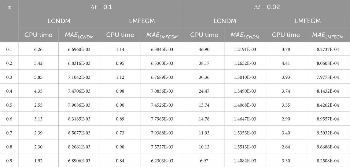
Table 1. Maximum error, iteration count, and CPU time obtained for Example 1 when $RE=10$.

Figure 2

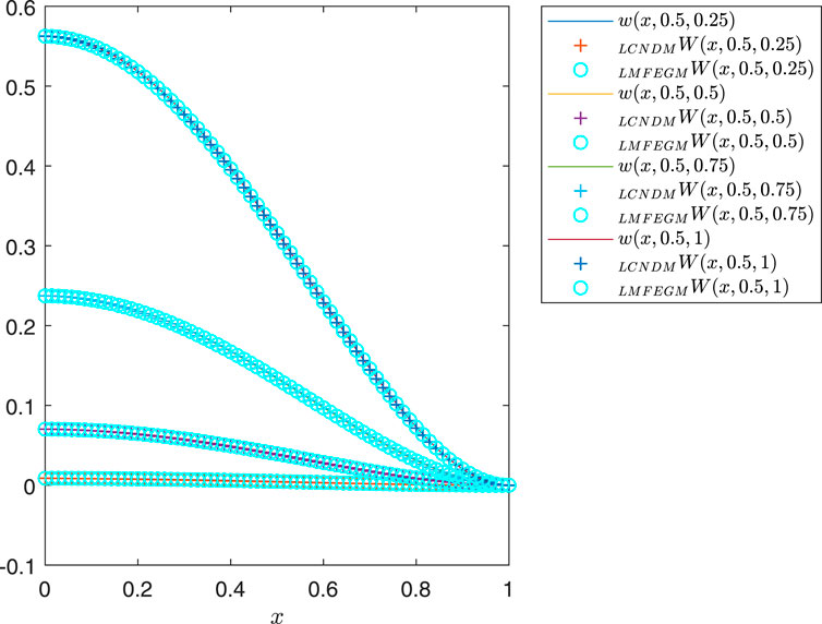
Figure 2. Graph of numerical and exact solutions for Example 1 with $T=1$, $h=1/70$, $N=50$, $\alpha =0.2$, and $RE=10$.

Example 2. We consider the time-fractional Burgers model (Equation 2) with the following exact solution:

$w\left(\mathbf{x},t\right)=t^3\cos \left(x\right)\cos \left(y\right).$

We solve this model problem subject to the initial and boundary conditions that can be drawn from the exact solution. The numerical results of the LCNDM and LMFEGM for the solution of Example 2, when $RE=30$, are recorded in Table 2, through which we can observe that decreasing values of $\mathrm{\Delta }t$ lead to better convergent solutions. The graph of the numerical and exact solutions for Example 2 when $T=1$, $h=1/70$, $N=50$, $\alpha =0.5$, and $RE=30$ is highlighted in Figure 3. Based on the data in these representations, there is no significant difference between the proposed methods in terms of accuracy; however, the LMFEGM converges much faster than the LCNDM, making it more efficient in solving the considered problem.

Table 2

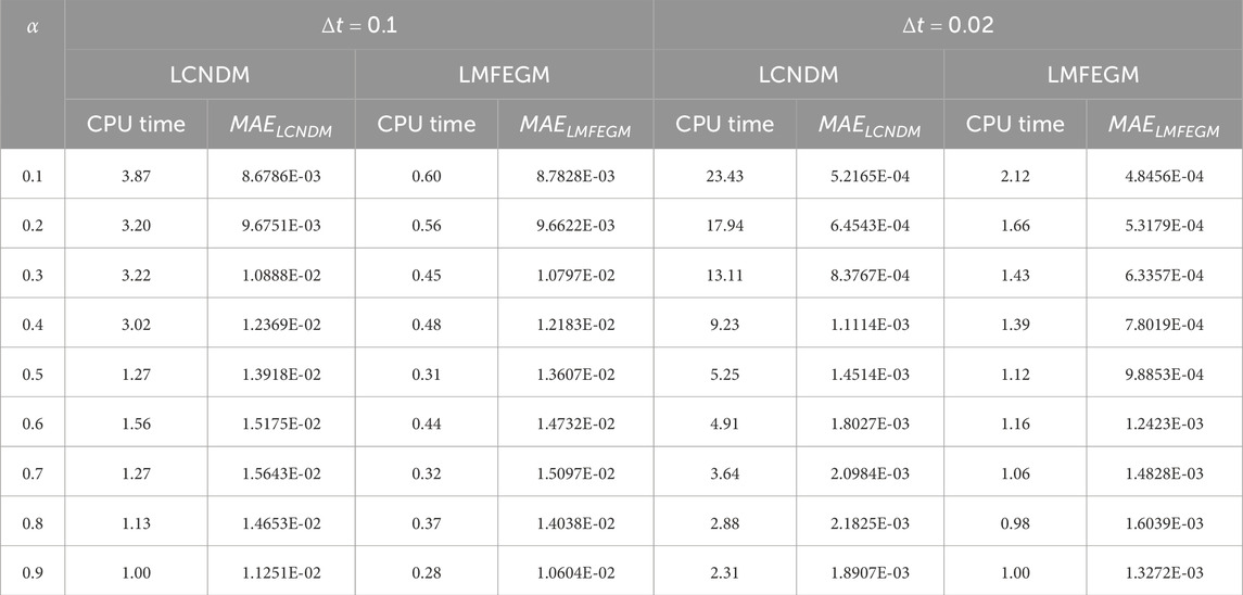
Table 2. Maximum error, iteration count, and CPU time obtained for Example 2 when $RE=30$.

Figure 3

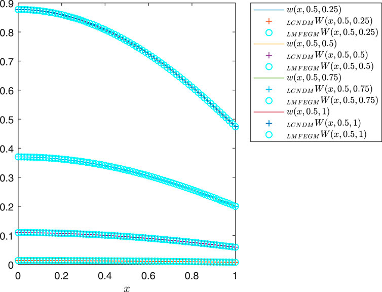
Figure 3. Graph of numerical and exact solutions for Example 1 with $T=1$, $h=1/70$, $N=50$, $\alpha =0.5$, and $RE=30$.

Example 3. Here, we consider the time-fractional Burgers model (Equation 2), which has the following exact solution:

$w\left(\mathbf{x},t\right)=t^2\left(x-x^2+y-y^2\right).$

Table 3 shows the numerical results in terms of maximum error and CPU time for Example 3 when $RE=70$. Figure 4 shows the sketch of the exact and numerical solutions for Example 3 when $T=1$, $h=1/70$, $N=50$, $\alpha =0.8$, and $RE=70$. Again, it can be observed that the numerical solutions of the proposed methods are compatible with the exact solution. In addition, the LMFEGM results in economic simulations since it requires less computational effort than the LCNDM. This illustrates that the LMFEGM is more efficient than the LCNDM when dealing with the time-fractional Burgers model.

Table 3

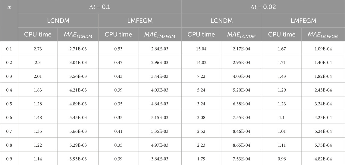
Table 3. Maximum error and CPU time obtained for Example 3 when $RE=70$.

Figure 4

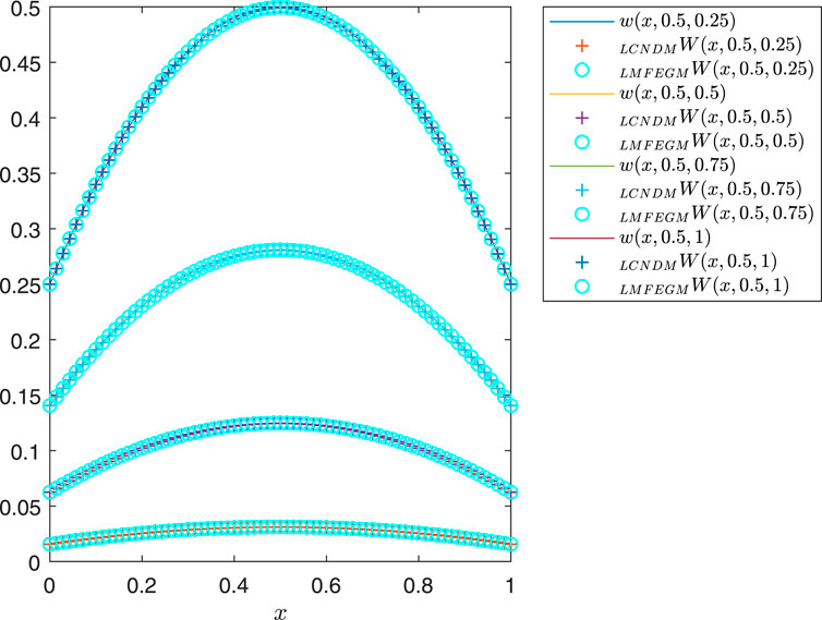
Figure 4. Graph of numerical and exact solutions for Example 1 with $T=1$, $h=1/70$, $N=50$, $\alpha =0.8$, and $RE=70$.

Example 4. We consider the time-fractional Burgers model (Equation 2) whose exact solution is in the following form:

$w\left(\mathbf{x},t\right)=\sin \left(t\right)\left(\sin \left(\pi x+\pi y\right)\right).$

Table 4 presents the computational outcomes for Example 4 at $\mathrm{R}\mathrm{e}=5$ with various values of fractional-order $\alpha$. From this table, one can note the similarity between the exact solution and numerical solutions obtained by the LCNDM and LMFEGM, where the maximum errors decrease as the time increments decrease. By fixing all other parameters, we plot the CPU time of the proposed methods against different values of mesh size $h^{-1}=\mathrm{10,26,42,58}$, and 74 in Figure 5. Based on this figure, it is not surprising that the LMFEGM is computationally superior to the LCNDM, where the former reduces the computing time significantly compared to that of the latter. The reason for this is that the LMFEGM comprises only a quarter of the mesh points in the iterative process, which reduces the computational cost effectively, as discussed in Section 3. Hence, the results are in good agreement with our stated considerations.

Table 4

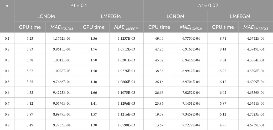
Table 4. Maximum error and CPU time obtained for Example 4 when $RE=5$.

Figure 5

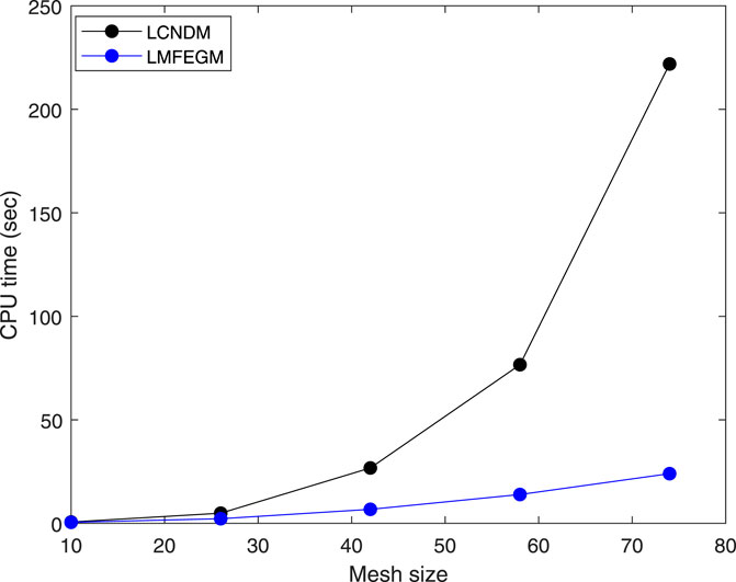
Figure 5. Comparison of CPU times of the LCNDM and LMFEGM for Example 4 with $T=1$, $N=100$, $\alpha =0.5$, and $RE=5$.

Example 5. We consider the time-fractional Burgers model (Equation 2) whose exact solution is given by

$w\left(\mathbf{x},t\right)=t{e}^{-{\left(x-0.5\right)}^2-{\left(y-0.5\right)}^2}.$

For this example, we apply the proposed methods to solve the time-fractional Burgers equation using $h=1/98$, $RE=100$, and the three final times $T=1.0$, $T=1.5$, and $T=2.0$. The corresponding results are tabulated in Table 5, from which we observe that the numerical solutions of the methods are close to the exact solution for different values of $T$. The computational times of the LCNDM are greater than those of the LMFEGM, which indicates the efficiency of the latter. Figure 6 displays the three-dimensional error profile when $T=2$, $h=1/98$, $N=50$, $\alpha =0.5$, and $RE=100$, which shows the accuracy of the proposed methods. All numerical simulations demonstrate the viability of the proposed methods and stress the computational superiority of the LMFEGM over the LCNDM in solving the time-fractional Burgers model.

Table 5

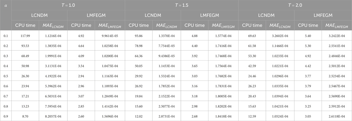
Table 5. Maximum error and CPU time obtained for Example 5 with $RE=100$ and $h=1/98$.

Figure 6

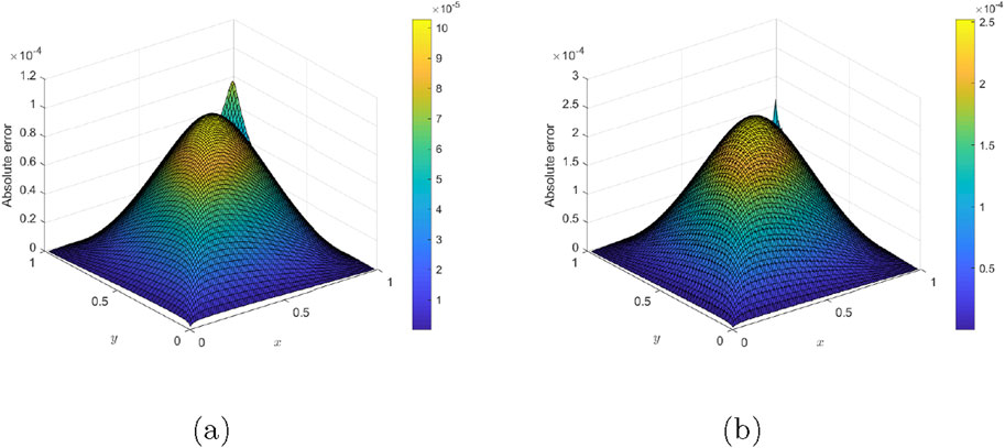
Figure 6. Three-dimensional error profile of Example 5 when $T=2$, $h=1/98$, $N=50$, $\alpha =0.5$, and $RE=100$. (a) LCNDM. (b) LMFEGM.

7 Conclusion

In this article, the LMFEGM is proposed for solving the two-dimensional time-fractional Burgers equation. The method employs the $L_1$ discretization formula for the fractional temporal derivative and a linearized difference scheme on a coarse mesh for the spatial derivatives. The LCNDM is also developed for comparison purposes. The stability and convergence of both methods are rigorously studied and proven via Fourier analysis. Five numerical simulations are carried out, and the obtained data are represented in Tables 1–5 along with Figures 2–6. Numerical results demonstrate that the LMFEGM is accurate and a good CPU time reducer; hence, it is computationally superior to the LCNDM in dealing with the time-fractional Burgers model. This is particularly useful when simulating complex physical problems governed by multi-dimensional, nonlinear, and nonlocal fractional models. In this regard, the LMFEGM can be extended for handling other high-dimensional fractional Burgers-type models [51] in the future. The combination of the LMFEGM with two-gird methods [52, 53, 53] is also a potential subject of further research. Finally, the extension of the proposed method to deal with fractional models that exhibit weak singularity at the initial time is another interesting avenue for future research.

Data availability statement

The original contributions presented in the study are included in the article/supplementary material; further inquiries can be directed to the corresponding author.

Author contributions

FS: Writing – original draft, Writing – review and editing.

Funding

The author(s) declare that financial support was received for the research and/or publication of this article. The author acknowledges the funding support provided by the Deanship of Research at the King Fahd University of Petroleum and Minerals (KFUPM), Kingdom of Saudi Arabia.

Acknowledgments

The author would like to thank the reviewers for their insightful comments that helped improve the article.

Conflict of interest

The authors declare that the research was conducted in the absence of any commercial or financial relationships that could be construed as a potential conflict of interest.

Generative AI statement

The author(s) declare that no Generative AI was used in the creation of this manuscript.

Publisher’s note

All claims expressed in this article are solely those of the authors and do not necessarily represent those of their affiliated organizations, or those of the publisher, the editors and the reviewers. Any product that may be evaluated in this article, or claim that may be made by its manufacturer, is not guaranteed or endorsed by the publisher.

References

1. Sales Teodoro G, Machado JT, De Oliveira EC. A review of definitions of fractional derivatives and other operators. J Comput Phys (2019) 388:195–208. doi:10.1016/j.jcp.2019.03.008

CrossRef Full Text | Google Scholar

2. Luchko Y. Fractional derivatives and the fundamental theorem of fractional calculus. Fractional Calculus Appl Anal (2020) 23(4):939–966. doi:10.1515/fca-2020-0049

CrossRef Full Text | Google Scholar

3. Vasily ET. Handbook of fractional calculus with applications, volume 5. Berlin: de Gruyter (2019).

Google Scholar

4. Partohaghighi M, Akgül A. Fractional study of the covid-19 model with different types of transmissions. Kuwait J Sci (2023) 50:153–162. doi:10.1016/j.kjs.2023.02.021

PubMed Abstract | CrossRef Full Text | Google Scholar

5. Liu S, Sun H, Yu H, Miao J, Cao Z, Zhang X. A framework for battery temperature estimation based on fractional electro-thermal coupling model. J Energ Storage (2023) 2063:107042. doi:10.1016/j.est.2023.107042

CrossRef Full Text | Google Scholar

6. Ionescu C, Lopes A, Copot D, Machado JT, Bates JHT. The role of fractional calculus in modeling biological phenomena: a review. Commun Nonlinear Sci Numer Simulation (2017) 51:141–159. doi:10.1016/j.cnsns.2017.04.001

CrossRef Full Text | Google Scholar

7. Zhang Y, Sun HG, Stowell HH, Zayernouri M, Hansen SE. A review of applications of fractional calculus in earth system dynamics. Chaos, Solitons and Fractals (2017) 102:29–46. doi:10.1016/j.chaos.2017.03.051

CrossRef Full Text | Google Scholar

8. Sun HG, Zhang Y, Baleanu D, Chen W, Chen YQ. A new collection of real world applications of fractional calculus in science and engineering. Commun Nonlinear Sci Numer Simulation (2018) 64:213–231. doi:10.1016/j.cnsns.2018.04.019

CrossRef Full Text | Google Scholar

9. Vasily ET. Mathematical economics: application of fractional calculus (2020).

Google Scholar

10. Priyendhu KS, Prakash P, Lakshmanan M. Invariant subspace method to the initial and boundary value problem of the higher dimensional nonlinear time-fractional pdes. Commun Nonlinear Sci Numer Simulation (2023) 122:107245. doi:10.1016/j.cnsns.2023.107245

CrossRef Full Text | Google Scholar

11. Song L, Zhang H. Application of homotopy analysis method to fractional kdv–burgers–kuramoto equation. Phys Lett A (2007) 367(1-2):88–94. doi:10.1016/j.physleta.2007.02.083

CrossRef Full Text | Google Scholar

12. Mustafa I. The approximate and exact solutions of the space-and time-fractional burgers equations with initial conditions by variational iteration method. J Math Anal Appl (2008) 345(1):476–484. doi:10.1016/j.jmaa.2008.04.007

CrossRef Full Text | Google Scholar

13. Saad KM, Al-Sharif EHF. Analytical study for time and time-space fractional burgers’ equation. Adv Difference Equations (2017) 2017(1):1–15. doi:10.1186/s13662-017-1358-0

CrossRef Full Text | Google Scholar

14. Alam Khan N, Ara A, Mahmood A. Numerical solutions of time-fractional burgers equations: a comparison between generalized differential transformation technique and homotopy perturbation method. Int J Numer Methods Heat and Fluid Flow (2012) 22(2):175–193. doi:10.1108/09615531211199818

CrossRef Full Text | Google Scholar

15. Mohebbi A. Analysis of a numerical method for the solution of time fractional burgers equation. Bull Iranian Math Soc (2018) 44:457–480. doi:10.1007/s41980-018-0031-z

CrossRef Full Text | Google Scholar

16. Vong S, Lyu P. Unconditional convergence in maximum-norm of a second-order linearized scheme for a time-fractional burgers-type equation. J Scientific Comput (2018) 76:1252–1273. doi:10.1007/s10915-018-0659-0

CrossRef Full Text | Google Scholar

17. Duangpan A, Boonklurb R, Treeyaprasert T. Finite integration method with shifted Chebyshev polynomials for solving time-fractional burgers’ equations. Mathematics (2019) 7(12):1201. doi:10.3390/math7121201

CrossRef Full Text | Google Scholar

18. Qiu W, Chen H, Zheng X. An implicit difference scheme and algorithm implementation for the one-dimensional time-fractional burgers equations. Mathematics Comput Simulation (2019) 166:298–314. doi:10.1016/j.matcom.2019.05.017

CrossRef Full Text | Google Scholar

19. Li L, Li D. Exact solutions and numerical study of time fractional burgers’ equations. Appl Maths Lett (2020) 100:106011. doi:10.1016/j.aml.2019.106011

CrossRef Full Text | Google Scholar

20. Onal M, Esen A. A crank-nicolson approximation for the time fractional burgers equation. Appl Maths Nonlinear Sci (2020) 5(2):177–184. doi:10.2478/amns.2020.2.00023

CrossRef Full Text | Google Scholar

21. Yaseen M, Abbas M. An efficient computational technique based on cubic trigonometric b-splines for time fractional burgers’ equation. Int J Comput Maths (2020) 97(3):725–738. doi:10.1080/00207160.2019.1612053

CrossRef Full Text | Google Scholar

22. Sweilam NH, Al-Mekhlafi SM, Baleanu D. Nonstandard finite difference method for solving complex-order fractional burgers’ equations. J Adv Res (2020) 25:19–29. doi:10.1016/j.jare.2020.04.007

PubMed Abstract | CrossRef Full Text | Google Scholar

23. Yadav S, Pandey RK. Numerical approximation of fractional burgers equation with atangana–baleanu derivative in caputo sense. Chaos, Solitons and Fractals (2020) 133:109630. doi:10.1016/j.chaos.2020.109630

CrossRef Full Text | Google Scholar

24. Akram T, Abbas M, Riaz MB, Ismail AI, Ali NM. An efficient numerical technique for solving time fractional burgers equation. Alexandria Eng J (2020) 59(4):2201–2220. doi:10.1016/j.aej.2020.01.048

CrossRef Full Text | Google Scholar

25. Huang Y, Mohammadi Zadeh F, Skandari MHN, Tehrani HA, Tohidi E. Space–time Chebyshev spectral collocation method for nonlinear time-fractional burgers equations based on efficient basis functions. Math Methods Appl Sci (2021) 44(5):4117–4136. doi:10.1002/mma.7015

CrossRef Full Text | Google Scholar

26. Vieru D, Fetecau C, Ali Shah N, Chung JD. Numerical approaches of the generalized time-fractional burgers’ equation with time-variable coefficients. J Funct Spaces (2021) 2021:1–14. doi:10.1155/2021/8803182

CrossRef Full Text | Google Scholar

27. Abdi N, Aminikhah H, Refahi Sheikhani AH, Alavi J, Taghipour M. An efficient explicit decoupled group method for solving two–dimensional fractional burgers’ equation and its convergence analysis. Adv Math Phys (2021) 2021:1–20. doi:10.1155/2021/6669287

CrossRef Full Text | Google Scholar

28. Li H, Wu Y. Artificial boundary conditions for nonlinear time fractional burgers’ equation on unbounded domains. Appl Maths Lett (2021) 120:107277. doi:10.1016/j.aml.2021.107277

CrossRef Full Text | Google Scholar

29. Sadiq Hashmi M, Wajiha M, Yao S-W, Ghaffar A, Mustafa I. Cubic spline based differential quadrature method: a numerical approach for fractional burger equation. Results Phys (2021) 26:104415. doi:10.1016/j.rinp.2021.104415

CrossRef Full Text | Google Scholar

30. Zhang Y, Feng M. A local projection stabilization virtual element method for the time-fractional burgers equation with high Reynolds numbers. Appl Maths Comput (2023) 436:127509. doi:10.1016/j.amc.2022.127509

CrossRef Full Text | Google Scholar

31. Wang Y, Sun T. Two linear finite difference schemes based on exponential basis for two-dimensional time fractional burgers equation. Physica D: Nonlinear Phenomena (2024) 459:134024. doi:10.1016/j.physd.2023.134024

CrossRef Full Text | Google Scholar

32. Maji S, Srinivasan N. Error analysis for discontinuous galerkin method for time-fractional burgers’ equation. Math Methods Appl Sci (2024) 47(12):9703–9717. doi:10.1002/mma.10089

CrossRef Full Text | Google Scholar

33. Xing Z, Sun W, Zhu X. A fast l1 formula on tanh meshes for time fractional burgers equations. Int J Geometric Methods Mod Phys (2024). doi:10.1142/s0219887824400413

CrossRef Full Text | Google Scholar

34. Diethelm K, Kiryakova V, Luchko Y, Machado JAT, Tarasov VE. Trends, directions for further research, and some open problems of fractional calculus. Nonlinear Dyn (2022) 107(4):3245–3270. doi:10.1007/s11071-021-07158-9

CrossRef Full Text | Google Scholar

35. Salama FM, Hamid NNA, Ali NHM, Ali U. An efficient modified hybrid explicit group iterative method for the time-fractional diffusion equation in two space dimensions. AIMS Maths (2022) 7(2):2370–2392. doi:10.3934/math.2022134

CrossRef Full Text | Google Scholar

36. Salama FM, Hamid NNA, Ali U, Ali NHM. Fast hybrid explicit group methods for solving 2d fractional advection-diffusion equation. AIMS Maths (2022) 7(9):15854–15880. doi:10.3934/math.2022868

CrossRef Full Text | Google Scholar

37. Salama FM, Balasim AT, Ali U, Khan MA. Efficient numerical simulations based on an explicit group approach for the time fractional advection–diffusion reaction equation. Comput Appl Maths (2023) 42(4):157. doi:10.1007/s40314-023-02278-x

CrossRef Full Text | Google Scholar

38. Salama FM, Fairag F. On numerical solution of two-dimensional variable-order fractional diffusion equation arising in transport phenomena. AIMS Math (2024) 9(1):340–370. doi:10.3934/math.2024020

CrossRef Full Text | Google Scholar

39. Salama FM, Norhashidah H, Hamid NNA. Efficient hybrid group iterative methods in the solution of two-dimensional time fractional cable equation. Adv Difference Equations (2020) 2020(1):1–20. doi:10.1186/s13662-020-02717-7

CrossRef Full Text | Google Scholar

40. Asim Khan M, Ali NHM, Hamid NNA. The design of new high-order group iterative method in the solution of two-dimensional fractional cable equation. Alexandria Eng J (2021) 60(4):3553–3563. doi:10.1016/j.aej.2021.01.008

CrossRef Full Text | Google Scholar

41. Fouad MS. On numerical simulations of variable-order fractional cable equation arising in neuronal dynamics. Fractal and Fractional (2024) 8(5):282. doi:10.3390/fractalfract8050282

CrossRef Full Text | Google Scholar

42. Salama FM, Ali U, Ali A. Numerical solution of two-dimensional time fractional mobile/immobile equation using explicit group methods. Int J Appl Comput Maths (2022) 8(4):188. doi:10.1007/s40819-022-01408-z

PubMed Abstract | CrossRef Full Text | Google Scholar

43. Salama FM, Fairag F. A numerical algorithm with parallel implementation for variable-order fractional mobile/immobile equation. J Appl Maths Comput (2025) 71(2):2433–2471. doi:10.1007/s12190-024-02321-y

CrossRef Full Text | Google Scholar

44. Abdi N, Aminikhah H, Sheikhani AHR. High-order rotated grid point iterative method for solving 2d time fractional telegraph equation and its convergence analysis. Comput Appl Maths (2021) 40:54–26. doi:10.1007/s40314-021-01451-4

CrossRef Full Text | Google Scholar

45. Ali A, Abdeljawad T, Iqbal A, Akram T, Abbas M. On unconditionally stable new modified fractional group iterative scheme for the solution of 2d time-fractional telegraph model. Symmetry (2021) 13(11):2078. doi:10.3390/sym13112078

CrossRef Full Text | Google Scholar

46. Bonkile MP, Awasthi A, Lakshmi C, Mukundan V, Aswin VS. A systematic literature review of burgers’ equation with recent advances. Pramana (2018) 90:69–21. doi:10.1007/s12043-018-1559-4

CrossRef Full Text | Google Scholar

47. Bastian ER. Microfluidics: modeling, mechanics and mathematics. Amsterdam: Elsevier (2017).

Google Scholar

48. Peng X, Xu D, Qiu W. Pointwise error estimates of compact difference scheme for mixed-type time-fractional burgers’ equation. Maths Comput Simulation (2023) 208:702–726. doi:10.1016/j.matcom.2023.02.004

CrossRef Full Text | Google Scholar

49. Kong D, Xu Y, Zheng Z. A hybrid numerical method for the kdv equation by finite difference and sinc collocation method. Appl Maths Comput (2019) 355:61–72. doi:10.1016/j.amc.2019.02.031

CrossRef Full Text | Google Scholar

50. Karatay I, Kale N, Bayramoglu S. A new difference scheme for time fractional heat equations based on the crank-nicholson method. Fractional Calculus Appl Anal (2013) 16(4):892–910. doi:10.2478/s13540-013-0055-2

CrossRef Full Text | Google Scholar

51. Peng X, Qiu W, Hendy AS, Zaky MA. Temporal second-order fast finite difference/compact difference schemes for time-fractional generalized burgers’ equations. J Scientific Comput (2024) 99(2):52. doi:10.1007/s10915-024-02514-4

CrossRef Full Text | Google Scholar

52. Peng X, Qiu W, Wang J, Ma L. A novel temporal two-grid compact finite difference scheme for the viscous burgers’ equation. Adv In Appl Maths Mech (2024) 16(6):1358–1380. doi:10.4208/aamm.oa-2022-0302

CrossRef Full Text | Google Scholar

53. Chen H, Qiu W, Zaky MA, Ahmed SH. A two-grid temporal second-order scheme for the two-dimensional nonlinear volterra integro-differential equation with weakly singular kernel. Calcolo (2023) 60(1):13. doi:10.1007/s10092-023-00508-6

CrossRef Full Text | Google Scholar