Reduced-order aerodynamic model of a starting plate with discrete-vortex merging

This study employs potential flow theory with a discrete-vortex method to model the unsteady aerodynamics of a flat plate, with a particular focus on the coupled dynamics of leading-edge and trailing-edge vortices (LEVs and TEVs). Through the simulation of an impulsively starting plate at 45$°$ angle-of-attack, we demonstrate that the initial strong lift production maintaining for approximately two chord lengths of travel arises from differential vortex advection rates—rapid TEV shedding generates strong positive lift, while slow LEV movement over the plate produces weaker negative contributions. This finding provides new physical insight into the LEV-induced lift enhancement that it is likely a consequence of reduced negative lift rather than enhanced positive lift generation, as the LEV slows down to become more stable. To reduce computational complexity while preserving physical fidelity, we develop a novel vortex merge algorithm based on conservations of circulation and momentum, coupled with a condition enforcing minimal velocity perturbation to the plate surface. Through comparisons with both single-vortex and full discrete-vortex models, we demonstrate the superior performance of our reduced-order approach in capturing wake structure evolution and predicting unsteady lift, while balancing computational efficiency across a tunable range of precision. The developed model proves especially effective for long-time or small-time-step calculations, offering significant computational savings without compromising the fidelity of vortex dynamics or force predictions.

1 Introduction

Research in low-Reynolds-number unsteady aerodynamics has been profoundly influenced by studies of insect flight and flapping wings, motivated by the remarkable lift-generating capabilities observed in these biological systems [1–5]. Early experimental investigations employing flow visualization techniques [6–8] revealed that lift enhancement is fundamentally linked to unsteady wing motion, which promotes the formation and maintenance of a stable leading-edge vortex (LEV). Such an LEV exhibits significantly greater stability than its steady-flow counterpart, resulting in delayed vortex shedding and stall [9–13].

The theoretical explanation of lift enhancement via vortex attachment traces back to Saffman & Sheffield [14], who employed two-dimensional (2D) potential flow theory to demonstrate that a steady flow over a wing with an attached vortex produces increased lift. Subsequent developments by Chow & Huang [15] and Mourtos & Brooks [16] extended this framework to account for airfoil thickness, camber, and spanwise flow effects. These early studies have established that vortex stabilization on the upper airfoil surface provides enhanced lift, based on the assumption that the vortex remains stabilized at an equilibrium position for Kutta–Joukowski lift calculations. The stabilization mechanism of the LEV was first investigated by Rossow [17], who introduced a point sink at the vortex core to model the effects of spanwise flow on vorticity transport. This formulation enabled quasi-steady modeling of vortex dynamics through a linear system framework, permitting evaluation of vortex equilibrium and stability characteristics; however, the analysis ultimately failed to demonstrate LEV stabilization. Most recently, Xia & Mohseni [18] resolved this issue by replacing the point sink with a finite-area sink, allowing fully coupled vortex-sink interactions. This modification enabled the first mathematical proof of LEV stabilization under conditions of spanwise vorticity transport. However, the quasi-steady formulation inherently neglects the unsteady characteristics of flapping wings, including the dynamic vortex formation and shedding processes.

Subsequent modeling efforts have focused on resolving the unsteady dynamics of flapping wings through vortex methods to better capture wake evolution and lift generation mechanisms. Significant improvements in unsteady aerodynamic modeling have been achieved through high-fidelity resolution of wake vorticity distributions, implemented via two primary approaches, the discrete-vortex methods [19–26] and the continuous vortex sheet/panel techniques [27–30]. In particular, Ansari et al.s model [22, 31] showed good agreement in both force predictions and wake development in comparison with previous experimental results [1, 32]. Recent advances in these frameworks have yielded accurate predictions of both wake vortex dynamics and unsteady aerodynamic forces, particularly through the development of theoretical formulations for rotating flat plates [23] and arbitrary airfoil geometries [26, 33] as well as fundamental criteria for vortex shedding, including the leading-edge suction parameter [24] and generalized unsteady Kutta conditions [26, 34–36].

The continuous introduction of new vortex elements into the wake leads to progressively increasing computational costs. Alternatively, the complexity of the wake system can be significantly reduced by modeling only the main vortex cores with individual point vortices. Specifically, attached vortices with varying circulations are evolved based on the Brown–Michael equation [37], which essentially requires the vortex force to be conserved for a growing vortex. And detached vortices are treated as freely-advected vortices with frozen circulations. For example, Michelin & Smith [38] applied this approach to modeling vortex shedding dynamics of multi-edge bodies, while Wang & Eldredge [39] developed a two-vortex model for coupled LEV–TEV dynamics, incorporating an impulse-matching scheme to eliminate nonphysical force jumps during vortex shedding. However, the single-vortex models are over-simplified in resolving near-field vortical structures of complicate geometries, leading to inaccuracies in both vortex evolution and force predictions. A more fundamental limitation is the absence of physical criteria for vortex shedding timing, which constrains the models’ ability to capture long-term wake development. Recently, Darakananda & Eldredge [40] and Dumoulin et al. [33] developed a hybrid low-order vortex method that combines near-field vortex sheet resolution with far-field representation by a limited number of detached point vortices, where the transition between these representations is governed by a threshold condition based on vortex force discrepancy. However, this approach remains imperfect from a physical perspective, as the detachment of point vortices does not fully align with the natural timing of coherent vortex formation and shedding in the wake.

This work is focused on further exploring model reduction based on our previous unsteady aerodynamic model of a flat plate [23]. Our reduction approach here was inspired by Spalart [41] and Ansari et al. [22] who implemented vortex merge/amalgamation schemes based on minimizing velocity variation at the far field away from the merging site. However, in addition to their merging principle, we propose that the merge process should also conserve the total momentum of all vortices involved so as to prevent spurious force generation. Through comparisons with experiment, single-vortex models, and the original discrete-vortex model, we aim to demonstrate the computational efficiency and accuracy of the present model for possible low-order applications.

2 Theoretical approach

To investigate unsteady aerodynamics of a 2D flat plate, the present study employs the unsteady potential flow model developed by Xia & Mohseni [23], with discrete vortices introduced to capture the shear layer dynamics and vortex shedding behaviors at both the leading and trailing edges, as illustrated in Figure 1. This framework entails the default assumption of inviscid, incompressible 2D flow, which has several limitations. For example, it is unable to capture three-dimensional effects, such as vortex breakdown and tip vortex that are essential to a low-aspect-ratio wing. Furthermore, the viscous effects cannot be sufficiently resolved. Although vortex formation and shedding can be predicted using unsteady Kutta condition, major uncertainties could arise due to its inability to account for the formation of boundary layer and the viscous diffusion of shear layer and vortex core. Nevertheless, in terms of reduced-order modeling, potential flow still has its own advantage. In particular, it gives explicit expression of the flow field without solving the Navier–Stokes equation, thereby providing a mathematical foundation for analyzing the vortex dynamics while maintaining computational tractability. Combined with the discrete-vortex method, it is able to offer reasonably accurate predictions of the wake vortex evolutions and aerodynamic forces, especially the lift resulting from vortex circulation.

Figure 1

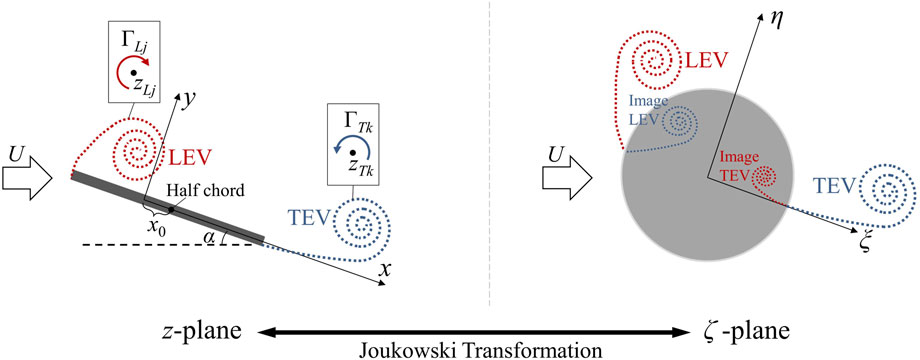
Figure 1. Diagram illustrating the unsteady potential flow model of a 2D flat plate, with discrete vortices shedding from the leading and trailing edges. The flow in the physical $z$-plane is mapped to that in the virtual $\zeta$-plane using Joukowski transformation.

2.1 Unsteady potential flow model

We start by introducing the unsteady potential flow model in Figure 1, where the flow around a flat plate in the laboratory coordinate system (denoted as the $z$-plane, $z=x+iy$) is mapped to an equivalent flow around a cylinder in an imaginary $\zeta$-plane $(\zeta =\xi +i\eta )$ via the Joukowski transformation,

$z=\zeta +\frac{a^2}{\zeta }+x_0,(1)$

where $a$ denotes the cylinder radius, related to the chord length $c$ of the flat plate by $a=c/4$. In Equation 1, $x_0$ represents the offset distance between the plate’s midpoint and the origin. The incoming flow has a time-varying velocity, $U(t)$, and a fixed angle of attack (AoA), $\alpha$.

Considering the background flow and the vortex singularities in Figure 1, we may apply the rule of superposition and the circle theorem [42] to express the complex potential in $\zeta$-plane as

$\begin{array}{cc}\hfill w_{\zeta }\left(\zeta \right)& =\underset{\text{Translational}}{\underbrace{|U|e^{-i\alpha }\left(\zeta +x_0\right)+|U|e^{i\alpha }\left(a^2/\zeta +x_0\right)}}\hfill \\ \hfill & -\frac{i}{2\pi }{\displaystyle \underset{\text{LEVs}}{{\displaystyle \underbrace{{\displaystyle \sum _{j=1}^M}{\mathrm{\Gamma }}_{Lj}\ln \left(\frac{\zeta -{\zeta }_{Lj}}{\zeta -a^2/{\bar{\zeta }}_{Lj}}\right)}}}}-\frac{i}{2\pi }{\displaystyle \underset{\text{TEVs}}{{\displaystyle \underbrace{{\displaystyle \sum _{k=1}^N}{\mathrm{\Gamma }}_{Tk}\ln \left(\frac{\zeta -{\zeta }_{Tk}}{\zeta -a^2/{\bar{\zeta }}_{Tk}}\right)}}}},\hfill \end{array}(2)$

where the first two terms account for the translational motion of the plate, while the last two terms describe the induced effects of the discrete vortices associated with the LEVs and TEVs, including those from their image vortices within the cylinder. Here, $M$ and $N$ denote the total number of vortices in the LEVs and TEVs, respectively. $L_j$ and $T_k$ refer to the $j$th and $k$th vortices in the LEVs and TEVs, respectively; they correspond to the locations $z_{Lj}$ and $z_{Tk}$ in the physical plane and ${\zeta }_{Lj}$ and ${\zeta }_{Tk}$ in the cyliner plane, with the circulations of ${\mathrm{\Gamma }}_{Lj}$ and ${\mathrm{\Gamma }}_{Tk}$.

The evaluation of Equation 2 requires precise determination of both circulations and positions for all discrete point vortices. For the circulation, each vortex element generating from either the leading or trailing edge is assigned a strength governed by the classical steady-state Kutta condition:

$\frac{\partial w_{\zeta }\left(\zeta \right)}{\partial \zeta }=0\text{for}\zeta \to \pm a.(3)$

This condition enforces stagnation points at the edges of the cylinder in the $\zeta$-plane, which corresponds to maintaining finite velocities at the sharp edges of the flat plate in the physical $z$-plane. While this condition is inherently satisfied at the trailing edge, its validity at the leading edge is restricted to large AoA, which is justified by the presence of significant reverse flow on the windward side [23]. Consequently, the current analysis focuses only on the large-AoA scenario where this assumption holds. In the present discrete-vortex framework, Equation 3 can be further calculated as

$\frac{\partial w_{\zeta }^{*}\left(\zeta \right)}{\partial \zeta }-\frac{i{\mathrm{\Gamma }}_{Lm}}{2\pi }\frac{\partial }{\partial \zeta }\left(\ln \left(\frac{\zeta -{\zeta }_{Lm}}{\zeta -a^2/{\bar{\zeta }}_{Lm}}\right)\right)-\frac{i{\mathrm{\Gamma }}_{Tn}}{2\pi }\frac{\partial }{\partial \zeta }\left(\ln \left(\frac{\zeta -{\zeta }_{Tn}}{\zeta -a^2/{\bar{\zeta }}_{Tn}}\right)\right)=0\text{for}\zeta \to \pm a,(4)$

where $L_m$ and $T_n$ are the new vortices forming at the leading and trailing edges, respectively. $w_{\zeta }^{*}(\zeta )$ represents the complex potential excluding the contributions from the newly generated vortices. The unknowns in Equation 4 are the positions, ${\zeta }_{Lm}$ and ${\zeta }_{Tn}$, and circulations, ${\mathrm{\Gamma }}_{Lm}$ and ${\mathrm{\Gamma }}_{Tn}$, of the two new vortices. To close the system, we adopt a key physical assumption that the vorticity flux from the edge to the shear layer is treated as quasi-steady, with its rate determined by the local flow advection. It follows that the initial placement of new vortices satisfies the 1/3-arc rule [22, 23, 43], meaning that each new vortex should be positioned at the one-third point of the arc between the shedding edge and the previously released vortex. Of course, this arc has to be tangential to the sharp edge according to the Kutta condition. Then, the vortex positions $z_{Lm}$ and $z_{Tn}$ obtained through this geometric condition can be transformed back to the $\zeta$-plane and substituted into Equation 4 to solve for the unknown circulations, ${\mathrm{\Gamma }}_{Lm}$ and ${\mathrm{\Gamma }}_{Tn}$.

Once generated, the vortices in the wake are assumed to hold constant circulations, as dictated by the Helmholtz’s laws of vortex motion. However, the spatial evolution of a vortex follows Lagrangian advection via a de-singularized velocity (for a point vortex $L_v$ in the LEVs):

$\begin{array}{cc}{u}_{Lv}-i{v}_{Lv}=\hfill & \hfill \frac{{\zeta }_{Lv}^2}{2\pi \left({\zeta }_{Lv}^2-a^2\right)}\left[2\pi |U|\left(e^{-i\alpha }-\frac{a^2{e}^{i\alpha }}{{\zeta }_{Lv}^2}\right)-{\displaystyle \sum _{j=1,j\ne v}^M}\frac{i{\mathrm{\Gamma }}_{Lj}}{{\zeta }_{Lv}-{\zeta }_{Lj}}\right.\\ \hfill & \hfill \left.+,{\displaystyle \sum _{j=1}^M},\frac{i{\mathrm{\Gamma }}_{Lj}}{{\zeta }_{Lv}-a^2/{\bar{\zeta }}_{Lj}},-{\displaystyle \sum _{k=1}^N}\left(\frac{i{\mathrm{\Gamma }}_{Tk}}{{\zeta }_{Lv}-{\zeta }_{Tk}}-\frac{i{\mathrm{\Gamma }}_{Tk}}{{\zeta }_{Lv}-a^2/{\bar{\zeta }}_{Tk}}\right)\right]\\ \hfill & \hfill +\frac{i{\mathrm{\Gamma }}_{Lv}}{\pi }\frac{{\zeta }_{Lv}{a}^2}{{\left(a^2-{\zeta }_{Lv}^2\right)}^2}.\end{array}(5)$

The final term of Equation 5 represents the Routh correction [44, 45], accounting for the self-induced velocity due to the vortex’s interaction with its image vortex in the cylinder. An analogous expression for a vortex $T_v$ in the TEVs can be obtained through substitution of indices and excluding the singularity at $\zeta ={\zeta }_{Tv}$.

Based on the potential flow model, the unsteady aerodynamic force can be calculated by employing the unsteady Bernoulli equation and then computing the unsteady Blasius integrals [23], which gives

$\begin{array}{cc}\hfill F_x-i{F}_y& =\underset{\text{Added}\text{Mass}}{\underbrace{2\pi \rho a^2|\dot{U}|\left(e^{-i\alpha }-e^{i\alpha }\right)}}\hfill \\ \hfill & -i\rho {\displaystyle \sum _{j=1}^M}\underset{\text{LEVs}}{\underbrace{\left[{\mathrm{\Gamma }}_{Lj}\frac{d}{dt}\left({\bar{\zeta }}_{Lj}-\frac{a^2}{{\zeta }_{Lj}}\right)\right]}}-i\rho {\displaystyle \sum _{k=1}^N}\underset{\text{TEVs}}{\underbrace{\left[{\mathrm{\Gamma }}_{Tk}\frac{d}{dt}\left({\bar{\zeta }}_{Tk}-\frac{a^2}{{\zeta }_{Tk}}\right)\right]}},\hfill \end{array}(6)$

where $\rho$ is fluid density. This formula suggests that a major unsteady force contribution, other than the ‘added mass’ effect owing to background flow acceleration, is from the LEVs and TEVs in the wake. Specifically, these terms highlight the importance of the relative advective movements between the vortices and their image counterparts.

2.2 Vortex merge algorithm

In the potential flow model, the incorporation of the discrete-vortex method enables the tracking of wake vortex evolution and the estimation of unsteady aerodynamic forces arising from vortex motion. However, as vortices are continuously introduced into the flow field at each time step, the computational cost escalates and the efficiency degrades significantly over time or with reduced time steps owing to the accumulating vortex population. A critical question thus arises: can a vortex merge algorithm be devised to amalgamate proximate vortices, thereby improving computational efficiency without compromising much simulation fidelity? To address this, we focus on the most basic scenario of a double-vortex system and propose two physical hypotheses governing the merging process:

(i) The merging process must obey the basic conservations of circulation and momentum.

(ii) The global flow field should remain largely unaffected by the merging.

Based on the preceding analysis, the merging process of two point vortices with circulations ${\mathrm{\Gamma }}_1$ and ${\mathrm{\Gamma }}_2$ is illustrated in Figure 2. The resultant vortex after merging has a circulation ${\mathrm{\Gamma }}_3$, which satisfies ${\mathrm{\Gamma }}_3={\mathrm{\Gamma }}_1+{\mathrm{\Gamma }}_2$ by the conservation of circulation. The momentum equation for a single vortex (with circulation vector $\mathbf{\Gamma }$) can be expressed in terms of a vortex force, ${\mathbf{f}}_v$, as [46].

${\mathbf{f}}_v+\rho \left(\mathbf{U}-{\mathbf{U}}_v\right)\times \mathbf{\Gamma }=0,(7)$

where $\mathbf{U}$ denotes the background flow velocity, which is also the vortex velocity as if it were a free vortex, and ${\mathbf{U}}_v$ is the actual advective velocity of the vortex. Equation 7 dictates that any net force acting on a vortex, resulting from its interaction with the surrounding fluid or structures, must be balanced by a deviation in its advective velocity from that of an equivalent free vortex. Based on the vortex locations before and after merging, as shown in Figure 2, Equation 7 can be respectively derived for the merging vortices in the forms of

${\mathbf{f}}_{v1}+\rho \left[\frac{{\mathbf{P}}_1^{\prime }\left(t+\mathrm{\Delta }t\right)-{\mathbf{P}}_1\left(t\right)}{\mathrm{\Delta }t}-\frac{{\mathbf{P}}_3\left(t+\mathrm{\Delta }t\right)-{\mathbf{P}}_1\left(t\right)}{\mathrm{\Delta }t}\right]\times {\mathbf{\Gamma }}_1=0(8)$

${\mathbf{f}}_{v2}+\rho \left[\frac{{\mathbf{P}}_2^{\prime }\left(t+\mathrm{\Delta }t\right)-{\mathbf{P}}_2\left(t\right)}{\mathrm{\Delta }t}-\frac{{\mathbf{P}}_3\left(t+\mathrm{\Delta }t\right)-{\mathbf{P}}_2\left(t\right)}{\mathrm{\Delta }t}\right]\times {\mathbf{\Gamma }}_2=0,(9)$

where ${\mathbf{P}}_1(t)$ and ${\mathbf{P}}_2(t)$ denote the initial positions of the vortices, and ${\mathbf{P}}_3(t+\mathrm{\Delta })$ is the position of the merged vortex location after an infinitesimal merging period $\mathrm{\Delta }t$. Here, ${\mathbf{P}}_1^{\prime }(t+\mathrm{\Delta }t)$ and ${\mathbf{P}}_2^{\prime }(t+\mathrm{\Delta }t)$ correspond to the hypothetical positions of the merging vortices as if they were advected freely without merging. Within the present potential flow framework, the summation of Equations 8, 9 yields

$\frac{\left(f_{v1}+f_{v2}\right)\mathrm{\Delta }t}{\rho }=\left(z_1^{\prime }-z_3\right){\mathrm{\Gamma }}_1+\left(z_2^{\prime }-z_3\right){\mathrm{\Gamma }}_2,(10)$

where $z_1^{\prime }$, $z_2^{\prime }$, and $z_3$ are the complex-plane positions at $t+\mathrm{\Delta }t$, corresponding to ${\mathbf{P}}_1^{\prime }$, ${\mathbf{P}}_2^{\prime }$, and ${\mathbf{P}}_3$, respectively. Now, hypothesis (i) can be implemented by requiring the momentum conservation $(f_{v1}+f_{v2})$ and the circulation conservation $({\mathrm{\Gamma }}_3={\mathrm{\Gamma }}_1+{\mathrm{\Gamma }}_2)$, which reduces Equation 10 to

$z_3=\frac{{\mathrm{\Gamma }}_1{z}_1^{\prime }+{\mathrm{\Gamma }}_2{z}_2^{\prime }}{{\mathrm{\Gamma }}_3}.(11)$

This result reveals that the merged vortex’s position $z_3$ is determined by the circulation-weighted centroid of the double-vortex system—a direct consequence of momentum conservation. Equation 11 aligns with the findings of Spalart [41], derived via Taylor expansion to match the far-field induced velocities pre- and post-merging. Mathematically, Equation 11 applies to the merging of any vortex pair, irrespective of their rotation directions. Physically, however, merging is only meaningful for same-signed vortices, meaning ${\mathrm{\Gamma }}_1$, ${\mathrm{\Gamma }}_2$, and ${\mathrm{\Gamma }}_3$ all have the sign. This is because, in the actual viscous flow, two approaching same-signed vortices are subject to vorticity diffusion that tends to smear their individual vorticity peaks into a single peak, resulting in the vortex merge. Conversely, opposite-sign vortices undergo annihilation as vorticity diffusion enforces a zero-vorticity boundary between them, thereby preventing the merge. It should be noted that, vortex annihilation remains a challenge for the present singularity-based model, which cannot yield the information of vorticity distribution that dictates the diffusive process of annihilation. Nevertheless, future effort can be made to offer an approximate solution to this problem, based on modeling the characteristic annihilation time of two approaching vortices.

Figure 2

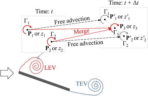
Figure 2. Merging process of two point vortices. Initially, the two vortices (of circulations ${\mathrm{\Gamma }}_1$ and ${\mathrm{\Gamma }}_2$) are located at ${\mathbf{P}}_1$ and ${\mathbf{P}}_2$, respectively. After a period of $\mathrm{\Delta }t$, they merge into one vortex of circulation ${\mathrm{\Gamma }}_3$ at ${\mathbf{P}}_3$.

Regarding hypothesis (ii), while the change in velocity induction inevitably introduces some near-field disturbances—making complete neutrality impossible—this hypothesis can be relaxed to a problem-specific condition. In this study, as aerodynamic forces are of primary interest, which result from the interactions between the plate and the wake vortices as indicated from Equation 6), this condition can be established based on minimizing the change in velocity induction exerted by the vortex system on the plate surface. To establish such a condition, we consider the induced velocity at $z_s$, a point on the plate surface that is closest to the merged point $z_3$. The velocity difference between the cases with and without merging can be expressed as

$\begin{array}{c}\hfill \mathrm{\Delta }{V}_s=-\frac{i}{2\pi }\left(\frac{{\mathrm{\Gamma }}_1}{z_s-z_1^{\prime }}+\frac{{\mathrm{\Gamma }}_2}{z_s-z_2^{\prime }}-\frac{{\mathrm{\Gamma }}_3}{z_s-z_3}\right).\end{array}(12)$

By further applying the Taylor expansion to the first two terms at $z_1^{\prime }=z_3$ and $z_2^{\prime }=z_3$, respectively, Equation 12 can be further derived as

$\begin{array}{cc}\hfill 2\pi i\mathrm{\Delta }{V}_s& =\frac{{\mathrm{\Gamma }}_1}{z_s-z_3}\left[1+\frac{z_1^{\prime }-z_3}{z_s-z_3}+{\left(\frac{z_1^{\prime }-z_3}{z_s-z_3}\right)}^2+o\left({\left(\frac{z_1^{\prime }-z_3}{z_s-z_3}\right)}^2\right)\right]\hfill \\ \hfill & +\frac{{\mathrm{\Gamma }}_2}{z_s-z_3}\left[1+\frac{z_2^{\prime }-z_3}{z_s-z_3}+{\left(\frac{z_2^{\prime }-z_3}{z_s-z_3}\right)}^2+o\left({\left(\frac{z_2^{\prime }-z_3}{z_s-z_3}\right)}^2\right)\right]-\frac{{\mathrm{\Gamma }}_3}{z_s-z_3},\hfill \end{array}(13)$

where the convergence of the Taylor series requires $|z_1^{\prime }-z_3|<|z_s-z_3|$ and $|z_2^{\prime }-z_3|<|z_s-z_3|$.

Combining Equations 11, 13 and neglecting the small-order terms yield

$\begin{array}{cc}\hfill \left|2\pi i\mathrm{\Delta }{V}_s\right|& \approx \left|\frac{{\mathrm{\Gamma }}_1}{z_s-z_3}{\left(\frac{z_1^{\prime }-z_3}{z_s-z_3}\right)}^2+\frac{{\mathrm{\Gamma }}_2}{z_s-z_3}{\left(\frac{z_2^{\prime }-z_3}{z_s-z_3}\right)}^2\right|\hfill \\ \hfill & \le \left|\frac{{\mathrm{\Gamma }}_1}{z_s-z_3}\right|\left|{\left(\frac{z_1^{\prime }-z_3}{z_s-z_3}\right)}^2\right|+\left|\frac{{\mathrm{\Gamma }}_2}{z_s-z_3}\right|\left|{\left(\frac{z_2^{\prime }-z_3}{z_s-z_3}\right)}^2\right|.\hfill \end{array}(14)$

Equation 14 can be recast to give the inequality of the relative change in induced velocity at $z_s$:

$\begin{array}{c}\hfill \left|\frac{\mathrm{\Delta }{V}_s}{V_s}\right|\le {\delta }_M=\frac{{\mathrm{\Gamma }}_1}{{\mathrm{\Gamma }}_3}\left|{\left(\frac{z_1^{\prime }-z_3}{z_s-z_3}\right)}^2\right|+\frac{{\mathrm{\Gamma }}_2}{{\mathrm{\Gamma }}_3}\left|{\left(\frac{z_2^{\prime }-z_3}{z_s-z_3}\right)}^2\right|,\end{array}(15)$

where $V_s$ is the velocity induced by the merged vortex (of circulation ${\mathrm{\Gamma }}_3$) at $z_s$. To satisfy hypothesis (ii), which requires the velocity induced by the merging vortices on the plate surface being negligible, the parameter ${\delta }_M$ must take an infinitesimal value. Consequently, we can prescribe ${\delta }_M$ as a small threshold value, serving as the criterion for determining whether two vortices should undergo instantaneous merging.

3 Results and discussion

The unsteady potential flow framework with discrete vortices has been demonstrated to yield accurate predictions of both wake evolutions and unsteady lift variations in the previous work [23]. The present study extends this analysis by examining two key aspects: (1) the physical mechanisms underlying different contributions to unsteady lift generation on an impulsively starting plate, and (2) the efficacy of the proposed vortex merge algorithm for model reduction.

3.1 Contributions to unsteady lift generation

The lift generation mechanisms are investigated through simulating an impulsively starting flat plate experiment, originally conducted by Dickinson and Gotz [32]. The flat plate has a chord length of 5 cm with an angle of attack fixed at 45$°$. The plate accelerates uniformly at 62.5 cm/s² from rest, attaining a steady-state velocity of 10 cm/s after 0.16 s. The plate motion ceases after a travel distance $(s)$ of 7.5 chord lengths. The characteristic Reynolds number (Re) is estimated to be 192 based on the chord length and the steady-state plate speed. Figure 3A (to row) displays the flow visualization images from the original experimental study [32], showing four representative snapshots at travel distances ranging from 1 to 4 chord lengths. The second row plots the corresponding flow field predictions obtained from the current model. A time step of 0.005 s was employed in the simulations, which has been demonstrated to provide an optimal balance between computational accuracy and efficiency [23].

Figure 3

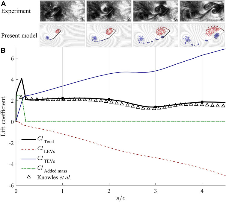
Figure 3. (A) Flow visualization images (top) of a starting plate at $45°$ AoA during 1–4 chord lengths of travel [32]. Snapshots of streamline and wake pattern (bottom) simulated by the present model. (B) The corresponding lift coefficient variation with chord length of travel $(s/c)$. Here, the lift coefficient $(Cl)$ is estimated as $Cl=2L/(\rho U^{2}c)$, with the lift given by $L=F_y\cos \alpha -F_x\sin \alpha$. The total lift $C{l}_{\text{Total}}$ is validated against Knowles et al.s CFD result [47]. Based on Equation 6, contributions to $C{l}_{\text{Total}}$ can be divided into three components originating from the LEVs $(C{l}_{\text{LEVs}})$, TEVs $(C{l}_{\text{TEVs}})$, and added mass $(C{l}_{\text{Added\hspace{0.17em}mass}})$, respectively. It is interesting to note that LEVs generate negative lift while TEVs generate positive lift.

Next, the predicted lift coefficient is compared with validated CFD results (Re = 250) from Knowles et al. [47] in Figure 3B, showing overall good agreement. For more validation cases, the interested readers are referred to our previous works that have demonstrated the performance of this discrete vortex model in predicting the wake structures and aerodynamic/hydrodynamic forces of not only the staring or the pitching plates [23] but also NACA-series airfoils with various prescribed swimming motions [26]. Here, the lift coefficient is computed using Equation 6 based on the total force component of $F_x+i{F}_y$ normal to the incoming flow. Combining Figures 3A,B, substantial lift generation occurs during the initial 2 chord lengths of travel, coinciding with leading-edge vortex (LEV) formation and trailing-edge vortex (TEV) shedding. Specifically, analysis of the lift contribution components reveals that the post-startup peak results from the combined effects of the added-mass and the positive lift contributed by the TEV. However, Knowles et al.s CFD result exhibits a much weaker initial peak, indicating a lower added-mass contribution associated with the initial acceleration. This discrepancy likely originates from the viscous effect in the CFD simulation, which forms a boundary layer that moves with the plate, thereby reducing the effective acceleration experienced by the plate. This indicates that the present inviscid model has a tendency of overestimating aerodynamic force during rapid flow transition. During steady plate motion, the TEV and LEV exhibit opposing trends—the former maintains gradual increase of positive lift while the latter shows progressive decrease of negative lift. This behavior suggests that the net positive lift stems from the differential between TEV and LEV contributions established during the initial phase of plate startup, which is maintained up to $s=2c$. However, after that, there appears a pronounced lift reduction, i.e., stall, corresponding to a plateaued lift generation associated with the TEV; physically, this is likely attributed to the formation of the secondary TEV, which disrupts the feeding shear layer of the primary TEV, as is evident from Figure 3A. When $s>3c$, the lift generation from TEVs resumes increasing, leading to the total lift recovery.

It should be emphasized that this result provides important physical insights into vortex-dominated unsteady lift generation mechanisms, which has intrinsic connections to insect flight. While previous experimental observations have reported the prominent correlation between significant lift enhancement and a stabilized LEV, our analysis reveals that this phenomenon should not be attributed to the LEV alone. In fact, the apparent LEV ‘stabilization’ likely reflects its slower advective velocity relative to the TEV. Our findings from Figure 3 suggest that the positive net lift arises from a balance between vortex contributions—the faster shedding TEV provides substantial positive lift while the LEV with a slower downstream advection generates comparatively weaker negative lift. From a vortex dynamics perspective, the characteristic stall behavior occurs when the feeding shear layer of the primary TEV ruptures, thereby inhibiting the shear layer’s downstream advection and further reducing positive lift generation from the newly formed TEV. Detailed flow analysis reveals that this transition stems from LEV–TEV interactions. As evident in Figure 3, the growing LEV extends to the trailing edge after $s=2c$, which significantly influences the trailing-edge flow field. This interaction exerts strong impact on the Kutta condition at the trailing edge, which further disturbs the feeding shear layer of the existing TEV. Consequently, the detachment of the previous TEV and the subsequent formation of a new TEV are promoted, causing an interruption to the total lift generation.

Despite the overall promising performance demonstrated through this simple case, the present discrete-vortex model has an inherent limitation in handling viscous diffusion, which is associated with the growth of shear layer thickness or the spreading of vortex core. Specifically, viscosity can influence the redistribution of vorticity inside the LEV, thereby rendering the model inaccurate in capturing the vortex core location, which could further affect force predictions. Furthermore, viscosity also plays an important role in the vortex-surface interaction. As the LEV or TEV approaches the plate surface, the vortex circulation would decay owing to vorticity annihilation between the vortex and its induced shear layer along the surface, which is of opposite-sign vorticity; similar effect is also prominent in the interaction of an LEV–TEV couple. Without resolving such effects, the potential flow model likely over-predicts the vortex circulation, which could affect not only the magnitude of the force calculation but also the timings for vortex roll-up and shedding, causing uncertainties in predicting the long-term evolutions.

3.2 Reduced-order model performance

The growing complexity of discrete-vortex systems in long-duration or small-time-step simulations necessitates model simplification. This study explores the vortex amalgamation scheme, based on applying the merging criterion established in Section 3 to systematically reduce the discrete vortex population while preserving the main vortex dynamics. The performance of this approach is quantified by comparing the variations of lift coefficient, flow field pattern, and the vortex population with alternative reduced-order models.

Before presenting the simulation results obtained based on discrete-vortex merging, we first examine the performance of single-vortex models to offer references for both wake capture and lift estimation of the starting-plate problem. The analysis here serves two purposes. One is to assess whether the over-simplified single-vortex representations can adequately capture the flow field and vortex dynamics; the other is to provide context for evaluating the newly proposed amalgamation approach. Here, four different models are implemented, including a baseline model named the ‘discrete-vortex’, which refers to the original discrete-vortex model without any reduction, and three single-vortex models, namely, ‘single-LEV’, ‘single-TEV’, and ‘single-LEV&TEV’. For the single-vortex representations, each model employs a single point vortex of constant circulation to account for either the primary LEV, the primary TEV, or both. It should be mentioned that, in previous single-vortex models [38, 39], the vortex circulation was treated as a time-dependent variable, with its location evolved based on the Brown–Michael equation [37]. However, our implementation here has two key distinctions. First, we introduce one more point vortex near the shedding edges, in addition to the main vortex, to represent the effect of the feeding shear layer. Furthermore, new vortices are continuously introduced at each time step to model the vorticity feeding of the shear layer, meanwhile the preceding vortex in the feeding shear layer is merged into the main vortex; the position of the merged LEV is determined by Equation 11 that was derived based on the momentum conservation. In this way, our approach is consistent with the essence of the Brown–Michael equation while offering greater authority in capturing the dynamics of the feeding shear layer, which has crucial influences on the vorticity generation and vortex shedding conditions at the edges.

To implement the single-vortex models, all cases are initialized with the ‘discrete-vortex’ setting during the first chord length of travel. At $s=c$, the single-vortex algorithms are activated by first merging all the discrete vortices in either the LEV or TEV based on the conservations of circulation and momentum, which can be readily extended from hypothesis (i) in Section 2.2. This transition scheme ensures smooth switching between vortex representations while matching the fundamental physics. Then, at each subsequent time step, a new vortex is introduced near the edge to capture the physics of vorticity generation, whereas the preceding vortex merges with the main vortex to emulate vorticity feeding from the edge-attached shear layer.

The simulated flow fields and wake patterns are presented in Figure 4, which enables quantitative evaluation of the single-vortex methods through direct comparison with the ‘discrete-vortex’ model (benchmark) at representative flow evolution stages. The ‘single-LEV’ demonstrates qualitative agreement with the ‘discrete-vortex’ results up to $s=3c$. However, by $s=4c$, discernible differences emerge in the TEV topology during the formation of the secondary TEV, revealing the limitations of the ‘single-LEV’ model in resolving near-field flow features. Notably, these discrepancies appear confined to the near field, as the far-field wake characteristics, particularly the primary TEV, remain consistent between Figures 4A,B. The single-TEV model exhibits significant shortcomings in capturing both the TEV position and LEV configuration, as shown in Figure 4C. This deficiency stems primarily from the model’s inability to properly account for secondary TEV generation—a critical process evident in the ‘discrete-vortex’ solution after $s=2c$, where the extensively-grown LEV disturbs the trailing-edge shear layer and triggers the formation of a secondary TEV. However, in the ‘single-TEV’ scenario, all vorticity generated from the trailing edge is absorbed into the primary TEV, creating an artificially strong TEV that induces the unphysical down-wash of the LEV off the trailing edge (final snapshot of Figure 4C). As seen in Figure 4D, the combined ‘single-LEV&TEV’ model inherits limitations from both constituent approaches, resulting in similarly compromised performance in resolving the flow field pattern and vortex positions.

Figure 4

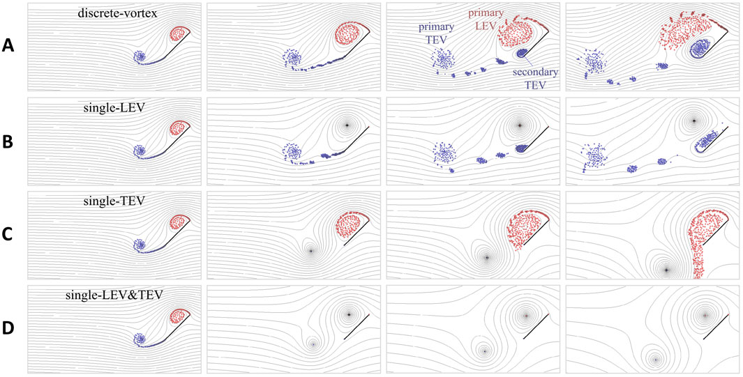
Figure 4. Snapshots of simulated flow field at 1–4 chord lengths of travel. The result of (A) the ‘discrete-vortex’ model serves as a benchmark, which is compared with those of three single-vortex models: (B) ‘single-LEV’, (C) ‘single-TEV’, and (D) ‘single-LEV&TEV’.

Figure 5A further compares the lift calculations corresponding to the simulated results in Figure 4. For a more comprehensive assessment of the different models, the total circulations of both the LEV and TEV as well as the horizontal positions $s_v$ of their centroids (circulation-weighted) are tracked in Figures 5B,C. In general, the results reveal inferior performance of the single-vortex models in tracking the unsteady lift variation compared to the ‘discrete-vortex’ model. A particularly notable discrepancy emerges at the one-chord-length point of merging transition, where both the ‘single-LEV’ and ‘single-LEV&TEV’ models display abrupt lift decline upon activation. This is somewhat surprising as the merging process conserves the total momentum of all merged vortices, meaning that the aerodynamic force should be maintained in theory. The apparent contradiction can be explained again from the perspective of vortex–edge interactions. Upon vortex merging, while the momentum conservation holds for isolated vortex system, the rate of vorticity generation at the plate edge varies dramatically owing to the change in the induced velocity by the different vorticity distribution. This is particularly evident from the abrupt increase in the LEV circulation magnitude after $s/c=1$, for the ‘single-LEV’ and ‘single-LEV&TEV’ models shown in Figure 5B. Consequently, the sudden lift drop can be attributed to the abruptly-intensified LEV circulation, given that LEV advection yields negative lift as discussed in Section 3.1. This lift drop implies a limitation of the single-vortex model that, even when satisfying the Brown–Michael equation, it cannot adequately resolve the dynamical effects of discrete vortex clouds, especially when the vortex is in the near field. Interestingly, the ‘single-TEV’ model demonstrates a smoother post-merging transition in unsteady lift and the rate of circulation generation at trailing edge seems to be less affected by the merging event at $s/c=1$. This can be understood that the TEV is farther away from its vorticity-generating edge, so the induced velocity at the edge by the TEV is less affected by the change in its vorticity distribution. Although the ‘single-TEV’ exhibits better merging initialization, significant deviations develop with increasing travel distance due to the model’s fundamental inability to accurately represent near-field vortical structures, as discussed previously.

Figure 5

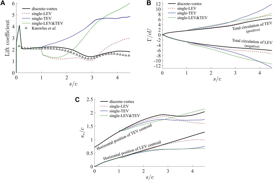
Figure 5. Comparisons of (A) unsteady lift coefficient, (B) vortex circulation, and (C) horizontal locations of vortex centroid predicted by the ‘discrete-vortex’ model with the single-vortex models, corresponding to the different cases in Figure 4. Knowles et al.s CFD result [47] is plotted as a reference in (A).

Based on the data in Figure 5, the performance of the three single-vortex models are further assessed quantitatively in Table 1 via computing the mean absolute errors (MAEs) of five variables, including the lift coefficient $C_l$, the nondimensional total circulations ${\mathrm{\Gamma }}_{\mathit{LEV}}/cU$ and ${\mathrm{\Gamma }}_{\mathit{TEV}}/cU$ of the LEV and TEV, and the horizontal positions $s_{\mathit{LEV}}$ and $s_{\mathit{TEV}}$ of the LEV and TEV’s centroids. Note that these MAEs are calculated relative to the benchmark results of the ‘discrete-vortex’ model, based on the data in the range of $1<s/c<4.5$. Among these three models, the ‘single-LEV’ corresponds to the lowest errors in tracking the lift coefficient and wake vortices, consistent with the observations from Figures 4, 5. The results of the single-vortex models offer two general implications for future improvement. The first is to enhance the representation of near-field vorticial structures, especially the vorticity-feeding shear layer. On the other hand, a proper physical condition is needed to precisely determine the transition timing for the shedding of the old vortex and the generation of the new vortex. Given the inherent limitations of the single-vortex approach in the near-field representation, it makes the discrete-vortex approach indispensable for problems requiring accurate wake and force predictions, despite its greater computational expense.

Table 1

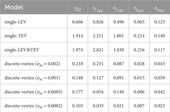
Table 1. Mean absolute errors (MAE) of $Cl$, $\mathrm{\Gamma }$, and $s_v$ for different reduced-order models.

Next, we investigate the performance of the vortex merging scheme based on the discrete-vortex framework. The parameter ${\delta }_M$, which is the merging criterion (Equation 15) controlling the error of the vortex system’s induced velocity on the plate surface, is varied between 0.0002 and 0.002. The simulation results are presented in Figure 6, showing that the reduced-order models are able to capture the overall flow field characteristics, including the position and morphology of the primary vortices as well as the formation of the secondary TEV, even at larger ${\delta }_M$ values; and the fidelity of the wake details tends to improve as ${\delta }_M$ decreases. Figure 7 further shows good agreement of the predictions by different simplified models with the original ‘discrete-vortex’ model, through the comparisons of the lift calculations as well as the evolutions of vortex circulation and location, demonstrating improved accuracy with smaller ${\delta }_M$ values in general. Similar to the analysis of the single-vortex models, the MAEs corresponding to the data in Figure 7 are also evaluated for the different merging models, as listed in Table 1. The error values are significantly lower than those of the single-vortex models. Furthermore, the MAEs also exhibit general declining trends as the merging threshold parameter ${\delta }_M$ decreases, quantitatively justifying the efficacy of ${\delta }_M$ in tuning the accuracy of the discrete-vortex models.

Figure 6

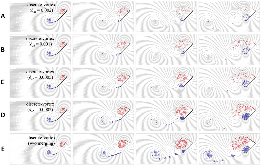
Figure 6. Snapshots of simulated flow field at 1–4 chord lengths of travel. The ‘discrete-vortex’ results with different vortex-merge levels (A–D) are compared with (E) the benchmark case without merging. For the cases employing the proposed merge scheme, the merging criterion ${\delta }_M$ is configured as (A) 0.002, (B) 0.001, (C) 0.0005, and (D) 0.0002, respectively.

Figure 7

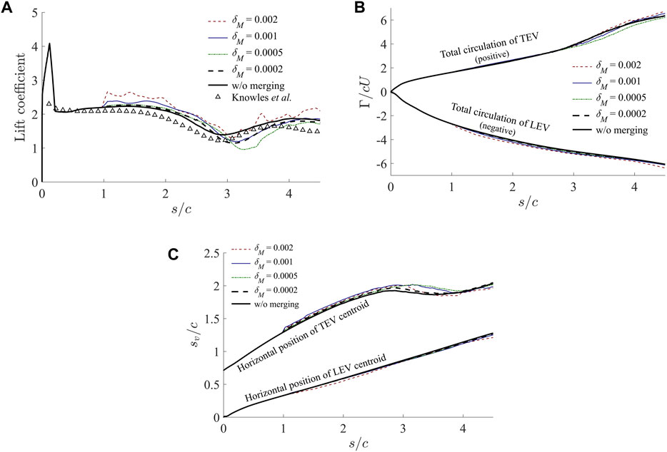
Figure 7. Comparisons of (A) unsteady lift coefficient, (B) vortex circulation, and (C) horizontal locations of vortex centroid predicted by the ‘discrete-vortex’ model with various settings for vortex merging, corresponding to the different cases in Figure 6. Knowles et al.s CFD result [47] is plotted as a reference in (A).

Last, to assess effectiveness of the vortex merge algorithm in reducing the system’s complexity, the evolutions of the discrete vortex population are compared in Figure 8, with $M$ and $N$ being the total numbers of discrete vortices associated with LEV and TEV, respectively. It reveals that larger ${\delta }_M$ values lead to greater reduction, particularly for the primary TEV that quickly advects downstream, which is also evident from Figure 6. Furthermore, the results also demonstrate that the present model-reduction scheme tends to promote far-field reduction while maintaining near-field resolution, which exactly aligns with our original motivation. Owing to this feature of preferential reduction in the far field, it is likely that the vortex population would achieve approximate saturation as time proceeds. This presents a significant computational advantage over conventional discrete-vortex models, especially for long-term or small-time-step simulations, as it inhibits the linear growth of vortex population while preserving essential flow physics in the critical near-field wake. The overall good performance in both computational accuracy and efficiency justifies our proposal for the reduced-order aerodynamic model based on discrete-vortex merging.

Figure 8

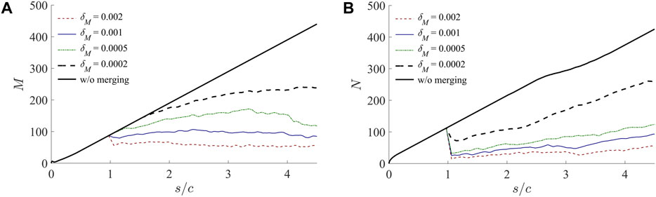
Figure 8. Comparison of vortex population among ‘discrete-vortex’ models of different vortex-merge levels gauged by ${\delta }_M$. (A) Vortex population $M$ in LEV, (B) vortex population $N$ in TEV.

Before closing, it is worth discussing the practical choice of ${\delta }_M$. Based on Table 1, we can divide the ${ϵ}_{Cl}$ by the average $C_l$ of the benchmark model during $1<s/c<4.5$. This yields the relative MAEs to be 12.1%, 8.2%, 9.8%, and 5.7% for the four different levels of ${\delta }_M$, respectively. For applications involving low-order aerodynamic force prediction, it is usually desirable to keep the error within 10%, corresponding to ${\delta }_M\le 0.001$. As for the efficiency, based on the data in Figure 8, we can divide the total vortex population, $M+N$, by that of the benchmark model to obtain the relative vortex population. Consequently, the mean relative vortex populations during $1<s/c<4.5$ are estimated to be 19.5%, 30.7%, 43.5%, and 67.2% for the four merging levels, respectively. Assuming a requirement of at least 50% reduction in computational cost, we should select ${\delta }_M\ge 0.0005$. In balancing the above conditions for accuracy and efficiency, we recommend setting ${\delta }_M$ between 0.0005 and 0.001. This guideline may be applicable to more complicated flow situations, as the present merge scheme is derived to consider a general vortex–body interaction.

4 Conclusion

This study employs the potential flow theory to examine the aerodynamics of a flat plate undergoing unsteady translational motion at an angle-of-attack of 45$°$. A discrete-vortex approach is adopted to capture the coupled dynamics of the LEVs and TEVs in the wake. The LEV and TEV contributions to lift generation are first investigated by modeling the problem of an impulsively starting flat plate. The results reveal that, during the initial phase, downstream advection of the LEV generates negative lift, while the TEV produces a stronger positive lift owing to its significantly faster streamwise advection. This differential advection behavior creates a net positive lift that persists for approximately two chord lengths of travel, when the LEV undergoes substantial growth with relatively slow advection. This offers new insight into the experimental observation of lift enhancement by LEV stabilization that the slowed-down advection of the LEV causes less negative lift rather than more positive lift, from an unsteady aerodynamics perspective. A dynamic stall occurs beyond two chord lengths as the extensive-grown LEV interacts with the trailing-edge flow, leading to disruption of the TEV feeding shear layer and triggering formation of a new TEV. Unlike its predecessor, this secondary TEV tends to linger over the plate under the LEV influence, resulting in diminished positive lift production and the observed stall behavior.

To improve computational efficiency while preserving physical fidelity, a vortex merge scheme is developed based on two physical assumptions for the merging process: (i) conservations of circulation and momentum and (ii) negligible velocity difference induced on the plate surface. The latter ensures a sufficient accuracy in resolving vortex-plate interactions, especially in the critical near-plate region where vortex-induced effects dominate. The efficacy of the proposed reduced-order model is evaluated in comparison with the single-vortex models as well as the original discrete-vortex model without reduction. The analysis of the single-vortex models serves as a reference to demonstrate their limitations in accurately resolving the near-field wake, when a distributed vorticity field is replaced by a single vortex. In contrast, the vortex merge algorithm developed in this study exhibits substantially improved performance, which is able to accurately capturing both flow field evolution and lift generation while maintaining computational efficiency; the balance between computation precision and cost can be adjusted through a threshold merge parameter ${\delta }_M$. The results show promises for long-term or small-time-step simulations, where significant computational saving is possible without compromising physical fidelity. Finally, to offer a practical guideline for selecting ${\delta }_M$, we recommend its range to be 0.0005-0.001 in satisfying the conditions of $<$10% error in lift prediction and $>$50% reduction in computational cost.

Data availability statement

The raw data supporting the conclusions of this article will be made available by the authors, without undue reservation.

Author contributions

XX: Conceptualization, Investigation, Writing – review and editing, Formal Analysis, Writing – original draft. LS: Writing – review and editing, Formal Analysis, Visualization.

Funding

The author(s) declare that financial support was received for the research and/or publication of this article. The authors gratefully acknowledge the financial support from the National Natural Science Foundation of China (nos. 12072194, 22227901, and 52006139).

Acknowledgments

The authors would like to acknowledge the valuable insights and comments offered by Prof. Kamran Mohseni.

Conflict of interest

The authors declare that the research was conducted in the absence of any commercial or financial relationships that could be construed as a potential conflict of interest.

Generative AI statement

The author(s) declare that no Generative AI was used in the creation of this manuscript.

Any alternative text (alt text) provided alongside figures in this article has been generated by Frontiers with the support of artificial intelligence and reasonable efforts have been made to ensure accuracy, including review by the authors wherever possible. If you identify any issues, please contact us.

Publisher’s note

All claims expressed in this article are solely those of the authors and do not necessarily represent those of their affiliated organizations, or those of the publisher, the editors and the reviewers. Any product that may be evaluated in this article, or claim that may be made by its manufacturer, is not guaranteed or endorsed by the publisher.

References

1. Dickinson MH, Lehmann FO, Sane SP. Wing rotation and the aerodynamic basis of insect flight. Science (1999) 284:1954–60. doi:10.1126/science.284.5422.1954PubMed Abstract | CrossRef Full Text | Google Scholar

2. Shyy W, Lian Y, Tang J, Viieru D, Liu H. Aerodynamics of low Reynolds number flyers. New York, NY (2008). doi:10.1017/CBO9780511551154CrossRef Full Text | Google Scholar

3. Liu G, Dong H, Li C. Vortex dynamics and new lift enhancement mechanism of wing–body interaction in insect forward flight. J Fluid Mech (2016) 795:634–51. doi:10.1017/jfm.2016.175CrossRef Full Text | Google Scholar

4. Bomphrey R, Nakata T, Phillips N, Walker S. Smart wing rotation and trailing-edge vortices enable high frequency mosquito. Nature (2017) 544:92–5. doi:10.1038/nature21727PubMed Abstract | CrossRef Full Text | Google Scholar

5. Oh S, Lee B, Park H, Choi H, Kim ST. A numerical and theoretical study of the aerodynamic performance of a hovering rhinoceros beetle (Trypoxylus dichotomus). J Fluid Mech (2020) 885:A18. doi:10.1017/jfm.2019.962CrossRef Full Text | Google Scholar

6. Ellington C, van der Berg C, Willmott A, Thomas A. Leading-edge vortices in insect flight. Nature (1996) 384:626–30. doi:10.1038/384626a0CrossRef Full Text | Google Scholar

7. van den Berg C, Ellington CP. The three-dimensional leading-edge vortex of a ‘hovering’ model hawkmoth. Phil Trans R Soc Lond B (1997) 352:329–40. doi:10.1098/rstb.1997.0024CrossRef Full Text | Google Scholar

8. Willmott AP, Ellington CP, Thomas ALR. Flow visualization and unsteady aerodynamics in the flight of the hawkmoth Manduca sexta. Phil Trans R Soc Lond B (1997) 352:303–16. doi:10.1098/rstb.1997.0022CrossRef Full Text | Google Scholar

9. Maxworthy T. The fluid dynamics of insect flight. Ann Rev Fluid Mech (1981) 13:329–50. doi:10.1146/annurev.fl.13.010181.001553CrossRef Full Text | Google Scholar

10. Ellington CP. The aerodynamics of hovering insect flight. IV. Aerodynamic mechanisms. Phil Trans R Soc Lond B (1984) 305:79–113. doi:10.1098/rstb.1984.0052CrossRef Full Text | Google Scholar

11. Birch JM, Dickinson MH. Spanwise flow and the attachment of the leading-edge vortex on insect wings. Nature (2001) 412:729–33. doi:10.1038/35089071PubMed Abstract | CrossRef Full Text | Google Scholar

12. DeVoria AC, Mohseni K. On the mechanism of high-incidence lift generation for steadily translating low-aspect-ratio wings. J Fluid Mech (2017) 813:110–26. doi:10.1017/jfm.2016.849CrossRef Full Text | Google Scholar

13. Linehan T, Mohseni K. On the maintenance of an attached leading-edge vortex via model bird alula. J Fluid Mech (2020) 897:A17. doi:10.1017/jfm.2020.364CrossRef Full Text | Google Scholar

14. Saffman PG, Sheffield JS. Flow over a wing with an attached free vortex. Stud Appl Math (1977) 57:107–17. doi:10.1002/sapm1977572107CrossRef Full Text | Google Scholar

15. Huang MK, Chow CY. Trapping of a free vortex by Joukowski airfoils. AIAA J (1982) 20:292–8. doi:10.2514/3.7913CrossRef Full Text | Google Scholar

16. Mourtos NJ, Brooks M. Flow past a flat plate with a vortex/sink combination. J Appl Mech (1996) 63:543–50. doi:10.1115/1.2788902CrossRef Full Text | Google Scholar

17. Rossow V. Lift enhancement by an externally trapped vortex. J Aircr (1978) 15:618–25. doi:10.2514/3.58416CrossRef Full Text | Google Scholar

18. Xia X, Mohseni K. A theory on leading-edge vortex stabilization by spanwise flow. J Fluid Mech (2023) 970:R1. doi:10.1017/jfm.2023.613CrossRef Full Text | Google Scholar

19. Katz J. A discrete vortex method for the non-steady separated flow over an airfoil. J Fluid Mech (1981) 102:315–28. doi:10.1017/S0022112081002668CrossRef Full Text | Google Scholar

20. Streitlien K, Triantafyllou MS. Force and moment on a joukowski profile in the presence of point vortices. AIAA J (1995) 33:603–10. doi:10.2514/3.12621CrossRef Full Text | Google Scholar

21. Yu Y, Tong B, Ma H. An analytic approach to theoretical modeling of highly unsteady viscous flow excited by wing flapping in small insects. Acta Mech Sin (2003) 19:508–16. doi:10.1007/BF02484543CrossRef Full Text | Google Scholar

22. Ansari SA, Zbikowski R, Knowles K. Non-linear unsteady aerodynamic model for insect-like flapping wings in the hover. part 2: implementation and validation. Proc Inst Mech Eng G (2006) 220:169–86. doi:10.1243/09544100JAERO50CrossRef Full Text | Google Scholar

23. Xia X, Mohseni K. Lift evaluation of a two-dimensional pitching flat plate. Phys Fluids (2013) 25:091901. doi:10.1063/1.4819878CrossRef Full Text | Google Scholar

24. Ramesh K, Gopalarathnam A, Granlund K, Ol MV, Edwards JR. Discrete-vortex method with novel shedding criterion for unsteady aerofoil flows with intermittent leading-edge vortex shedding. J Fluid Mech (2014) 751:500–38. doi:10.1017/jfm.2014.297CrossRef Full Text | Google Scholar

25. Li J, Wu Z. Unsteady lift for the Wagner problem in the presence of additional leading/trailing edge vortices. J Fluid Mech (2015) 769:182–217. doi:10.1017/jfm.2015.118CrossRef Full Text | Google Scholar

26. Xia X, Mohseni K. Unsteady aerodynamics and vortex-sheet formation of a two-dimensional airfoil. J Fluid Mech (2017) 830:439–78. doi:10.1017/jfm.2017.513CrossRef Full Text | Google Scholar

27. Jones MA. The separated flow of an inviscid fluid around a moving flat plate. J Fluid Mech (2003) 496:405–41. doi:10.1017/S0022112003006645CrossRef Full Text | Google Scholar

28. Pullin DI, Wang ZJ. Unsteady forces on an accelerating plate and application to hovering insect flight. J Fluid Mech (2004) 509:1–21. doi:10.1017/S0022112004008821CrossRef Full Text | Google Scholar

29. Shukla RK, Eldredge JD. An inviscid model for vortex shedding from a deforming body. Theor Comput Fluid Dyn (2007) 21:343–68. doi:10.1007/s00162-007-0053-2CrossRef Full Text | Google Scholar

30. DeVoria AC, Mohseni K. Vortex sheet roll-up revisited. J Fluid Mech (2018) 855:299–321. doi:10.1017/jfm.2018.663CrossRef Full Text | Google Scholar

31. Ansari SA, Zbikowski R, Knowles K. Non-linear unsteady aerodynamic model for insect-like flapping wings in the hover. part 1. methodology and analysis. Proc Inst Mech Eng G (2006) 220:61–83. doi:10.1243/09544100JAERO49CrossRef Full Text | Google Scholar

32. Dickinson MH, Gotz KG. Unsteady aerodynamic performance of model wings at low Reynolds numbers. J Exp Biol (1993) 174:45–64. doi:10.1242/jeb.174.1.45CrossRef Full Text | Google Scholar

33. Dumoulin D, Eldredge JD, Chatelain P. A lightweight vortex model for unsteady motion of airfoils. J Fluid Mech (2023) 977:A22. doi:10.1017/jfm.2023.997CrossRef Full Text | Google Scholar

34. DeVoria AC, Mohseni K. The vortex-entrainment sheet in an inviscid fluid: theory and separation at a sharp edge. J Fluid Mech (2019) 866:660–88. doi:10.1017/jfm.2019.134CrossRef Full Text | Google Scholar

35. Taha H, Rezaei AS. Viscous extension of potential-flow unsteady aerodynamics: the lift frequency response problem. J Fluid Mech (2019) 868:141–75. doi:10.1017/jfm.2019.159CrossRef Full Text | Google Scholar

36. Zhu W, McCrink MH, Bons JP, Gregory JW. The unsteady kutta condition on an airfoil in a surging flow. J Fluid Mech (2020) 893:R2. doi:10.1017/jfm.2020.254CrossRef Full Text | Google Scholar

37. Brown CE, Michael WH. Effect of leading-edge separation on the lift of a delta wing. J Astronaut Sci (1954) 21:690–4. doi:10.2514/8.3180CrossRef Full Text | Google Scholar

38. Michelin S, Smith SGL. An unsteady point vortex method for coupled fluid-solid problems. Theor Comput Fluid Dyn (2009) 23:127–53. doi:10.1007/s00162-009-0096-7CrossRef Full Text | Google Scholar

39. Wang C, Eldredge JD. Low-order phenomenological modeling of leading-edge vortex formation. Theor Comput Fluid Dyn (2013) 27:577–98. doi:10.1007/s00162-012-0279-5CrossRef Full Text | Google Scholar

40. Darakananda D, Eldredge JD. A versatile taxonomy of low-dimensional vortex models for unsteady aerodynamics. J Fluid Mech (2019) 858:917–48. doi:10.1017/jfm.2018.792CrossRef Full Text | Google Scholar

41. Spalart P. Direct numerical simulation of a turbulent boundary layer up to r_θ = 1410. J Fluid Mech (1988) 187:61–98. doi:10.1017/s0022112088000345CrossRef Full Text | Google Scholar

42. Milne-Thomson LM. Theoretical aerodynamics. Mineola, NY, USA: Dover (1958).

Google Scholar

43. Mason RJ. Fluid locomotion and trajectory planning for shape-changing robots. Pasadena, CA: California Institute of Technology (2002). Ph.D. thesis.

Google Scholar

44. Lin CC. On the motion of vortices in two dimensions-I. existence of the Kirchhoff-Routh function. Proc Natl Acad Sci (1941) 27:570–5. doi:10.1073/pnas.27.12.570PubMed Abstract | CrossRef Full Text | Google Scholar

45. Clements RR. An inviscid model of two-dimensional vortex shedding. J Fluid Mech (1973) 57:321–36. doi:10.1017/S0022112073001187CrossRef Full Text | Google Scholar

46. Saffman PG. Vortex dynamics. Cambridge, UK: Cambridge University Press (1992).

Google Scholar

47. Knowles K, Wilkins P, Ansari S, Zbikowski R. Integrated computational and experimental studies of flapping-wing micro air vehicle aerodynamics. In: Proceedings of the 3rd international symposium on integrating CFD and experiments in aerodynamics. CO, United States: U.S. Air Force Academy (2007). p. 1–15.

Google Scholar

Glossary

$\mathit{z}$ complex coordinate of the physical plane

$\mathit{x}$ horizontal coordinate of the physical plane

$\mathit{y}$ vertical coordinate of the physical plane

$\mathit{\zeta }$ complex coordinate of the imaginary plane

$\mathit{\xi }$ horizontal coordinate of the imaginary plane

$\mathit{\eta }$ vertical coordinate of the imaginary plane

$\mathit{a}$ cylinder radius of the imaginary plane

$\mathit{c}$ chord length of the flat plate

$\mathit{s}$ distance traveled by the plate

${\mathit{s}}_{\mathit{v}}$ horizontal location of a vortex centroid

${\mathit{x}}_{\mathbf{0}}$ offset distance of the coordinate origin

$\mathit{U}$ incoming flow velocity magnitude

$\mathit{\alpha }$ angle of attack

${\mathit{w}}_{\mathit{\zeta }}$ complex potential in the $\mathit{\zeta }$-plane

$\mathit{t}$ time

$\mathbf{\Delta }\mathit{t}$ time increment

$\mathit{M}$ total number of vortices in the LEVs

$\mathit{N}$ total number of vortices in the TEVs

$\mathbf{\Gamma }$ vortex circulation

$\mathit{u}$ $\mathit{x}$-component velocity

$\mathit{v}$ $\mathit{y}$-component velocity

${\mathit{F}}_{\mathit{x}}$ $\mathit{x}$-component aerodynamic force

${\mathit{F}}_{\mathit{y}}$ $\mathit{y}$-component aerodynamic force

$\mathit{\rho }$ density

${\mathbf{f}}_{\mathit{v}}$ vortex force

$\mathbf{U}$ background flow velocity

${\mathbf{U}}_{\mathit{v}}$ advective velocity of a vortex

$\mathbf{\Gamma }$ directional vortex circulation

$\mathbf{P}$ vortex position in Cartesian coordinate

$\mathit{V}$ complex velocity

$\mathrm{\Delta }\mathit{V}$ complex velocity difference

${\mathit{\delta }}_{\mathit{M}}$ threshold merge parameter

$\mathit{C}\mathit{l}$ coefficient of lift

$\mathit{L}$ lift (force magnitude)

$\mathit{ϵ}$ mean absolute error