Interfacial stability control of MHD Bingham fluids in micro-porous MEMS structures via fractal analysis

This study investigates Magnetohydrodynamics (MHD) interfacial stability in Bingham fluids moving in micro-porous MEMS structures with fractal space characteristics. The study uses nonlinear boundary conditions to study motion equations, resulting in a nonlinear partial differential equation for interface displacement with complex coefficients. The study also uses a modified Lindstedt-Poincaré transformation to express the elevation amplitude equation in fractal space, which is converted to a linear form using the harmonic equivalent linearization approach (HELA). The study presents diagrams to illustrate and interpret the resulting stability characteristics, providing valuable insights into interface stability under nonlinear and fractal effects. These results have direct application to fluid interface stability in microporous MEMS (microelectromechanical systems) devices, such as sensors, actuators, and microfluidic systems.

1 Introduction

For a wide range of miniature devices, including sensors, actuators, and microfluidic systems, the performance and dependability of controlling the interfacial balance of fluids within micro-porous MEMS systems is crucial. In such restricted spaces, fluid conduct is dominated by capillary forces, floor tension, and viscous interactions because of the high floor-area-to-volume ratio. Complex interfacial dynamics are introduced by the presence of microporous materials, especially when multiple immiscible fluids or viscoelastic media are involved. Avoiding interruptions like fingering instabilities, bubble entrapment, or channel blockage—which can impair device performance or lead to failure—requires maintaining a stable interface. According to research, controlling fluid interface behavior and decreasing instabilities in micro-structured domains may be possible by adjusting elements such as pore geometry, surface wettability, electric fields, and external vibrations [1–6]. The use of electrowetting, surface patterning, and dielectrophoretic control to dynamically tune interfacial anxiety and enhance stability in MEMS-based completely microfluidic channels has been investigated in recent research [7, 8]. These discoveries are critical to developing precision fluid manipulation in MEMS technologies used in power microstructures, lab-on-a-chip devices, and biological diagnostics.

Tian and colleagues were the first to incorporate fractal geometry into MEMS design, creating fractally modified models including graphene-based parallel plate systems. Their research demonstrated that the fractal dimension of porous media affects pull-in stability and can be adjusted, establishing a strong basis for fractal analysis in micro porous MEMS fluid and electro-mechanical interactions [9]. The min-review article explores periodic properties of micro-electro-mechanical systems using various methods, introduces fractal MEMS systems, and discusses future prospects, focusing on recent developments [10]. The examines the static and dynamic behavior of graphene cantilever beam resonators under electrostatic actuation. It presents a nonlinear static problem solution and calculates the generalized stiffness coefficient for a lumped cantilever model under tip loading. The study focuses on the dynamic pull-in phenomenon and the influence of excitation frequency on the system’s dynamic response, emphasizing the importance of frequency selection in designing stable graphene-based MEMS resonators [11].

Bingham fluids (BF), a class of viscoelastic materials, exhibit yield stress behavior, meaning they behave as solids until a critical stress is exceeded, and flow like viscous fluids [12, 13]. The Bingham model is characterized by two main factors: yield shear stress and viscosity. When the yield stress is exceeded, the material shows quasi-Newtonian flow; nevertheless, when the deviatoric stress tensor magnitude is smaller than the yield stress, the material remains rigid. The yield stress minus the applied shear stress dictates the deformation rate in thin-film flow. Bird et al. [14] categorized materials exhibiting yield stress and provided preliminary characterizations in fundamental flow fields. Bingham fluids are widely used in engineering and geophysical applications because of their specific properties, including drilling muds, suspensions, and biological fluids [15].

Bingham fluid flow stability, particularly in porous media, is crucial for industrial operations such as enhanced oil recovery and groundwater remediation [16, 17]. External influences, such as magnetic fields or pressure gradients, can destabilize the interface of immiscible Bingham fluids, resulting in complex interfacial dynamics [18]. The combination of viscoelasticity, porosity, and surface tension significantly impacts the initiation and evolution of instabilities in these fluids [19]. Integrating Bingham fluid dynamics with magnetohydrodynamics (MHD) yields new insights into the behavior of viscoelastic fluids under magnetic fields, with important implications for industrial and biological applications [20]. Bingham fluids have been extensively studied in particle physics due to their unique viscoelastic character, which is beneficial in both natural and industrial applications. Real-world fluids include blood, filth, ice, lubricating oil, fresh concrete, polymers, and paint. They are further classified into two types: Bingham plastic and Bingham pseudoplastic fluids, which are non-Newtonian but exhibit differing yield stress features.

A physically consistent particle-based BF simulation method was developed to understand BF dynamics better [21]. In addition, mathematical modeling has been applied to study BF flow in porous media using a multi-membrane pumping mechanism [22]. More research investigated the ion-slip effects in MHD events when Bingham fluids flowed between two porous plates under suction conditions [23].

The stability of Bingham fluid flow has been investigated in several scenarios. For example, stability criteria in laminar Bingham-Poiseuille flows have been examined, notably in the case of fluid sheets descending sloping planes [24]. Studies on oblique channel flows have demonstrated that the Bingham parameter has a stabilizing influence on liquid motion. Furthermore, a mathematical model was developed to characterize different BF inputs within a channel [25].

Yield stress fluids interact with porous media, increasing complexity due to nonlinear rheology and medium heterogeneity [26]. Avalanches were triggered at one end of the system to examine the statistical properties of non-flowing surfaces, emphasizing the yield stress and plastic viscosity of Bingham fluids. Furthermore, numerical solutions have been developed to calculate velocity and temperature fields in time-varying Couette-Poiseuille flows of Bingham fluids [27, 28].

Electromagnetic effects have also been investigated in BF research, specifically the role of the Hall current, which is influenced by electron transitions between Landau levels induced by an electromagnetic wave’s electric and magnetic fields [29]. Researchers have also looked at the transport of viscoelastic liquids across uneven microchannels, considering viscosity changes and porous media [30]. Further study has focused on viscoelastic liquids’ energy transport characteristics and inflow behavior, providing insights into their complex dynamics in constrained spaces [31].

Fractal analysis in fluid mechanics has been utilized to understand and study various natural systems, including fluid mechanics and geophysical geometrical formations [32]. Because of the complex and frequently aberrant behaviors found in such environments, research into fluid features inside fractal spaces has received a lot of attention [33]. Fractal spaces, with non-integer dimensions and self-similar features, have different fluid dynamics than regular Euclidean spaces [34]. Fractal geometries exhibit anomalous diffusion, which occurs when particles’ mean squared displacement (MSD) deviates from the linear dependence observed in normal diffusion. Fractals’ complicated and convoluted paths impede or facilitate fluid movement in non-uniform ways. Studies have shown that the medium’s fractal structure in percolation clusters significantly impacts diffusion rates, resulting in sub-diffusive behavior. Restricted spatial characteristics in fractal environments reduce molecular mobility, resulting in lower MSD values compared to unconstrained situations. This behavior is commonly observed in several systems, including biological cell plasma membranes, where anomalous diffusion is used to study membrane architecture [35].

Furthermore, fractal dimensionality affects energy dissipation rates in fluid flows, influencing stability and turbulence characteristics. Research on the thermodynamics and pair correlations of fractal liquids shows that the non-Euclidean structure necessitates new theoretical approaches for accurate exploration. These findings are essential in disciplines like porous media flow, where fractal geometry influences transport and mechanical properties. Recent studies have investigated engineered fractal fluid transport systems for several applications [36, 37]. Feng’s study develops a two-scale fractal-fractional oscillator model for porous media vibration systems, using He’s frequency formula and Ma’s modification. The model reveals the fractal dimension significantly influences attenuation behavior, demonstrating the versatility of fractal-based analytical techniques in dynamic and structural systems [38].

The two-scale fractal theory to calculate the fractal dimensions of porous concrete, focusing on the effects of porosity and pore size on strength. It proposes mathematically reliable formulations and dimensionless models for concrete properties. The theory also uses nano/micro particles’ size and distribution for strength prediction, providing new insights into optimal concrete design [39].

A fractal pore-scale model is used to study fluid flow, heat conduction, and gas diffusion through saturated porous material. The results show strong correlations between conductivity properties and pore structure changes. This method provides insights into transport processes, oil and gas resources, energy storage, carbon dioxide sequestration, and fuel cell applications [40]. Using box-counting techniques to analyze aggregate size distributions and determine fractal gradation, Gao et al. [41] showed that the fractal dimension of recycled concrete aggregate significantly influences key mechanical properties—such as workability, strength, and durability.

Experimental two-phase invasion percolation flow patterns were observed in hydrophobic micro-porous networks designed to model fuel cell-specific porous media. The inlet channels were invaded homogeneously, and fractal breakthrough patterns were analyzed to quantify flooding density and geometrical diversity. Fractal analysis confirmed that the experiments fall within the flow regime of invasion percolation with trapping. The fractal dimension, D, was proposed as a parameter for modeling liquid water transport in the GDL [42].

A modified Lindstedt-Poincaré transformation is used in this study to evaluate the interfacial stability of MHD Bingham fluids in fractal space. This study expands on standard stability analysis by using fractal behavior to comprehend better the complex dynamics of fluids in porous and irregular media. The study focuses on developing a nonlinear governing equation for interfacial displacement and translating it to a more manageable form using advanced linearization techniques. The modified Lindstedt-Poincaré transformation is employed in this study to create the system’s fractal behavior and to offer a more explicit specification of the stability conditions that govern the interface. The effect of fractal parameters, magnetic fields, and viscoelastic properties on stability and frequency dynamics is thoroughly studied. This technique advances our theoretical understanding of interfacial dynamics in MHD Bingham fluids while also providing insights into engineering, geophysics, and industrial processes in which non-Newtonian fluids interact with electromagnetic fields in complex situations.

2 Problem structure

A planar contact separating two immiscible Bingham fluids in a permeable medium will be investigated to understand our study’s physical model better. The fluids are entirely saturated in a fractal porous structure and inhabit the regions y < 0 and y > 0. These fluids are subjected to external magnetic fields, as illustrated in Figure 1. A uniform magnetic field is applied perpendicular to the interface, expressed as ${\underline{B}}^{\left(j\right)}=\left(0,{\epsilon }^{\left(j\right)}{H}_0^{\left(j\right)}\right),$ where j = 1,2, and $\epsilon$ represents the magnetic permeability, B is the magnetic induction vector, and $H_0$ represents the magnetic field. Given the assumption of a small magnetic Reynolds number, the induced magnetic field (MF) is neglected, indicating that fluid movement has minimal influence on the applied MF. The Bingham BF exhibit yield stress behavior, meaning they behave as solids under low stress and transition to viscous flow once the applied stress surpasses a critical threshold. The porous medium follows a fractal geometry, where porosity and permeability depend on scale. The upper and lower fluids may possess distinct rheological and magnetic properties, which directly impact system stability. Fluid movement in the porous medium is governed by Darcy’s law, which is particularly relevant in slow, creeping flow conditions. This empirical law establishes a relationship between the liquid’s viscosity, the medium’s permeability, and the flow rate. Physically, Darcy’s law serves as a crucial link between liquid dynamics and physiological processes, where gravitational acceleration influences the system, represented as $\underline{g}=-g{\underline{e}}_y$, with ${\underline{e}}_y$ being the unit vector along the vertical -axis.

Figure 1

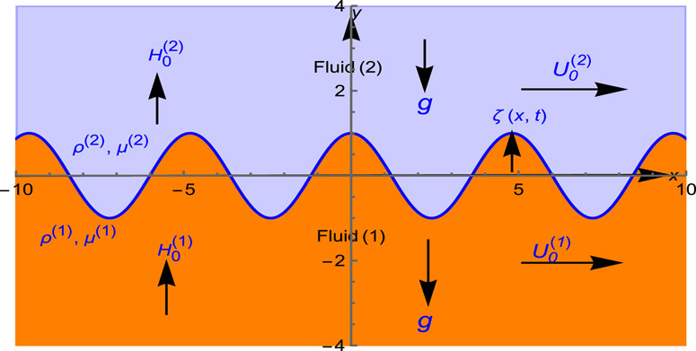
Figure 1. Sketch the physical model of the structure.

Interfacial instability can occur due to a variety of variables, including shear effects produced by velocity differences, magnetic field fluctuations that alter pressure distribution, and fractal effects that influence wave propagation. Capillary action and biological systems with fluid movement determined by viscosity and medium permeability are examples of such instabilities. In these instances, permeability is usually assumed to be constant for both non-Newtonian fluids, making the mathematical analysis easier. The study employs a two-dimensional Cartesian coordinate system (x,y), with the x-axis horizontally aligned between the two fluid layers and the y-axis vertically orientated. The fluids in the lower and top layers have different densities ${\rho }^{\left(1\right)}$ and ${\rho }^{\left(2\right)}$ and magnetic permeabilities ${\mu }^{\left(1\right)}$ and ${\mu }^{\left(2\right)}$. The liquid layers are propelled in a positive x-direction stream by ${\mu }^{\left(1\right)}$ and ${\mu }^{\left(2\right)}$, respectively.

Because of the minor disturbance for the equilibrium state, a little elevation for the flat interface in the direction of the vertical orientation is described by Equation 1, where t is the time and x represents the horizontal spatial coordinate along the interface.

$y=\zeta \left(x,t\right),(1)$

Surface deflection refers to the rise or displacement of a contact from its initial equilibrium position. This function provides insights into the system’s stability by quantifying how an external disturbance affects the interface, causing it to deviate from its flat, undisturbed state. One approach to defining the increment function as in Equation 2 [33]:

$\zeta \left(x;t\right)=\eta \left(t\right)\cos kx.(2)$

The arbitrary function $\eta \left(t\right)$ governs the amplitude of the interface disturbance, while k determines the spatial frequency of the disturbance (wavenumber). Studying this relationship enables an examination of the system’s response to perturbations, which is highly valuable for predicting interfacial behaviors in fluid dynamics and material science applications. Assume that the Dirichlet boundary condition stated below Equation 3:

$\zeta \left(0,t\right)=\eta \left(t\right),(3)$

Considering there are two initial conditions (see Equation 4) for the function $\eta \left(t\right)$

$\eta \left(0\right)=A\text{\hspace{0.5em}and\hspace{0.17em}}\dot{\eta }\left(0\right)=0(4)$

where A refers to the magnitude of the original disturbance. The normal mode technique displays the increase of a disturbance at the contact as Equation 5:

$\zeta \left(x,t\right)=\eta \left(t\right)e^{ikx}+c.c.(5)$

The complex conjugate terms (c.c) are utilized in mathematical analysis to facilitate the study of interfacial responses in two-phase systems. They enable the use of complex exponentials to represent temporal and spatial variations in interface increments, simplifying differentiation and integration in stability analysis. This notation is commonly applied in fluid dynamics, wave phenomena, and stability analysis [33].

The formula $S\left(x,y;t\right)=y-\zeta \left(x;t\right)$ represents the interface equation. The unit outward normal perpendicular to the surface interface can be described as Equation 6 [43]:

$\underline{n}=\frac{\nabla S}{\left|\nabla S\right|}=\left(-ik\zeta {\underline{e}}_x+{\underline{e}}_y\right){\left(1-k^2{\zeta }^2\right)}^{-1l2},(6)$

Bingham fluids move according to the Bingham plastic model, which describes the connection between shear stress and shear rate in viscoplastic materials. According to this model, a Bingham fluid acts like a rigid body at low shear stresses but becomes a viscous fluid when the applied shear stress surpasses a particular yield stress. The constitutive equation for a Bingham fluid is written as Equation 7 [44]:

$\varsigma ={\varsigma }_0+{\mu }_p\dot{\gamma },(7)$

where $\varsigma$ is the shear stress, ${\varsigma }_0$ yield stress, ${\mu }_p$ plastic viscosity, and $\dot{\gamma }$ shear rate. This equation states that the fluid will not deform (i.e., $\dot{\gamma }$ = 0) unless the applied shear stress $\varsigma$ exceeds the yield stress ${\varsigma }_0$. When this threshold is exceeded, the fluid flows with viscosity ${\mu }_p$. Materials that exhibit this tendency include toothpaste, mayonnaise, and certain drilling muds.

2.1 Governing equations of motion

The Bingham plastic idea has been demonstrated to appropriately reflect numerous fluids found in porous media [44]. As a result, Bingham fluid motion can be described using Cauchy’s mass and momentum conservation equations:

$\rho \left[\frac{\mathrm{\partial }\underline{V}}{\mathrm{\partial }t}+\left(\underline{V}.\nabla \right)\underline{V}\right]=-\nabla P+\nabla .\underline{\sigma }-\rho \underline{g}{\underline{e}}_y+\underline{J}\wedge \underline{B}-\frac{{\mu }_p}{\beta }\underline{V},(8)$

and the continuity Equation 9

$\nabla .{\underline{V}}_j=0,(9)$

where $\underline{V}$ is the velocity vector, $\underline{\sigma }$ is the fluid stress tensor, P is the hydrodynamic pressure and $\underline{J}$ is the electric current density.

The total, hydrodynamic, and magnetic stress tensors can be expressed as Equations 10, 11:

${\sigma }_{ij}={\sigma }_{ij}^{hydro}+{\sigma }_{ij}^{mag}(10)$

${\sigma }_{ij}^{hydro}=-P^{\left(j\right)}{\delta }_{ij}+\left({\varsigma }_0^{\left(j\right)}+{\mu }_p^{\left(j\right)}\dot{\gamma }\right),\text{and}{\sigma }_{ij}^{mag}=-H_i{B}_j-\frac{1}{2}\epsilon H_j^2{\delta }_{ij}.(11)$

Newtonian fluids are widely known for having a constant viscosity that does not change with applied stress or shear rate, resulting in a linear relationship between stress and strain rate that passes through the origin. In contrast, Bingham fluids have a yield stress, which means that a specific level of stress must be exceeded before flow occurs. Other non-Newtonian fluids include dilatant (shear-thickening) fluids, in which viscosity increases as shear rates climb (e.g., cornstarch in water), and pseudoplastic (shear-thinning) fluids, in which viscosity falls with rising shear rate. The Bingham fluid model is unique in that it encompasses the concept of yield stress, unlike many other non-Newtonian fluids that have a continuous relationship between stress and strain rate but no defined yield point.

The fundamental theory of motion is developed using the viscous potential theory (VPT), which incorporates the Brinkman-Darcy equation as well as fluid flow in porous media. Fluids are regarded as irrotational in VPT, and the derivations presented in this study are consistent with VPT concepts. The viscoelastic effects are analyzed through the application of Brownian motions, along with the primary governing equations for typical fluid phases exhibiting viscoelastic behavior.

The generalized Ohm’s law equations are expressed by Equations 12, 13 [45]:

$\underline{J}={\epsilon }_H\left(\underline{E}+\underline{V}\wedge \underline{B}\right),(12)$

and

$\nabla .\underline{B}=0,\text{and}\nabla \wedge \underline{E}=\underline{0},(13)$

where ${\epsilon }_H$ is the electrical conductivity and $\underline{E}$ represents the intensity of the electric field. We ignore the effects of ionized gas polarization and assume that the electric field vector (EF) is zero. This assumption simplifies the research by removing external influences and ionization-related issues. When the EF vector is set to zero, the governing equations only explain the travel and behavior of charged particles through internal mechanisms. This strategy is frequently used in theoretical studies to reduce system complexity and focus on certain phenomena without interference from other sources.

It is generally known that a quasi-static approximation can be used in MHD. This approximation assumes that dynamic magnetic forces have negligible influence, resulting in an irrotational magnetic field (MF) that lacks curl. The MF can be represented as a gradually varying magnetic scalar potential χ(x, y, t). The magnetic scalar potentials must meet Laplace’s equation, which determines their spatial distribution within the system, to satisfy the bulk equations ($\nabla \wedge {\underline{H}}_0^{\left(j\right)}=\underline{0}$). Thus, when the separation surface is disturbed, the MF is stated in Equations 14, 15 [46]:

${\underline{B}}^{\left(j\right)}=B_0^{\left(j\right)}{\underline{e}}_y-\nabla {\chi }^{\left(j\right)}\left(x,y;t\right),(14)$

${\nabla }^2{\chi }^{\left(j\right)}\left(x,y;t\right)=0.(15)$

The distribution of the magnetic potential ${\chi }^{\left(j\right)}\left(x,y;t\right)$ may be exhibited as:

${\chi }^{\left(1\right)}\left(x,y;t\right)=q^{\left(1\right)}\left(t\right)e^{k\left(ix+y\right)},-\infty \le y\le \zeta ,(16)$

${\chi }^{\left(2\right)}\left(x,y;t\right)=q^{\left(2\right)}{e}^{k\left(ix-y\right)},\zeta \le y\le \infty ,(17)$

where $q^{\left(j\right)}\left(t\right)$ must be determined using the applicable boundary criteria.

The expression for the equilibrium state is given in Equations 18, 19

$P_0^{\left(j\right)}=-{\rho }^{\left(j\right)}gy-\left(\frac{{\mu }_p^{\left(j\right)}}{\beta }+{\epsilon }_H^{\left(j\right)}{B}_0^{\left(j\right)2}\right)U_0^{\left(j\right)}x+C_0^{\left(j\right)},(18)$

where

$\begin{array}{l}{C}_0^{\left(1\right)}-C_0^{\left(2\right)}={\varsigma }_0^{\left(1\right)}-{\varsigma }_0^{\left(2\right)}-\left({\rho }^{\left(1\right)}-{\rho }^{\left(2\right)}\right)gy-\frac{1}{2}\left({\epsilon }^{\left(1\right)}{H}_0^{\left(1\right)2}-{\epsilon }^{\left(2\right)}{H}_0^{\left(2\right)2}\right)\\ -\left(\left(\frac{{\mu }_p^{\left(1\right)}}{\beta }+{\epsilon }_H^{\left(1\right)}{B}_0^{\left(1\right)2}\right)U_0^{\left(1\right)}-\left(\frac{{\mu }_p^{\left(2\right)}}{\beta }+{\epsilon }_H^{\left(2\right)}{B}_0^{\left(2\right)2}\right)U_0^{\left(2\right)}\right)x.\end{array}(19)$

Because of the slight disturbance, the full velocity can be represented as a potential ψ function of x, y, and t by Equations 20, 21:

${\underline{V}}^{\left(j\right)}=U_0^{\left(j\right)}{\underline{e}}_x+\nabla {\psi }^{\left(j\right)}=\left(U_0^{\left(j\right)}+ik{\psi }^{\left(j\right)}\right){\underline{e}}_x+\frac{\mathrm{\partial }{\psi }^{\left(j\right)}}{\mathrm{\partial }y}{\underline{e}}_y.(20)$

The potential ψ must meet the following Laplace equation:

${\nabla }^2{\psi }^{\left(j\right)}\left(x,y;t\right)=0.(21)$

The distribution of the potential velocity function ${\psi }^{\left(j\right)}\left(x,y;t\right)$ can be expressed as

${\psi }^{\left(1\right)}\left(x,y;t\right)={\mathrm{\Lambda }}^{\left(1\right)}\left(t\right)e^{k\left(ix+y\right)},-\infty \le y\le \zeta ,(22)$

${\psi }^{\left(2\right)}\left(x,y;t\right)={\mathrm{\Lambda }}^{\left(2\right)}\left(t\right)e^{k\left(ix-y\right)},\zeta \le y\le \infty ,(23)$

where ${\mathrm{\Lambda }}^{\left(j\right)}\left(t\right)$ is determined with the required boundary condition.

The pressure function $P^{\left(j\right)}\left(x,y;t\right)$ can be expressed as follows, based on the equation of motion (2) and the velocity potential ${\psi }^{\left(j\right)}\left(x,y;t\right)$:

$P^{\left(j\right)}\left(x,y;t\right)=-{\rho }^{\left(j\right)}gy-{\rho }^{\left(j\right)}\frac{\mathrm{\partial }}{\mathrm{\partial }t}{\psi }^{\left(j\right)}\left(x,y;t\right)-\left(\frac{{\mu }_p^{\left(j\right)}}{\beta }+{\epsilon }_H{B}_0^{\left(j\right)2}\right){\psi }^{\left(j\right)}\left(x,y;t\right).(24)$

2.2 Boundary conditions

To accurately analyze liquid inflow and its interactions with the magnetic field (MF), it is essential to determine both the hydrodynamic and magnetic stresses precisely. The boundary conditions (BCs) necessary for this computation are derived from well-established formulations [33, 44–46] and play a crucial role in defining the system’s behavior at its limits. Equations 25–27 representes BCs ensure that the physical laws regulating the interaction between the liquid and the MF are correctly applied by imposing the required limits on the system’s stress distribution. Consequently,

${\zeta }_t+ik\left(U_0^{\left(j\right)}+ik{\psi }^{\left(j\right)}\right)\zeta =\frac{\mathrm{\partial }{\psi }^{\left(j\right)}}{\mathrm{\partial }y},aty=\zeta ,(25)$

$\underline{n}\wedge \left({\underline{H}}_0^{\left(1\right)}-{\underline{H}}_0^{\left(2\right)}\right),aty=\zeta ,(26)$

and

$\underline{n}.\left({\epsilon }^{\left(1\right)}{\underline{H}}_0^{\left(1\right)}-{\epsilon }^{\left(2\right)}{\underline{H}}_0^{\left(2\right)}\right)=0,aty=\zeta .(27)$

Applying these conditions to the solutions Equations 16, 17, 22, 23 results in Equations 28–31

${\chi }^{\left(1\right)}\left(x,y;t\right)=\frac{k{\epsilon }^{\left(2\right)}\left(H_0^{\left(1\right)}-H_0^{\left(2\right)}\right)\zeta e^{k\left(y-\zeta \right)}}{k\left(1+k\zeta \right)\left({\epsilon }^{\left(1\right)}+{\epsilon }^{\left(2\right)}\right)},(28)$

${\chi }^{\left(2\right)}\left(x,y;t\right)=-\frac{k{\epsilon }^{\left(1\right)}\left(H_0^{\left(1\right)}-H_0^{\left(2\right)}\right)\zeta e^{k\left(\zeta -y\right)}}{k\left(1-k\zeta \right)\left({\epsilon }^{\left(1\right)}+{\epsilon }^{\left(2\right)}\right)},(29)$

${\psi }^{\left(1\right)}\left(x,y;t\right)=\frac{\left({\zeta }_t+ik{U}_0^{\left(1\right)}\zeta \right)}{k\left(1+k\zeta \right)}{e}^{k\left(y-\zeta \right)},(30)$

${\psi }^{\left(2\right)}\left(x,y;t\right)=-\frac{\left({\zeta }_t+ik{U}_0^{\left(2\right)}\zeta \right)}{k\left(1-k\zeta \right)}{e}^{k\left(\zeta -y\right)}.(31)$

As a consequence, the pressure distribution given in Equation 24 results in Equations 32, 33

$P^{\left(1\right)}\left(x,y;t\right)=-{\rho }^{\left(1\right)}gy-\frac{e^{k\left(y-\zeta \right)}}{k\left(1+k\zeta \right)}\left({\rho }^{\left(1\right)}||\left({\zeta }_{tt}+ik{U}_0^{\left(1\right)}{\zeta }_t\right)|+|\left(\frac{{\mu }_p^{\left(1\right)}}{\beta }+{\epsilon }_H{B}_0^{\left(1\right)2}\right)|||\left({\zeta }_t+ik{U}_0^{\left(1\right)}\zeta \right)\right),(32)$

$P^{\left(2\right)}\left(x,y;t\right)=-{\rho }^{\left(2\right)}gy+\frac{e^{k\left(\zeta -y\right)}}{k\left(1-k\zeta \right)}\left({\rho }^{\left(2\right)}||\left({\zeta }_{tt}+ik{U}_0^{\left(2\right)}{\zeta }_t\right)|+|\left(\frac{{\mu }_p^{\left(2\right)}}{\beta }+{\epsilon }_H{B}_0^{\left(2\right)2}\right)|||\left({\zeta }_t+ik{U}_0^{\left(2\right)}\zeta \right)\right).(33)$

The boundary condition indicates that surface tension ${\sigma }_T$ induces a discontinuity in the perpendicular component of the stress tensor at the interface, resulting from differential strains across the contact [43]. This discontinuity arises due to the equilibrium between fluid forces and surface tension at the interface.

$k^2{\zeta }^2\left({\sigma }_{11}^{\left(1\right)}-{\sigma }_{11}^{\left(2\right)}\right)+2ik\zeta \left({\sigma }_{21}^{\left(1\right)}-{\sigma }_{21}^{\left(2\right)}\right)-\left({\sigma }_{22}^{\left(1\right)}-{\sigma }_{22}^{\left(2\right)}\right)=-k^2{\sigma }_T\zeta {\left(1-k^2{\zeta }^2\right)}^{-1/2},y=\zeta .(34)$

The preceding solutions, along with condition Equation 34, can be used to derive the nonlinear discriminant equation after some straightforward computations.

To simplify and handle the problem, a non-dimensional analysis may be applied. Several dimensionless physical parameters are derived and listed below:

The Weber numeral: $We={\rho }_1{U}_1^{2}L/{\sigma }_T,$

The Darcy numeral: $Da=\beta /L^2,$

The Bond numeral: $B_d={\rho }_{1}g{L}^2/{\sigma }_T,$

The Bingham parameter: $B_g={\varsigma }_0^{\left(1\right)}L{\left({\mu }_p^{\left(1\right)}{U}_0^{\left(1\right)}\right)}^{-1},$

The Hartman numeral: $H{a}^2={\epsilon }_H{L}^2{B}_0^{\left(1\right)}{B}_0^{\left(2\right)}/{\mu }_p^{\left(1\right)},$

The Ohnesorge numeral: $Z={\mu }_p^{\left(1\right)}/\sqrt{{\rho }^{\left(1\right)}{\sigma }_{T}L},$

The Magnetic Bond numeral: $H=\sqrt{L{\epsilon }^{\left(1\right)}{H}_0^{\left(1\right)}{H}_0^{\left(2\right)}/{\sigma }_T}.$

Further, some helpful physical ratios are listed below:

$\rho ={\rho }^{\left(2\right)}/{\rho }^{\left(1\right)},\epsilon ={\epsilon }^{\left(2\right)}/{\epsilon }^{\left(1\right)},U=U_0^{\left(2\right)}/U_0^{\left(1\right)},\mu ={\mu }_p^{\left(2\right)}/{\mu }_p^{\left(1\right)}\text{and}{\varsigma }_0={\varsigma }_0^{\left(2\right)}/{\varsigma }_0^{\left(1\right)},{\rho }^{*}=\left(\frac{\rho -1}{\rho +1}\right).$

3 The nonlinear discriminant equation

The objective at this stage is to analyze the system’s nonlinear characteristic equation, which provides insight into its stability and dynamic behavior. This characteristic equation is derived from Equation 34 and is expressed as:

$\left(1+k{\rho }^{*}\zeta +k^2{\zeta }^2\right){\zeta }_{tt}+\left(\left(a_1+i{b}_1\right)||\left(1+k^2{\zeta }^2\right)|+|\left(a_2+i{b}_2\right)||\zeta \right){\zeta }_t+\left(a_3+i{b}_3\right)\zeta +\left(a_4+i{b}_4\right){\zeta }^2+\left(a_5+i{b}_5\right){\zeta }^3=0,(35)$

The coefficients $a_j\text{\hspace{0.17em}and\hspace{0.17em}}{b}_j$ have been expressed in non-dimensional form and are listed in the Appendix.

Rewriting complex coefficients in polar form provides a more intuitive framework for analyzing oscillations, phase correlations, and stability in systems like those described in Equation 35. Consequently, the complex coefficients in Equation 35 can be expressed in polar form as represents in Equations 36, 37

$a_j+i{b}_j=r_j{e}^{i{\theta }_j},(36)$

where the phase ${\theta }_j$ and amplitude $a_j$ are defined as

$r_j=\sqrt{a_j^2+b_j^2\text{and}}{\theta }_j={\tan }^{-1}\left(\frac{b_j}{a_j}\right)(37)$

Thus, it becomes essential to represent the complex coefficients in Equation 35 in a more descriptive form. This allows for a clearer understanding of their behavior and facilitates the analysis of their contribution to the system’s dynamics:

$\left(1+k{\rho }^{*}\zeta +k^2{\zeta }^2\right){\xi }_{tt}+\left(\left(1+k^2{\zeta }^2\right)||r_1||e^{i{\theta }_1}|+||r_2||e^{i{\theta }_2}||\zeta \right){\zeta }_t+r_3{e}^{i{\theta }_3}\zeta +r_4{e}^{i{\theta }_4}{\zeta }^2+r_5{e}^{i{\theta }_5}{\zeta }^3=0.(38)$

When the complex conjugate of Equation 38 is added to the equation itself, the real part of the coefficients is preserved, while the imaginary part is eliminated. This process ensures that the coefficients become purely real, thereby simplifying the equation’s structure and making it more straightforward to interpret and solve.

$\left(1+k{\rho }^{*}\zeta +k^2{\zeta }^2\right){\zeta }_{tt}+\left(\left(1+k^2{\zeta }^2\right)||r_1||\cos |{\theta }_1|+||\zeta |r_2||\cos |{\theta }_2\right){\zeta }_t+\left(r_3\cos {\theta }_3\right)\zeta +\left(r_4\cos {\theta }_4\right){\zeta }^2+\left(r_5\cos {\theta }_5\right){\zeta }^3=0.(39)$

Because this equation is a partial differential equation involving two independent variables, x, and t, but contains derivatives only concerning t, it is advantageous to rewrite Equation 39 using the boundary condition (3). This reformulation simplifies the equation as follows:

$\left(1+k{\rho }^{*}\eta +k^2{\eta }^2\right)\ddot{\eta }+\left(\left(1+k^2{\eta }^2\right)||r_1||\cos |{\theta }_1|+||\eta |r_2||\cos |{\theta }_2\right)\dot{\eta }+\left(r_3\cos {\theta }_3\right)\eta +\left(r_4\cos {\theta }_4\right){\eta }^2+\left(r_5\cos {\theta }_5\right){\eta }^3=0.(40)$

The simplified Equation 40 is a nonlinear ordinary differential equation involving a single variable. Its structure resembles that of a Van der Pol equation, characterized by its nonlinearity.

To adapt this nonlinear equation to fractal space characteristics, we assume that Equation 40 possesses a total frequency Ω. Utilizing this assumption, we employ the following definition in Equation 41 [47]:

${\tau }^{\alpha }=\mathrm{\Omega }t,(41)$

where $\alpha$ is a fraction power defined as $0<\alpha \le 1.$ For the specific case of $\alpha \to 1$ the classical Lindstedt-Poincaré transformation arises. As a result, the following transformations are necessary:

Accordingly, the definition of the fraction power (α), the following transformations are required.

$\dot{\eta }\left(t\right)=\frac{\mathrm{\partial }\eta }{\mathrm{\partial }{\tau }^{\alpha }}\frac{\mathrm{\partial }{\tau }^{\alpha }}{\mathrm{\partial }t}\to \mathrm{\Omega }\frac{d\eta }{d{\tau }^{\alpha }},(42)$

Consequently, we have

$\ddot{\eta }\left(t\right)\to {\mathrm{\Omega }}^2\frac{d^2\eta }{d{\tau }^{2\alpha }}.(43)$

In the situation of α→1, the classical Lindstedt-Poincaré transformation is applicable. Assuming that the derivative concerning the new variable ${\tau }^{\alpha }$ follows He’s fractal derivative formulation [46, 48, 49], this generalization extends the classical derivative to incorporate non-local or fractal-like characteristics. He’s fractal derivative approach allows the fractional derivative of order α\alphaα to capture complex multi-scale processes, such as memory effects or anomalous diffusion, which cannot be adequately described using classical calculus. As a specialized form of fractional derivative, He’s fractal derivative is frequently applied to dynamic systems exhibiting fractal properties. The derivative can take on non-integer orders (α), providing a framework that bridges the gap between purely local (integer-order) and non-local (fractional-order) dynamics.

As a result of transformations Equations 42, 43, Equation 40 takes on the fractal derivative form as

$\begin{array}{l}{\mathrm{\Omega }}^2\left(1+k{\rho }^{*}\eta +k^2{\eta }^2\right)\frac{d^2\eta }{d{\tau }^{2\alpha }}+\mathrm{\Omega }\left(r_1\cos {\theta }_1\left(1+k^2{\eta }^2\right)+\eta r_2\cos {\theta }_2\right)\frac{d\eta }{d{\tau }^{\alpha }}\\ +\left(r_3\cos {\theta }_3\right)\eta +\left(r_4\cos {\theta }_4\right){\eta }^2+\left(r_5\cos {\theta }_5\right){\eta }^3=0.\end{array}(44)$

When the transformation in Equation 42 is applied to the initial conditions given by Equation 8, the corresponding fractal initial conditions can be expressed as

$\eta \left(0\right)=A\text{and}\frac{d\eta \left(0\right)}{d{\tau }^{\alpha }}=0.(45)$

Fractal derivatives offer a versatile mathematical framework applicable to a wide range of real-world phenomena, including astronomical events, geophysical fluxes, plasma physics, and industrial processes like inertial confinement fusion. These derivatives are particularly valuable for modeling systems that exhibit memory effects, anomalous diffusion, or multi-scale behaviors—dynamics that traditional integer-order derivatives fail to capture effectively.

3.1 The process of converting the fractal into a cubic nonlinear equation

The nonlinear frequency of the system is primarily determined by the cubic nonlinearity of the restoring components, meaning that the quadratic nonlinearity does not contribute directly to the frequency structure. To address this limitation, a novel representation has been developed to reconfigure the quadratic nonlinearity while preserving the fundamental dynamics of the original nonlinear system [50]. This strategy provides a more practical way to comprehend the system’s behavior. El-Dib [51, 52] previously introduced a quadratic stiffness factor into the restoring force to compute the system’s frequency and create a solution that considers the effects of quadratic nonlinearity During variable integration, a cubic term was used to replace the quadratic component. Which enabled the system dynamics to better reflect the effect of quadratic nonlinearity. Consequently, Equation 44 can be rewritten as in Equation 46 to reflect the restoring force regulated by the quadratic nonlinearity:

$\begin{array}{l}{\mathrm{\Omega }}^2\left(1+\left(k^2+\frac{1}{2}k{\rho }^{*}\right){\eta }^2\right)\frac{d^2\eta }{d{\tau }^{2\alpha }}\\ +\mathrm{\Omega }\left(r_1\cos {\theta }_1\left(1+k^2{\eta }^2\right)+\frac{1}{2}{\eta }^2{r}_2\cos {\theta }_2\right)\frac{d\eta }{d{\tau }^{\alpha }}\\ +\left(r_3\cos {\theta }_3\right)\eta +\frac{1}{3}\left(r_4\cos {\theta }_4+3r_5\cos {\theta }_5\right){\eta }^3=0.\end{array}(46)$

This modification helps to comprehend the nonlinear Equation 44. The quadratic nonlinearities that contribute to the restoring force are transformed into an equivalent cubic effect or strategically controlled. This reconfiguration creates a more dynamically correct and analytically manageable model of the system, allowing for a better understanding of its oscillatory behavior. The above nonlinear equation can be converted into its corresponding linearized form using the method described in El-Dib’s review paper [53]. The linearized form can be generated as follows:

${\mathrm{\Omega }}^{2}a\frac{d^2\eta }{d{\tau }^{2\alpha }}+\mathrm{\Omega }b\frac{d\eta }{d{\tau }^{\alpha }}+c\eta =0.(47)$

As is typical for the linearization procedure, a trial solution matching to Equation 47 and its initial conditions Equation 45 can be obtained as

${\eta }_0\left(\tau \right)=A\cos \mathrm{\Omega }{\tau }^{\alpha }.(48)$

Following the contents of El-Dib’s review work [53] and based on the trial solution Equation 48, the coefficients in Equation 47 are computed in Equations 49–51 as:

$a=\frac{{\displaystyle {\int }_0^T}\left(1+\left(k^2+\frac{1}{2}k{\rho }^{*}\right){\eta }_0^2\right){\eta }_0^{2}d{\tau }^{\alpha }}{{\displaystyle {\int }_0^T}{\eta }_0^{2}d{\tau }^{\alpha }}=A^2\left(\frac{3}{4}+\frac{5}{8}{A}^2{k}^2+\frac{5}{16}{A}^{2}k{\rho }^{*}\right);T=\frac{2\pi }{\mathrm{\Omega }},(49)$

$b=\frac{{\displaystyle {\int }_0^T}\left(r_1\cos {\theta }_1\left(1+k^2{\eta }_0^2\right)+\frac{1}{2}{\eta }_0^2{r}_2\cos {\theta }_2\right){\left(\frac{d{\eta }_0}{d{\tau }^{\alpha }}\right)}^{2}d{\tau }^{\alpha }}{{\displaystyle {\int }_0^T}{\left(\frac{d{\eta }_0}{d{\tau }^{\alpha }}\right)}^{2}d{\tau }^{\alpha }}=\left(1+\frac{1}{4}{A}^2{k}^2\right)r_1\cos {\theta }_1+\frac{1}{8}{A}^2{r}_2\cos {\theta }_2,(50)$

$c=\frac{{\displaystyle {\int }_0^T}\left(\left(r_3\cos {\theta }_3\right)+\frac{1}{3}\left(r_4\cos {\theta }_4+3r_5\cos {\theta }_5\right){\eta }_0^2\right){\eta }_0^{2}d{\tau }^{\alpha }}{{\displaystyle {\int }_0^T}{\eta }_0^{2}d{\tau }^{\alpha }}=r_3\cos {\theta }_3+\frac{1}{4}{A}^2{r}_4\cos {\theta }_4+\frac{3}{4}{A}^2{r}_5\cos {\theta }_5.(51)$

The study of the linearized form presented in Equation 47 assesses the system frequency by Equation 52 as

${\mathrm{\Omega }}^4=\frac{4ac-b^2}{4a^2}.(52)$

Incorporating the feedback value of Ω into Equation 47 provides a more accurate formulation that considers the system’s altered frequency response. This phase is crucial for ensuring consistency with the nonlinear framework, particularly for methods like the Lindstedt-Poincaré transformation, which aims to improve solution accuracy. Using the value of Ω makes Equation 47 more understandable, allowing for additional investigation into system behavior.

$\frac{d^2\eta }{d{\tau }^{2\alpha }}+\left(\frac{b\sqrt{2a}}{a{\left(4ac-b^2\right)}^{\frac{1}{4}}}\right)\frac{d\eta }{d{\tau }^{\alpha }}+\left(\frac{2c}{\sqrt{\left(4ac-b^2\right)}}\right)\eta =0.(53)$

A crucial step in the analysis Equation 47 is converting the fractal model into its continuous-space counterpart. A promising approach involves leveraging the methods outlined in the recent work of El-Dib et al. [54, 55]. Building on these findings, the following solution is proposed to address this challenge effectively:

$\frac{d\eta }{d{\tau }^{\alpha }}={\delta }^{\alpha -1}\sin \left(\frac{1}{2}\pi \alpha \right)\frac{d\eta }{d\tau }+{\delta }^{\alpha }\cos \left(\frac{1}{2}\pi \alpha \right)\eta .(54)$

Consequently, the second derivative can be expressed as

$\frac{d^2\eta }{d{\tau }^{2\alpha }}={\delta }^{2\alpha -2}{\sin }^2\left(\frac{1}{2}\pi \alpha \right)\frac{d^2\eta }{d{\tau }^2}+2{\delta }^{\alpha }\sin \left(\frac{1}{2}\pi \alpha \right)\cos \left(\frac{1}{2}\pi \alpha \right)\frac{d\eta }{d\tau }+{\delta }^{2\alpha }{\cos }^2\left(\frac{1}{2}\pi \alpha \right)\eta .(55)$

Substituting (Equations 54, 55) into the Equation 53 reduces it to

$\frac{d^2\eta }{d{\tau }^2}+{\mu }_{eq}\frac{d\eta }{d\tau }+{\omega }_{eq}^2\eta =0.(56)$

Equation 56 represents a simplified damped harmonic linear equation with the following Equation 57 that corresponding initial conditions:

$\eta \left(0\right)=A\text{and}\frac{d\eta \left(0\right)}{d\tau }=-\delta \cot \left(\frac{1}{2}\pi \alpha \right)A.(57)$

The coefficients appearing in Equation 56 are listed as follows:

${\mu }_{eq}=\frac{2\delta }{\sqrt{2a}{\left(4ac-b^2\right)}^{\frac{1}{4}}{\delta }^{\alpha }\sin \left(\frac{1}{2}\pi \alpha \right)}\left(b+\sqrt{2a}{\left(4ac-b^2\right)}^{\frac{1}{4}}\delta \cos \left(\frac{1}{2}\pi \alpha \right)\right),(58)$

${\omega }_{eq}^2=\frac{{\delta }^2}{a{\delta }^{2\alpha }{\sin }^2\left(\frac{1}{2}\pi \alpha \right)}\left(a|{\delta }^{2\alpha }||{\cos }^2||\left(\frac{1}{2}\pi \alpha \right)|+|b|\sqrt{2a}||{\left(4ac-b^2\right)}^{-\frac{1}{4}}||{\delta }^{\alpha }||\cos \left(\frac{1}{2}\pi \alpha \right)|+||2|a|c|{\left(4ac-b^2\right)}^{-\frac{1}{2}}\right).(59)$

The solution to Equation 56 is given in the following form:

$\eta \left(\tau \right)=A{e}^{-\frac{1}{2}{\mu }_{eq}\tau }\left(\cos \mathrm{\Omega }\tau +\frac{1}{2\mathrm{\Omega }}\left({\mu }_{eq}-2\delta \cot \left(\frac{1}{2}\pi \alpha \right)\right)\sin \mathrm{\Omega }\tau \right),(60)$

where the total frequency Ω, corresponding to the above fractal solution, is determined as:

${\mathrm{\Omega }}^2={\omega }_{eq}^2-\frac{1}{4}{\mu }_{eq}^2.(61)$

By adding Equations 58, 59 to Equation 61, the system frequency Ω is formulated in terms of the fractal parameter δ and the fractal order α. This formulation establishes a direct relationship between the system’s oscillatory behavior and its fractal characteristics, enabling a deeper understanding of how fractal properties influence stability and frequency dynamics.

${\mathrm{\Omega }}^2=\frac{{\delta }^2}{a{\delta }^{2\alpha }{\sin }^2\left(\frac{1}{2}\pi \alpha \right)}\left\{a\left({\delta }^{2\alpha }-{\delta }^2\right)|{\cos }^2||\left(\frac{1}{2}\pi \alpha \right)|+|b|\sqrt{2a}||{\left(4ac-b^2\right)}^{-\frac{1}{4}}||\left({\delta }^{\alpha }-\delta \right)||\cos \left(\frac{1}{2}\pi \alpha \right)|+|\frac{1}{2}||{\left(4ac-b^2\right)}^{\frac{1}{2}}\right\}.(62)$

It is important to note that an unknown parameter, δ, remains present in the above frequency formula. To determine this unknown, we compare the original characteristic Equation 53, which governs the system’s state before applying the transformations Equations 54, 55, to the characteristic equation in its standard derivative form, as represented by Equation 56. This comparison allows us to bridge the fractal formulation with the conventional approach. To achieve this, two key comparisons are necessary: one analyzing the damping behavior and the other comparing the natural frequencies in Equations 53, 56. The results of these comparisons lead to the following conclusions:

$b{\delta }^{\alpha }\sin \left(\frac{1}{2}\pi \alpha \right)=\delta \left(b+\sqrt{2a}{\left(4ac-b^2\right)}^{\frac{1}{4}}\delta \cos \left(\frac{1}{2}\pi \alpha \right)\right),(63)$

${\delta }^{2\alpha }{\sin }^2\left(\frac{1}{2}\pi \alpha \right)=\frac{{\delta }^2{\left(4ac-b^2\right)}^{\frac{1}{2}}}{2ac}\left(a|{\delta }^{2\alpha }||{\cos }^2||\left(\frac{1}{2}\pi \alpha \right)|+|b|\sqrt{2a}||{\left(4ac-b^2\right)}^{-\frac{1}{4}}||{\delta }^{\alpha }||\cos \left(\frac{1}{2}\pi \alpha \right)|+|2|a|c|{\left(4ac-b^2\right)}^{-\frac{1}{2}}\right).(64)$

By eliminating ${\delta }^{\alpha }$ between Equations 63, 64, we derive a characterized equation for the parameter δ. This equation establishes a fundamental relationship that represents δ in terms of the system’s fractal properties. The resulting equation takes the form Equation 65:

${\delta }^3+m_2{\delta }^2+m_1\delta +m_0=0,(65)$

The third-order polynomial equation encapsulates the nonlinear influence of fractal parameters on the system’s stability and frequency dynamics. This formulation provides deeper insights into how fractal conditions affect the system’s overall behavior. The coefficients m’s in the equation are defined in Equation 66:

$\begin{array}{l}{m}_2=\frac{2b}{\sqrt{2a}{\left(4ac-b^2\right)}^{\frac{1}{4}}\cos \left(\frac{1}{2}\pi \alpha \right)},\\ m_1=-\frac{1}{2a\sqrt{4ac-b^2}{\cos }^2\left(\frac{1}{2}\pi \alpha \right)}\\ \left(\left(4ac-b^2\right)-2b^2\sin \left(\frac{1}{2}\pi \alpha \right)-4ac{\cos }^2\left(\frac{1}{2}\pi \alpha \right)\right),\\ m_0=\frac{4bc}{\sqrt{2a}{\left(4ac-b^2\right)}^{\frac{3}{4}}}\left(\frac{b^2}{4ac}-\sin \left(\frac{1}{2}\pi \alpha \right)\right)\frac{\sin \left(\frac{1}{2}\pi \alpha \right)}{{\cos }^3\left(\frac{1}{2}\pi \alpha \right)}.\end{array}(66)$

Stability is ensured when the right-hand side of Equation 62 remains positive. This condition guarantees that the system’s response remains bounded and does not exhibit unbounded growth, which is crucial for maintaining equilibrium and preventing instability. The transition curve that separates stable from unstable states is illustrated as ${\mathrm{\Omega }}^2=0$, requiring:

$a\left\{a\left({\delta }^{2\alpha }-{\delta }^2\right)|{\cos }^2||\left(\frac{1}{2}\pi \alpha \right)|+|b|\sqrt{2a}||{\left(4ac-b^2\right)}^{-\frac{1}{4}}||\left({\delta }^{\alpha }-\delta \right)||\cos \left(\frac{1}{2}\pi \alpha \right)|+|\frac{1}{2}||{\left(4ac-b^2\right)}^{\frac{1}{2}}\right\}=0.(67)$

4 Numerical illustration

Several graphs are plotted for the transition curve Equation 67 to illustrate the impact of the fractal dimensional parameter $\alpha$ and other key physical parameters on the system’s stability behavior. The graphs represent the transition curve that separates the stable state from the unstable one. These visual representations help analyze how variations in these parameters influence stability transitions and dynamic responses. The dimensionless numbers for this figure were chosen as follows:

$A=1,\rho =1.2,\mu =0.1,U=0.1,\epsilon =0.01,H=10,Ha=3,Z=0.01,W_e=0.5,D_a=0.01,{\varsigma }_0=0.1,B_d=0.01,B_g=0.01$

Figure 2 illustrates the stability plane $\left({\mathrm{\Omega }}^2-k\right)$ along with a graph of frequency ${\mathrm{\Omega }}^2$ versus wavenumber k. The stability behavior varies with the fractal dimension $\alpha$, where the stable region is highlighted, and the unstable region remains unshaded. It is observed that the stable region lies above the transition curve, while the unstable region is positioned below it. The graph of frequency ${\mathrm{\Omega }}^2$ against k shows that as k increases, the transition curve shifts higher, taking the shape of a negative exponential function and expanding the unstable region. Additionally, a decrease in the fractal order $\alpha$ leads to a reduction in the stable area. This effect is more pronounced for very small values of k, where the stability zone significantly shrinks as $\alpha$ decreases. This behavior indicates that an increase in the wavenumber k enhances instability, while a decrease in $\alpha$ also has a destabilizing effect on the system.

Figure 2

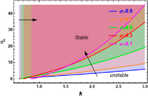
Figure 2. Demonstrate the influence of the variation of the fractal order on the stability plane $\left({\mathrm{\Omega }}^2-k\right)$.

Figure 3 illustrates the transition curve Equation 67 in the stability plane $\left({\mathrm{\Omega }}^2-\alpha \right)$ while analyzing variations in the wavenumber k for the same system considered in Figure 2. It is observed that as k increases, the unstable region expands, particularly in areas corresponding to small values of the fractal parameter alpha. This indicates that higher wavenumbers k contributes to greater instability, with the effect being more pronounced when is small. Additionally, larger values of k are associated with smaller values of alpha, leading to a more unstable response in the system. However, for higher values of alpha, the destabilizing influence of increasing k is minimal. This implies that the fractal parameter has a substantial function in determining stability, with its significance decreasing as it increases.

Figure 3

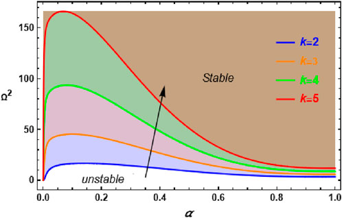
Figure 3. Demonstrate the influence of the variation of the wavenumber k on the stability plane $\left({\mathrm{\Omega }}^2-\alpha \right)$.

Figure 4 depicts an examination of the influence of the magnetic Bond number H on the stability behavior for the same system seen in Figure 2, with the wavenumber set to k = 2. The results show that raising H changes the stability behavior, such as wavenumber k, resulting in a destabilizing effect in the system. Specifically, when H increases, the unstable region widens, with the effect being most noticeable for small values of the fractal parameter $\alpha$. This shows that the magnetic field has a major destabilizing effect in regimes with low fractal dimensions. For larger α values, H has a limited impact on stability, causing only slight destabilization. This means that, while the magnetic Bond number is important in stability management, its effects reduce as the fractal parameter grows, emphasizing the interaction of magnetic forces and fractal dimension in regulating system behavior.

Figure 4

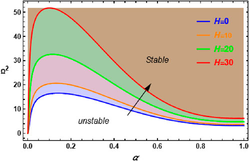
Figure 4. Demonstrate the influence of the variation of the magnetic Bond number H on the stability plane $\left({\mathrm{\Omega }}^2-\alpha \right)$.

Figure 5 depicts a study of the impact of the Hartmann number Ha on the stability plane for the identical system as in Figure 4, with the magnetic Bond number set to H = 10. This evaluation reveals how changes affect the system’s stability characteristics. An analysis of the graph shows that increasing leads the transition curve to shift downward, thereby expanding the stable region. This downward movement implies a stabilizing impact, allowing more of the system to remain stable. However, for very small values of the fractal parameter alpha, the stability region experiences only a slight reduction in its stabilizing influence. As increases, the stabilizing effect gradually diminishes, indicating that the impact of the Hartmann number is more pronounced in low-fractal-dimension regimes. Furthermore, for higher values of alpha, the stabilizing effect of Ha becomes minimal, suggesting that at larger fractal dimensions, the influence of the Hartmann number on system stability is less significant. This behavior highlights the complex interaction between magnetic forces and fractal properties in determining the stability characteristics of the system.

Figure 5

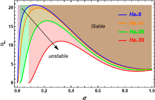
Figure 5. Demonstrate the influence of the variation of the Hartmann number Ha on the stability plane $\left({\mathrm{\Omega }}^2-\alpha \right)$.

The graph in Figure 6 illustrates the effect of the Ohnesorge number Z on the stability plane $\left({\mathrm{\Omega }}^2-\alpha \right)$. The dimensionless parameters used for this figure are identical to those in Figure 5, except that the Hartmann number is fixed at Ha = 30. This analysis provides insights into how variations in Z influence system stability. The stability behavior observed in this graph closely resembles the effects of the Hartmann number presented in Figure 5. Specifically, an increase in Z leads to a stabilizing effect, similar to what is observed with increasing Ha. As increases, the transition curve shifts downward, expanding the stable region and reinforcing the system’s resistance to perturbations. This suggests that the Ohnesorge number plays a crucial role in reducing instability by modifying the fluid’s response to external forces. Overall, the results indicate that, like the Hartmann number, the Ohnesorge number enhances stability by suppressing disturbances, making it an essential parameter in determining the behavior of the system under varying conditions.

Figure 6

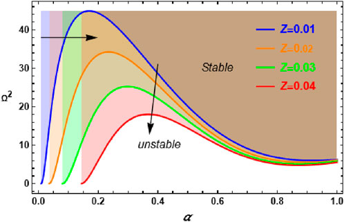
Figure 6. Demonstrate the influence of the variation of the Ohnesorge numeral Z on the stability plane $\left({\mathrm{\Omega }}^2-\alpha \right)$.

Figure 7 shows the fractal time history, showing the fractal solution Equation 60 against variations in the fractal dimensional parameter α. This graph is a schematic representation of the same system as in Figure 2, providing insight into the system’s temporal evolution under different fractal settings. The presence of a dampening feature is one of the most noticeable aspects of this image. The damping effect gets increasingly significant as the fractal parameter increases, showing that the system suppresses oscillatory instabilities more effectively over time. This shows that greater values help to improve stability by lowering fluctuations and mitigating instability. Increasing α has a stabilizing effect, as higher fractal dimensions result in more regulated and damped system responses. As a result, it not only reduces instability but also maintains overall system stability, making it an important parameter in managing the system’s dynamic behavior throughout time.

Figure 7

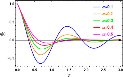
Figure 7. Represents the fractal time history as given by the analytical solution Equation 60.

Figure 8 displays the fractal time history, demonstrating how changes in the magnetic Bond number influence system behavior with the wavenumber set to k = 3. Similarly, Figure 9 shows how the wavenumber grows while the magnetic Bond number remains constant at H = 1. These computations are for the same system as seen in Figure 7, but the fractal parameter is kept constant at α = 0.1. These results provide an important finding about the influence of increasing on the system’s dynamic response. As either value grows, the cycle rate lowers, indicating that the system is becoming unstable. This implies that higher values of or contribute to a decrease in oscillation frequency, resulting in more extreme instability. The decrease in cycle rate demonstrates how the magnetic Bond number and wavenumber influence the system’s temporal evolution, emphasizing their importance in influencing stable behavior under fractal settings.

Figure 8

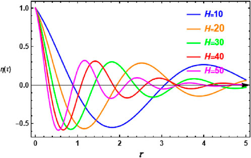
Figure 8. Represents the fractal time history for variation of H.

Figure 9

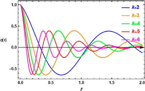
Figure 9. Represents the fractal time history for variation of k.

5 Conclusion

This study employs sophisticated nonlinear analysis techniques using Fractal analysis to control Interfacial stability of MHD Bingham Fluids in Micro-Porous MEMS Structures. The Harmonic Equivalent Linearization Method (HELM) is an important methodological tool used in this study. It simplifies the analysis by translating the nonlinear dynamical characteristic equation into an equivalent linear form. This transformation improves the analytical analysis and solution to the stability problem, making it easier to anticipate system behavior under various parametric conditions. The governing equations are stated in a fractal framework using the modified Lindstedt-Poincaré transformation, which is critical for capturing Bingham fluids’ complicated interfacial stability properties. This work incorporates fractal adjustments to account for the impacts of non-integer dimensions, providing a more accurate description of the physical system, particularly in porous and uneven media. The fractal framework provides more insight into how microstructural differences affect fluid stability, which is critical for real-world applications involving geometric complexity and diverse structures.

Several major observations emerge from the numerical and analytical findings:

1. Increasing the fractal dimension α improves system stability by adding stronger damping effects, minimizing instability, and maintaining interface stability over time.

2. Wavenumber k has a destabilizing impact, causing the unstable zone to expand, especially for lower α values.

3. Magnetic Bond Number H has a destabilizing effect, especially in low-fractal-dimension regimes, highlighting the importance of electromagnetic forces in stability modulation.

4. Hartmann Number Ha: Higher values expand the stability region by pushing the transition curve downward, decreasing instability and enhancing system stability.

5. Effects of Ohnesorge Number Z: This number has a stabilizing impact by decreasing oscillatory instabilities and expanding the stable area.

The fractal time history study shows that higher alpha values result in stronger damping effects, which increase the system’s robustness to perturbations. The combination of magnetic, hydrodynamic, and fractal properties facilitates the intricate interplay of forces that influences stability behavior in MHD Bingham fluids. Overall, this research advances our understanding of nonlinear stability in viscoelastic fluids under fractal effects and magnetic fields. The findings are relevant to industrial and geophysical applications, particularly those requiring interfacial stability, such as fluid flow in porous media, enhanced oil recovery, and biomedical engineering. Future research could extend these findings by looking into parametric effects and the nonlinear Mathieu equation contributions. Our study develops nonlinear, fractal, and MHD-based modeling techniques for MEMS structures, addressing electrostatic interactions, geometric nonlinearity, and scale-dependent effects. This methodology will be validated and expanded for microscale technologies.

Data availability statement

The original contributions presented in the study are included in the article/supplementary material, further inquiries can be directed to the corresponding author.

Author contributions

YE-D: Investigation, Software, Writing – review and editing, Supervision, Writing – original draft, Formal Analysis, Methodology. AM: Formal Analysis, Writing – original draft, Methodology. HA: Writing – original draft, Investigation, Validation.

Funding

The author(s) declare that financial support was received for the research and/or publication of this article.

Acknowledgments

The authors express their gratitude to Princess Nourah bint Abdulrahman University Researchers Supporting Project Number (PNURSP2025R17), Princess Nourah bint Abdulrahman University, Riyadh, Saudi Arabia.

Conflict of interest

The authors declare that the research was conducted in the absence of any commercial or financial relationships that could be construed as a potential conflict of interest.

Generative AI statement

The author(s) declare that Generative AI was used in the creation of this manuscript. We only used AI to improve the manuscript’s language.

Publisher’s note

All claims expressed in this article are solely those of the authors and do not necessarily represent those of their affiliated organizations, or those of the publisher, the editors and the reviewers. Any product that may be evaluated in this article, or claim that may be made by its manufacturer, is not guaranteed or endorsed by the publisher.

References

1. Yang D, Krasowska M, Craig P, Popescu MN, Ralston J. Dynamics of capillary-driven flow in open microchannels. The J Phys Chem C (2011) 115(38):18761–9. doi:10.1021/jp2065826

CrossRef Full Text | Google Scholar

2. Lade RK, Hippchen EJ, Macosko CW, Francis L. Dynamics of capillary-driven flow in 3D printed open microchannels. Langmuir (2017) 33(12):2949–64. doi:10.1021/acs.langmuir.6b04506

PubMed Abstract | CrossRef Full Text | Google Scholar

3. Tokihiro JC, Robertson IH, Gregucci D, Shin A, Michelini E, Nicholson TM, et al. The dynamics of capillary flow in an open-channel system featuring trigger valves. Sci Rep (2024) 14:31732. doi:10.1038/s41598-024-82329-3

PubMed Abstract | CrossRef Full Text | Google Scholar

4. Khanjani E, Fergola A, López JA, Nazarnezhad S, Casals-Terré J, Marasso SL, et al. Capillary microfluidics for diagnostic applications: fundamentals, mechanisms, and capillarics. Front Lab a Chip Tech (2025) 4. doi:10.3389/frlct.2025.1502127

CrossRef Full Text | Google Scholar

5. Saleh TA. Surface Science of Adsorbents and Nanoadsorbents. Properties and Applications in Environmental Remediation. Cambridge, MA: Academic Press. (2022) p. 316.

Google Scholar

6. Macgregor M, Vasilev K. Questions and answers on the wettability of nano-engineered surfaces. Adv Mater Inter (2017) 4(16):1700381. doi:10.1002/admi.201700381

CrossRef Full Text | Google Scholar

7. Squires TM, Quake SR. Microfluidics: fluid physics at the nanoliter scale. Rev Mod Phys (2005) 77:977–1026. doi:10.1103/RevModPhys.77.977

CrossRef Full Text | Google Scholar

8. Sisó G, Rosell-Mirmi J, Fernández Á, Laguna G, Vilarrubi M, Barrau J, et al. Thermal analysis of a MEMS-based self-adaptive microfluidic cooling device. Micromachines (2021) 12:505. doi:10.3390/mi12050505

PubMed Abstract | CrossRef Full Text | Google Scholar

9. Tian D, He C-H, He J-H. Fractal pull-in stability theory for microelectromechanical systems. Front Phys (2021) 9:606011. doi:10.3389/fphy.2021.606011

CrossRef Full Text | Google Scholar

10. Tian Y, Shao Y (2024). Mini-review on periodic properties of MEMS oscillators. Front Phys 12:1498185. doi:10.3389/fphy.2024.1498185

CrossRef Full Text | Google Scholar

11. He J-H, Bai Q, Luo Y-C, Kuangaliyeva D, Ellis G, Yessetov Y, et al. (2025). Modeling and numerical analysis for MEMS graphene resonator. Front Phys 13:1551969. doi:10.3389/fphy.2025.1551969

CrossRef Full Text | Google Scholar

12. Bingham EC. An investigation of the laws of plastic flow. Bull Bur Stand (1916) 13(2):309–53. doi:10.6028/bulletin.304

CrossRef Full Text | Google Scholar

13. Bingham EC. Fluidity and plasticity. New York: McGraw-Hill (1922). p. 219.

Google Scholar

14. Bird RB, Dai G, Yarusso BJ. The rheology and flow of viscoplastic materials. Rev Chem Eng (1983) 1:1–70. doi:10.1515/revce-1983-0102

CrossRef Full Text | Google Scholar

15. Yang L, Du K. A comprehensive review on the natural, forced, and mixed convection of non-Newtonian fluids (nanofluids) inside different cavities. J Therm Anal Calorim (2019) 140(10):2033–54. doi:10.1007/s10973-019-08987-y

CrossRef Full Text | Google Scholar

16. Peiguang W, Zhendong W. The analysis of stability of Bingham fluid flowing down an inclined plane. Appl Math Mech (1995) 16:1013–8. doi:10.1007/BF02538843

CrossRef Full Text | Google Scholar

17. Chhabra RP, Richardson JF. Non-Newtonian flow and applied rheology: engineering applications. Elsevier Science (2008).

Google Scholar

18. Borrelli A, Giantesio G, Patria MC. Magnetohydrodynamic flow of a Bingham fluid in a vertical channel: mixed convection. Fluids (2021) 6(4):154. doi:10.3390/fluids6040154

CrossRef Full Text | Google Scholar

19. Eslami A, Frigaard IA, Taghavi SM. Viscoplastic fluid displacement flows in horizontal channels: numerical simulations. J Non-Newtonian Fluid Mech (2017) 249:79–96. doi:10.1016/j.jnnfm.2017.10.001

CrossRef Full Text | Google Scholar

20. Ullah I, Arif M, Nadeem S, Alzabut J. Numerical computations of MHD mixed convection flow of Bingham fluid in a porous square chamber with a wavy cylinder. Int J Thermofluids (2024) 24:100938. doi:10.1016/j.ijft.2024.100938

CrossRef Full Text | Google Scholar

21. Negishi H, Kondo M, Amakawa H, Obara S, Kurose R. Bingham fluid simulations using a physically consistent particle method. J Fluid Sci Technology: Bull ASME (2023) 18(4):JFST0035–163718. doi:10.1299/jfst.2023jfst0035

CrossRef Full Text | Google Scholar

22. Kumar A, Bhardwaj A, Tripathi D. Bingham plastic fluids flow analysis in multimembranes fitted porous medium. Chin J Phys (2024) 90:446–62. doi:10.1016/j.cjph.2024.05.040

CrossRef Full Text | Google Scholar

23. Mollah MT, Rasmussen HK, Poddar S, Islam MM, Parvine M, Alam MM, et al. Ion-slip effects on Bingham fluid flowing through an oscillatory porous plate with suction. Math Model Eng. Probl. (2021) 8(5):673–81. doi:10.18280/mmep.080501

CrossRef Full Text | Google Scholar

24. Falsaperla P, Giacobbe A, Mulone G. Stability of the plane Bingham-Poiseuille flow in an inclined channel. Fluids (2020) 5(3):141. doi:10.3390/fluids5030141

CrossRef Full Text | Google Scholar

25. Gunawan AY, van de Ven AAF. Non-steady pressure-driven flow of a Bingham fluid through a channel filled with a Darcy Brinkman medium. J Eng Math (2022) 137:5. doi:10.1007/s10665-022-10244-5

CrossRef Full Text | Google Scholar

26. Talon L, Hennig AA, Hansen A, Rosso A. Influence of the imposed flow rate boundary condition on the flow of Bingham fluid in porous media. Phys Rev Fluids (2024) 9:063302. doi:10.1103/physrevfluids.9.063302

CrossRef Full Text | Google Scholar

27. Mollah MT, Poddar S, Islam MM, Alam MM. Non-isothermal Bingham fluid flow between two horizontal parallel plates with Ion-slip and Hall currents. SN Appl Sci (2021) 3:115. doi:10.1007/s42452-020-04012-2

CrossRef Full Text | Google Scholar

28. Mollah MT. EMHD laminar flow of Bingham fluid between two parallel Riga plates. Int J Heat Technol (2019) 37(2):641–8. doi:10.18280/ijht.370236

CrossRef Full Text | Google Scholar

29. Shih P-H, Do TN, Gumbs G, Huang D, Lin H, Chang TR. Quantized Hall current in a topological nodal-line semimetal under electromagnetic waves. Phys Rev B (2024) 110:085427. doi:10.1103/physrevb.110.085427

CrossRef Full Text | Google Scholar

30. Ali AHH. Impact of varying viscosity with all current on peristaltic flow of viscoelastic fluid through porous medium in irregular micro channel. Iraqi J Sci (2022) 63(3):1265–76. doi:10.24996/ijs.2022.63.3.31

CrossRef Full Text | Google Scholar

31. Qiao Y, Xu H, Qi H. Rotating MHD flow and heat transfer of generalized Maxwell fluid through an infinite plate with Hall effect. Acta Mech Sin (2024) 40:223274. doi:10.1007/s10409-023-23274-x

CrossRef Full Text | Google Scholar

32. de Franciscis S, Pascual-Granado J, Suárez JC, García Hernández A, Garrido R. Fractal analysis applied to light curves of δ Scuti stars. Monthly Notices R Astronomical Soc (2018) 481(Issue 4):4637–49. doi:10.1093/mnras/sty2496

CrossRef Full Text | Google Scholar

33. El-Dib YO. Insights into fractal space features in nonlinear electrohydrodynamic Rayleigh–Taylor instability of viscous fluids. Phys Fluids (2024) 36:122127. doi:10.1063/5.0243581

CrossRef Full Text | Google Scholar

34. Heinen M, Schnyder SK, Brady JF, Löwen H. Classical liquids in fractal dimension. Phys Rev Lett (2015) 115:097801. doi:10.1103/PhysRevLett.115.097801

PubMed Abstract | CrossRef Full Text | Google Scholar

35. Gmachowski L. Fractal model of anomalous diffusion. Eur Biophys J (2015) 44(8):613–21. doi:10.1007/s00249-015-1054-5

PubMed Abstract | CrossRef Full Text | Google Scholar

36. Kearney M. Engineered fractal cascades for fluid control applications. In: Proceedings, fractals in engineering, INRIA, arcachon, France (1997).

Google Scholar

37. Kearney M. Control of fluid dynamics with engineered fractals – adsorption, process applications. Chem Eng Comm (1999) 173:43–52. doi:10.1080/00986449908912775

CrossRef Full Text | Google Scholar

38. Feng GQ (2023). A circular sector vibration system in a porous medium: a fractal-fractional model and He’s frequency formulation. Facta Universitatis Ser Mech Eng. doi:10.22190/FUME230428025F

CrossRef Full Text | Google Scholar

39. He C-H, Liu C. Fractal Dimensions Of A Porous Concrete And Its Effect On The Concrete’s Strength. Ser Mech Eng (2023) 21:137–50. doi:10.22190/FUME221215005H

CrossRef Full Text | Google Scholar

40. Li C, Xu Y, Jiang Z, Yu B, Xu P. Fractal analysis on the mapping relationship of conductivity properties in porous material. Fractal Fract (2022) 6:527. doi:10.3390/fractalfract6090527

CrossRef Full Text | Google Scholar

41. Quan C-Q, Jiao C-J, Chen W-Z, Xue Z-C, Liang R, Chen X-F (2023). The impact of fractal gradation of aggregate on the mechanical and durable characteristics of recycled concrete. Fractal Fract. 7, 663. doi:10.3390/fractalfract7090663

CrossRef Full Text | Google Scholar

42. Viatcheslav B, Aimy B, David S, Ned D (2010). Fractal flow patterns in hydrophobic microfluidic pore networks: experimental modeling of two-phase flow in porous electrodes. arXiv:0909. doi:10.48550/arXiv.0909.0758

CrossRef Full Text | Google Scholar

43. Chandrasekhar S. Hydrodynamic and hydromagnetic stability. Oxford, United Kingdom: Oxford University Press (2000).

Google Scholar

44. Hughes WF, Brighton JA. Fluid dynamics. New York, NY: McGraw-Hill Book Company (1967).

Google Scholar

45. Melcher JR. Field coupled surface waves. Boston, MA: MIT Press (1963).

Google Scholar

46. He JH, El-Dib YO. A tutorial introduction to the two-scale fractal calculus and its application to the fractal Zhiber-Shabat oscillator. Fractals (2021) 29(8):2150268. doi:10.1142/s0218348x21502686

CrossRef Full Text | Google Scholar

47. El-Dib YO, Alyousef HA. ModifiedLindstedt-Poincare transformation for fractal resonance approach in vibration 2-DOF heterogeneous system. J Low Frequency Noise, Vibration Active Control (2025). doi:10.1177/14613484251335736

CrossRef Full Text | Google Scholar

48. He JH. A tutorial review on fractal space and fractional calculus. Int J Theor Phys (2014) 53:3698–718. doi:10.1007/s10773-014-2123-8

CrossRef Full Text | Google Scholar

49. He JH. Fractal calculus and its geometrical explanation. Results Phys (2018) 10:272–6. doi:10.1016/j.rinp.2018.06.011

CrossRef Full Text | Google Scholar

50. El-Dib YO. Insights into transferal to fractal space modeling: delayed forced Helmholtz–Duffing oscillator with the non-perturbative approach. Commun Theor Phys (2024) 77:015002. doi:10.1088/1572-9494/ad7ceb

CrossRef Full Text | Google Scholar

51. El-Dib YO. Stability analysis of a time-delayed Van der Pol-Helmholtz-Duffing oscillatorin fractal space with a non-perturbative approach. Commun Theor Phys (2024) 76:045003. doi:10.1088/1572-9494/ad2501

CrossRef Full Text | Google Scholar

52. El-Dib YO. A review of the frequency-amplitude formula for nonlinear oscillators and its advancements. J Low Freq Noise Vib Act Control (2024) 43:1032–64. doi:10.1177/14613484241244992

CrossRef Full Text | Google Scholar

53. El-Dib YO, Elgazery NS. A novel pattern in a class of fractal models with the non-perturbative approach. Chaos, Solitons Fractals (2022) 164:112694. doi:10.1016/j.chaos.2022.112694

CrossRef Full Text | Google Scholar

54. El-Dib YO, Elgazery NS. An efficient approach to converting the damping fractal models to the traditional system. Commun Nonlinear Sci Numer Simul (2023) 118:107036. doi:10.1016/j.cnsns.2022.107036

CrossRef Full Text | Google Scholar

55. El-Dib YO, Elgazery NS, Alyousef HA. The up-grating rank approach to solve the forced fractal Duffing oscillator by non-perturbative technique. Facta Univ Mech Eng (2024) 22(2):199–216. doi:10.22190/fume230605035e

CrossRef Full Text | Google Scholar

Appendix

The constants that appear in Equation 35 may be listed as:

$a_1=\frac{1}{k\left(\rho +1\right)}\left(2k^{2}Z\left(1+\mu \right)+\left(Z/D_a\right)\left(1+\mu \right)+2ZH{a}^2\right),$

$b_1=\frac{k}{\rho +1}\sqrt{W_e}\left(1+U\rho \right),$

$a_2=\frac{k}{\rho +1}\left(2Z{k}^2\left(1-\mu \right)-\frac{Z}{D_a}\left(1-\mu \right)\right),$

$b_2=-k^2\sqrt{W_e}\left(\frac{1-\rho U}{\rho +1}\right),$

$a_3=\frac{1}{\rho +1}k\left(B_d\left(1-\rho \right)-k^2-2k^3\right)-\frac{k^2}{\left(\rho +1\right)}\frac{\epsilon {\left(\epsilon -1\right)}^2}{\left(1+\epsilon \right)}{H}^2,$

$b_3=\frac{k}{\rho +1}\left(2||Z||k^2||\sqrt{W_e}||\left(1+U\mu \right)|+|\frac{Z}{D_a}||\sqrt{W_e}||\left(1+U\mu \right)|+|Z||H|a^2||\sqrt{W_e}||\left(1+U\right)|-||2||Z||B_g||\sqrt{W_e}||\left(1-{\varsigma }_0\right)\right),$

$a_4=k^{3}Z{B}_g\sqrt{W_e}\left(\frac{1-{\varsigma }_0}{\rho +1}\right)-\frac{k^3}{2\left(\rho +1\right)}\frac{\epsilon }{\left(1+\epsilon \right)}\left[\left(1-\epsilon \right)\left(3+2\epsilon +3{\epsilon }^2\right)+4\left(\epsilon -1\right)\right]H^2,$

$b_4=\frac{k^2}{\rho +1}\left(2|k^2||Z||\sqrt{W_e}||\left(1-\mu U\right)|-|Z||H|a^2||\sqrt{W_e}||\left(1-U\right)|-|\frac{Z}{D_a}||\sqrt{W_e}||\left(1-\mu U\right)\right),$

$a_5=-\frac{3k^5}{2\left(\rho +1\right)}-\frac{3}{2}\frac{k^4}{\left(\rho +1\right)}\frac{\epsilon {\left(\epsilon -1\right)}^2}{\left(1+\epsilon \right)}{H}^2,$

$b_5=\frac{k^3}{\rho +1}\left(4||Z||k^2||\sqrt{W_e}||\left(1+U\mu \right)|+|Z||H|a^2||\sqrt{W_e}||\left(1+U\right)|+|\frac{Z}{D_a}||\sqrt{W_e}||\left(1+U\mu \right)|-||4||Z||B_g||\sqrt{W_e}||\left(1-{\varsigma }_0\right)\right).$