An echo state network based on enhanced intersecting cortical model for discrete chaotic system prediction

Introduction: The prediction of chaotic time series is a persistent problem in various scientific domains due to system characteristics such as sensitivity to initial conditions and nonlinear dynamics. Deep learning models, while effective, are associated with high computational costs and large data requirements. As an alternative, Echo State Networks (ESNs) are more computationally efficient, but their predictive accuracy can be constrained by the use of simplistic neuron models and a dependency on hyperparameter tuning.

Methods: This paper proposes a framework, the Echo State Network based on an Enhanced Intersecting Cortical Model (ESN-EICM). The model incorporates a neuron model with internal dynamics, including adaptive thresholds and inter-neuron feedback, into the reservoir structure. A Bayesian Optimization algorithm was employed for the selection of hyperparameters. The performance of the ESN-EICM was compared to that of a standard ESN and a Long Short-Term Memory (LSTM) network. The evaluation used data from three discrete chaotic systems (Logistic, Sine, and Ricker) for both one-step and multi-step prediction tasks.

Results: The experimental results indicate that the ESN-EICM produced lower error metrics (MSE, RMSE, MAE) compared to the standard ESN and LSTM models across the tested systems, with the performance difference being more pronounced in multi-step forecasting scenarios. Qualitative analyses, including trajectory plots and phase-space reconstructions, further support these quantitative findings, showing that the ESN-EICM's predictions closely tracked the true system dynamics. In terms of computational cost, the training phase of the ESN-EICM was faster than that of the LSTM. For multi-step predictions, the total experiment time, which includes the hyperparameter optimization phase, was also observed to be lower for the ESN-EICM compared to the standard ESN. This efficiency gain during optimization is attributed to the model's intrinsic stability, which reduces the number of divergent trials encountered by the search algorithm.

Discussion: The results indicate that the ESN-EICM framework is a viable method for the prediction of the tested chaotic time series. The study shows that enhancing the internal dynamics of individual reservoir neurons can be an effective strategy for improving prediction accuracy. This approach of modifying neuron-level complexity, rather than network-level architecture, presents a potential direction for the design of future reservoir computing models for complex systems.

1 Introduction

Time series prediction is a critical task across diverse scientific and engineering domains, including economics, meteorology, and industrial process control [1]. Among various types of time series, chaotic systems pose a unique and formidable challenge due to their deterministic yet highly unpredictable nature, extreme sensitivity to initial conditions (the butterfly effect), and complex, aperiodic dynamics [2]. Accurately modeling and predicting such systems is crucial for understanding their underlying mechanisms and for making informed decisions in applications.

In recent years, deep learning (DL) methodologies have played a important role in time series prediction. Recurrent Neural Networks (RNNs) and their variants, such as Long Short-Term Memory (LSTM) [2] and Gated Recurrent Units (GRU) [3], are designed to capture temporal dependencies. More recently, Transformer-based architectures [4] have demonstrated success in sequence modeling tasks. While these DL models can learn complex nonlinear relationships from data, they often entail significant drawbacks. These include high computational expense for training, the need for large datasets to avoid overfitting, and a “black-box” nature that hinders interpretability and deployment in critical domains requiring decision transparency [5]. Specialized architectures like WaveNet [6] and DeepAR [5] also face challenges such as resource consumption or limitations with sparse data.

Reservoir Computing (RC) has emerged as an alternative paradigm that offers a compelling balance between performance and computational efficiency [7]. Echo State Networks (ESNs), a principal RC model, utilize a fixed, randomly generated recurrent neural network (the “reservoir”) to project input signals into a high-dimensional state space, with only a linear output layer being trained. This drastically reduces training complexity compared to DL models. However, standard ESNs are not without limitations. Their performance is highly sensitive to the initialization of reservoir hyperparameters, which typically requires extensive manual tuning or grid search [7]. Moreover, traditional ESNs often employ simplistic neuron activation functions, which may not adequately capture the rich dynamics inherent in complex chaotic systems. While advancements like Leaky ESNs, Deep Reservoir Computing [8], and multi-reservoir ESNs have been proposed, they can introduce further complexities or still rely on fundamentally simple neuronal dynamics.

The limitations of existing DL and RC approaches motivate the development of novel prediction models that can combine the training efficiency of RC with more sophisticated, adaptive internal dynamics and a systematic approach to hyperparameter optimization. Indeed, current research trends emphasize that network models with internal complexity can bridge artificial intelligence and neuroscience, offering pathways to more robust and capable systems [9]. Drawing inspiration from neuroscience, the Intersecting Cortical Model (ICM) [10] simulates neuronal behaviors like adaptive thresholds and feedback, but its original formulation is primarily suited for image processing and has limitations for continuous time series tasks.

This work proposes a novel framework, the Echo State Network Based on Enhanced Intersecting Cortical Model (ESN-EICM), for discrete chaotic time series prediction, the overall structure of which is illustrated in Figure 1. The ESN-EICM integrates a modified EICM neuron model into the ESN reservoir. The main contributions of this study are as follows:

1. The neural network model EICM can exhibit complex dynamic characteristics, is incorporated into reservoir computing. This novel neuron model is tailored for time series by incorporating features such as continuous sigmoid activation, global mean-driven adaptive thresholds, and introduces mechanisms for inter-neuron coupling and dynamic threshold regulation within each neuron, thereby enhancing the nonlinear representation capability of reservoir computing and forming a reservoir computing model based on biological neurons. The design leverages principles of how biological neural systems integrate information and utilize internal neuronal dynamics for complex computations, such as feature binding through dendritic networks [11] or learning multi-timescale dynamics [12]. While traditional RC research often focuses on optimizing reservoir topology or simplifying dynamics, our work explores a complementary direction: enhancing the computational power of individual neurons within the reservoir. We hypothesize that by equipping neurons with more sophisticated, adaptive dynamics inspired by the cortex, the reservoir can more effectively capture the intricate, non-linear patterns of chaotic systems without requiring complex topological design.

2. The application of a Bayesian Optimization strategy for the automated and efficient tuning of ESN-EICM hyperparameters, mitigating the traditional RC challenge of manual parameter selection.

3. A comprehensive empirical evaluation on three discrete chaotic systems (Logistic, Sine, and Ricker), demonstrating the ESN-EICM’s superior predictive accuracy and stability in both one-step and multi-step prediction scenarios compared to standard ESN and LSTM models.

Figure 1

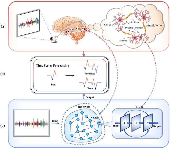
Figure 1. Proposed framework is based on the EICM neuron model of the mammalian visual cortex and uses it to construct a reservoir for performing time-series prediction tasks in chaotic systems.The EICM neuron model used in this framework is inspired by the dynamic characteristics of neurons in the mammalian primary visual cortex. Its core mechanism aims to more accurately simulate the real behavior of these biological neurons. By integrating the EICM neuron model (inspired by the V1 area of the primary visual cortex) into the reservoir, the constituent neurons are randomly interconnected via the weight matrix. (a)Visual pathway of the brain: Visual information from the retina is relayed via the lateral geniculate nucleus to the primary visual cortex (V1) and then processed in V2, V3, and V4, ultimately yielding patterns in the inferior temporal cortex. (b)Real vs. predicted time series. (c)ESN-EICM framework incorporates a V1 neuron model into reservoir computing to effectively forecast complex time-series sequences.

The remainder of this paper is organized as follows. Section 2 reviews related work in deep learning and reservoir computing for time series prediction. Section 3 details the proposed ESN-EICM model, including the EICM neuron design and the Bayesian optimization strategy. Section 4 describes the experimental setup and presents a thorough analysis of the results, covering prediction performance, hyperparameter sensitivity, and training time comparisons. Section 5 then discusses the broader implications of our findings, including the model’s design philosophy and its robustness against chaotic dynamics. Subsequently, Section 6 outlines the limitations of the current study and potential avenues for future research. Finally, Section 7 concludes the paper, summarizing the main contributions.

2 Related works

2.1 Deep learning-based time series prediction methods

With the continuous advancement of deep learning techniques, time series prediction has increasingly shifted toward neural network-based modeling strategies. The Recurrent Neural Network (RNN), proposed by Rumelhart et al. in 1986 [1], models sequential data through recurrent connections, effectively encoding historical information into hidden states. However, RNNs face challenges such as gradient vanishing and exploding gradients when handling long sequences, limiting their ability to capture long-term dependencies [2].

To address these limitations, Hochreiter and Schmidhuber introduced the Long Short-Term Memory (LSTM) network in 1997 [2]. LSTMs are specifically designed to retain long-range temporal information via sophisticated gating mechanisms (input, forget, and output gates), which control the flow of information through the cell. This architecture significantly improved the modeling of nonlinear data and has seen widespread application in diverse fields such as financial market prediction and climate modeling. Owing to their capacity to learn complex temporal dependencies and approximate highly nonlinear functions, LSTMs have also become a prominent benchmark for prediction chaotic time series, where accurately capturing long-range, intricate patterns is essential [13]. Indeed, studies have demonstrated LSTMs’ potential in predicting various chaotic systems, leveraging their ability to learn from historical data without explicit knowledge of the system’s underlying equations [14]. Nevertheless, despite their utility as a powerful baseline, the application of LSTMs, particularly to sensitive chaotic dynamics, is not without its difficulties. LSTM training demands substantial computational resources and a considerable amount of data to prevent overfitting, which can be a significant constraint in scenarios where data is scarce or computationally expensive to generate. They also exhibit high overall computational complexity [3], and their performance can be sensitive to hyperparameter choices, often requiring extensive tuning.

In contrast, the Gated Recurrent Unit (GRU) [3] simplifies the LSTM’s gating mechanism (employing update and reset gates) to reduce model complexity and the number of parameters. GRUs often demonstrate comparable or, in some cases, superior performance to LSTMs, especially in scenarios with limited data volume. However, they may still exhibit higher prediction errors when processing large-scale, highly complex datasets compared to more specialized architectures [4].

More recently, the Transformer architecture [4], originally developed for natural language processing, has transcended traditional recurrent networks through its self-attention mechanism. This allows for powerful parallel computation and has led to outstanding performance in large-scale sequence modeling tasks. However, the standard Transformer’s quadratic complexity with respect to sequence length and its potential sensitivity to noise in high-frequency or irregular time series can compromise its effectiveness for certain types of chaotic data without specific adaptations [15].

Despite ongoing methodological developments, deep learning models exhibit inherent limitations that are particularly pertinent to chaotic time series prediction: 1) Complex architectures generally lead to increased computational costs for training and inference. 2) Their “black-box” nature often weakens interpretability, hindering their deployment in domains requiring decision transparency or a deeper understanding of the model’s predictive reasoning (e.g., finance, healthcare, scientific discovery) [5]. For instance, while WaveNet [6] can model long sequences through dilated convolutions, it consumes excessive resources and is not easily parallelized. DeepAR [5], a probabilistic prediction model, may struggle with very sparse data scenarios sometimes encountered in chaotic systems. Furthermore, hybrid models like LSTM-FCN (LSTM Fully Convolutional Network) [16], while effective for classification, can face efficiency bottlenecks in feature fusion for regression tasks. Additionally, modifications aimed at reducing complexity in Transformers, such as the ProbSparse attention mechanism in the Informer model [15], can often discard critical subtle temporal patterns vital for chaotic systems, potentially degrading prediction stability. Beyond these established deep learning architectures, Spiking Neural Networks (SNNs), which more closely mimic biological neuronal dynamics through event-driven spike-based communication, are also being actively investigated for their potential in efficient temporal processing and learning, with research exploring aspects such as advanced training methodologies like adaptive smoothing gradient learning [17], effective parameter initialization techniques [18], and the role of noise [19]. SNNs are also finding applications in complex learning paradigms like brain-inspired reinforcement learning [20], and are also being developed for energy-efficient applications such as speech enhancement [21].

2.2 Reservoir computing for time series prediction

Diverging from deep learning approaches, Reservoir Computing (RC) offers novel insights through nonlinear dynamical systems. Echo State Networks (ESNs), introduced by Lukoševičius and Jaeger [7], map inputs into high-dimensional dynamic spaces via randomly connected reservoirs. Their efficiency stems from training only the output layer, yet performance critically depends on reservoir initialization and hyperparameter selection [7]. To overcome these limitations, researchers proposed innovations: Leaky ESN balances short-term dynamics and long-term memory through leakage parameters; Adaptive Elastic ESN optimizes reservoir weights using sparse Bayesian learning, dynamically adjusting sparsity to enhance multi-scale feature adaptation, though suffering from high training complexity and hyperparameter sensitivity [22]. Multi-reservoir ESN improves complex dynamic capture by parallelizing multiple reservoirs processing distinct frequency bands, but increases training complexity without unified state-fusion protocols. Deep Reservoir Computing [8] extracts hierarchical features via cascaded reservoirs, achieving excellence in long-period modeling while risking state inflation and overfitting. Recently, the SEP framework advanced lossless byte-stream prediction through semantic-enhanced compression [23], opening new directions for complex temporal modeling.

Current RC methods predominantly rely on simplistic neuron models, failing to simulate mammalian brain structures. This restricts generalization capabilities and robustness–simple reservoirs perform poorly on complex systems, while intricate designs induce overfitting and instability. Furthermore, although RC reduces RNN training costs, its fixed critical parameters necessitate manual tuning, lacking dynamic adaptability [7]. These constraints motivate the integration of biologically inspired neuron models (e.g., ICM) with reservoir computing, aiming to enhance chaos sequence prediction robustness through dynamic weight initialization strategies. The broader field of neuromorphic computing also explores various mechanisms for temporal processing in SNNs, including specialized modules designed to capture temporal shifts [24], build sequential memory [25], or adapt temporal characteristics [26].

3 Methods

3.1 Problem statement and challenges

The existing methods face the following challenges:

(1) The performance of reservoir computing models highly depends on critical hyperparameters such as reservoir size, spectral radius, and input scaling. These parameters not only influence dynamic characteristics (e.g., memory capacity and nonlinear mapping ability) but also directly determine prediction accuracy. In practical applications, extensive experiments and manual tuning are required to identify optimal parameter combinations, leading to significant time costs. Prediction errors vary widely under different configurations, particularly for high-dimensional and long-term sequences, where parameter sensitivity becomes more pronounced. Some parameter combinations even cause training divergence [27], [28].

(2) Most reservoir models rely on basic neuron designs that fail to simulate the complex connectivity and information-processing mechanisms of mammalian cortical neurons. While this simplification reduces implementation complexity, it limits expressive power for tasks involving long-term dependencies or abrupt feature detection. Traditional ESN models maintain reasonable accuracy in short-term predictions [29] but suffer rapid performance degradation with increasing sequence length and dynamic complexity. Model states decay over time, and sensitivity to abrupt changes diminishes [22].

(3) Although expanding reservoir size or introducing multi-layer structures can enhance model expressiveness and achieve low training errors, these modifications introduce new challenges. Increased complexity improves training fit but severely harms generalization on unseen data. Prediction errors fluctuate significantly during testing, indicating overfitting and poor robustness under noise or input distribution shifts. This highlights that boosting model complexity alone cannot resolve generalization issues in time series prediction [8].

3.2 Echo state network based on enhanced intersecting cortical model framework

3.2.1 Input layer

The input layer transforms raw time series data into feature representations suitable for subsequent processing. Given a time series input $u_t\in {\mathbb{R}}^D$, where $D$ denotes the input dimensionality, the input layer performs the following operation (Equation 1):

$S_t=W_{\text{in}}\cdot \left[1;u_t\right](1)$

where $[1;u_t]$ Adds a bias term to the input vector, and it allows the linear regression to learn an offset in the predictions in the output layers; $W_{in}\in {\mathbb{R}}^{N\times \left(D+1\right)}$ is input weight matrix, randomly initialized from a normal distribution, scaled by $input\text{\_}scale$, and subsequently its elements are clipped to the range $[-\mathrm{2,2}]$; $(N)$ is Reservoir size.

This approach ensures preliminary nonlinear mapping of input data while introducing an adjustable scaling factor $input\text{\_}scale$ to enhance adaptability to sequences with varying magnitudes [27].

3.2.2 Reservoir layer

The reservoir layer, the core component of ESN-EICM, comprises neurons governed by the Enhanced Intersecting Cortical Model (EICM). This design simulates biological feedback mechanisms and adaptive responses observed in mammalian cortical neurons.

The internal reservoir connectivity matrix $W\in {\mathbb{R}}^{N\times N}$ is constructed through the following steps:

• Elements of $W$ are drawn from a standard normal distribution and then multiplied by the scaling factor $w\text{\_}scale$.

•Sparsity is applied: a binary mask is generated where each element has a probability $w\text{\_}sparsity$ of being 1 (retaining the connection). The matrix $W$ is multiplied element-wise by this mask, effectively setting a fraction of connections to zero. Thus $w\text{\_}sparsity$ represents the desired connection density.

•The elements of the resulting sparse matrix are then clipped to the range [-1,1].

•Finally, the spectral radius of this processed matrix is normalized to the target $spectral\text{\_}radius$ value to help ensure Echo State Property and dynamic stability, as shown in Equation 2:

$W=W\cdot \left(\frac{\text{spectral\_radius}}{\max \left(|{\lambda }_i|\right)}\right)(2)$

The EICM neurons maintain internal states: $F$ (feeding input), $E$ (dynamic Threshold), and Y (Output term). Before the simulation begins (at time t = 0), these states are initialized. Specifically, $F$ and $E$ are initialized with random values drawn from a uniform distribution over [0, 0.1] and then their elements are clipped to the range [−1, 1]. The initial output states $Y$ are set to zeros. Each neuron updates its state using the following equations:

Each neuron updates its state using the EICM dynamics, which are detailed in Section 3.3.

•The feeding input $F_t$ is updated based on its prior value $F_{t=1}$, weighted feedback from other neurons in the reservoir $(W\cdot Y_{t=1})$, and the external stimulus $S_t$. This $F_t$ is then clipped.

•The neuron’s output $Y_t$ is generated using a Sigmoid activation function. The input to the sigmoid is the clipped difference between the current $F_t$ and the previous threshold $E_{t=1}$. Gaussian noise is added to the sigmoid’s output, and the final $Y_t$ is clipped to [0,1].

•The dynamic threshold $E_t$ adapts based on its previous value $E_{t=1}$ and the mean of the intermediate neuron activations before noise. This $E_t$ is also clipped.

For numerical stability, the primary state variables $F_t$ and $E_t$, as well as the difference term $F_t=E_{t=1}$, are clipped to the range [−50, 50] during their update.

The EICM neuron model introduces critical modifications to the original ICM framework [10]. Feeding input $F$ incorporates $W\cdot Y_{t-1}$ to enable cross-neuron interactions. This replaces the original ICM’s local dynamics $f$, $g$, $h$ with parameterized decay rates $f$, $g$, $h$. Threshold $E$ is updated using the population mean of $Y$, diverging from the original ICM’s local update rule. This prevents over-activation of individual neurons. Gaussian noise with standard deviation 0.001 is added to $Y$ for regularization and exploration enhancement. The exploitation of noise as a computational resource is also a recognized concept in other neuromorphic models such as SNNs [19]. After an initial period (of length initLen steps, where neuron states stabilize), the augmented state vectors are collected for training the output layer. Each augmented state vector is formed as $\mathrm{\Phi }(Y_t,u_t)=[1;u_t;Y_t]$, where $u_t$ is the external input vector at time $t$, $Y_t$ is the reservoir’s neuron output vector, and 1 represents a bias term. These augmented vectors form the columns of a matrix $X_{\mathit{collected}}=[\mathrm{\Phi }(Y_{\mathit{initLen}},u_{\mathit{initLen}}),\dots ,\mathrm{\Phi }(Y_T,u_T)]$. This $X_{\mathit{collected}}$ (referred to simply as X in the context of the output weight computation equation) is then used for training the output weights $W_{\mathit{out}}$.

3.2.3 Output layer

The output layer trains weights via regularized linear regression to produce predictions. Its equation is given by Equation 3:

${\widehat{y}}_t=W_{\text{out}}^{\top }\cdot \mathrm{\Phi }\left(Y_t,u_t\right)(3)$

where $\mathrm{\Phi }(Y_t,u_t)=[1;u_t;Y_t]$ represents the concatenated feature vector; $W_{\text{out}}\in {\mathbb{R}}^{(D+N+1)\times K}$ is output weight matrix, solved using Tikhonov-regularized least squares (Equation 4):

$W_{\text{out}}={\left(X{X}^{\top }+\lambda I\right)}^{-1}XY(4)$

where the regularization coefficient $\lambda \in [1e-\mathrm{8,1}e-2]$.

During inference, future states are recursively generated using historical inputs and reservoir states (Equation 5):

${\widehat{y}}_{t+1:T}=f\left(W_{\text{out}},\left\{u_t,Y_t\right\}\right)(5)$

3.2.4 Bayesian optimization strategy

To address the time-consuming manual hyperparameter tuning and susceptibility to local optima in traditional reservoir computing models, we introduce Bayesian Optimization (BO) within the ESN-EICM framework. BO constructs a surrogate function (e.g., Gaussian Process) and an acquisition function to efficiently balance exploration (sampling unexplored regions of the hyperparameter space) and exploitation (focusing on promising regions identified by prior evaluations). This approach rapidly converges to globally optimal configurations by leveraging information from prior experiments [30], a significant advancement over simpler strategies like grid or random search [31]. In our experiments, we employ the gp_minimize function (based on Gaussian Process Regression) for iterative parameter search. The optimization objective is defined as minimizing the mean squared error (MSE) on the validation set. To guide the optimization, the training data (the first 16,000 steps) was further partitioned: the first 14,000 steps were used to train the ESN-EICM’s output weights for a given hyperparameter set, and the subsequent 2,000 steps served as the validation set for calculating the MSE. The final reported test performance is evaluated on the held-out test set, which was never seen during training or optimization. Specify ranges and types (continuous/integers) for all parameters. Generate candidate hyperparameter combinations at each iteration and evaluate their MSE performance. Terminate the search process when the optimization objective (minimizing MSE) shows no significant improvement over consecutive iterations. Apply the optimal hyperparameter combination to train and test the final model. This strategy significantly reduces manual tuning costs while enhancing generalization capabilities for chaotic system prediction. The optimization space for ESN-EICM parameters is detailed in Table 1.

Table 1

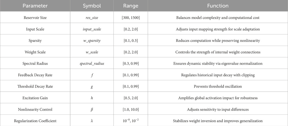
Table 1. ESN-EICM parameters optimization space.

3.3 Enhanced intersecting cortical model

The Enhanced Intersecting Cortical Model (EICM) neuron model (Figure 2 proposed in this work is built upon the original Intersecting Cortical Model (ICM) framework. The ICM was first introduced by Ekblad et al. [10], and was originally designed for image processing tasks—particularly for extracting features with indistinct boundaries. It simulates the behavioral characteristics of neurons in the mammalian primary visual cortex, including feedback mechanisms and adaptive threshold regulation.

Figure 2

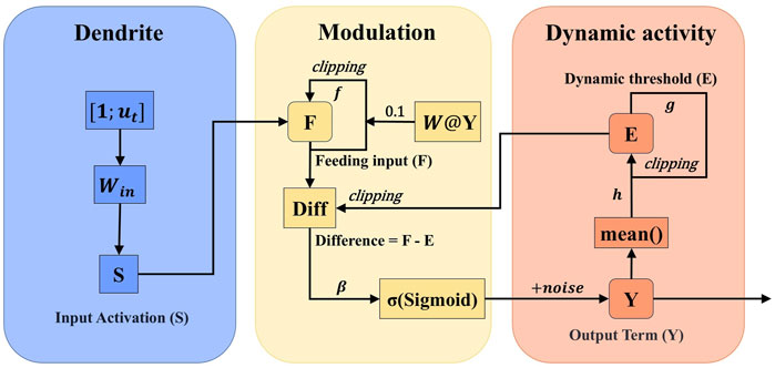
Figure 2. Enhanced Intersecting cortical model.

The original ICM neuron model consists of three key state variables: Feeding input $F$ is a feedback term representing historical input memory at the current time step; Dynamic threshold $E$ is an adaptive threshold that modulates neuron activation; Output term $Y$ is a binary output or activation state.

Its update equations are defined as follows (Equation 6):

$\left\{\begin{array}{cc}{F}_t\hfill & =f\cdot F_{t-1}+S_t\hfill \\ Y_t\hfill & =\left\{\begin{array}{cc}1,\hfill & \text{if}{F}_t>E_t\hfill \\ 0,\hfill & \text{otherwise}\hfill \end{array}\right.\hfill \\ E_t\hfill & =g\cdot E_{t-1}+h\cdot Y_t\hfill \end{array}\right.(6)$

where feedback decay rate $f$ controls the temporal decay of the feeding input; threshold decay rate $g$ Prevents threshold oscillation; Excitation gain $h$ regulates the strength of threshold updates based on neuron output; $S$ is External stimulus input; output term $Y$ equals 1 when the feeding input exceeds the dynamic threshold, and 0 otherwise.

This model has demonstrated strong edge detection and noise resistance capabilities in image segmentation applications. However, its binary output mechanism limits its expressiveness in time series modeling. Despite the biologically inspired structure and nonlinear mapping advantages of ICM, several critical limitations arise when applying it to time series prediction tasks such as chaotic system prediction:

(1) The model exhibits a lack of neuron-to-neuron coupling. The feeding input solely takes into account individual history and external input, without incorporating interactions across the reservoir.

(2) The local adaptation mechanism is limited as the dynamic threshold updates based merely on the current output of neuron, failing to reflect global network activity. The static parameter settings without range constraints also pose an issue, causing hyperparameters to remain fixed or loosely defined, which in turn leads to instability during training.

(3) The binary output limitation of the original ICM restricts its applicability to continuous-value regression tasks, as it only employs a binary pulse output of 0 or 1.

These issues significantly impair the ability of ICM to capture long-term dependencies and abrupt changes in complex nonlinear systems, resulting in suboptimal performance in chaotic time series modeling.

To enhance the modeling capability of the original ICM for time series prediction, we propose the EICM neuron design. The key improvements are outlined as follows:

(1) Improved sensitivity to long-range dependencies and abrupt changes. The original ICM model struggles with capturing long-term dependencies and detecting sudden signal transitions due to its local update mechanism. In EICM, we introduce global coupling through reservoir connectivity $(W\cdot Y_{t-1})$ and a mean-driven threshold adaptation strategy [32], enabling neurons to respond more sensitively to abrupt changes in chaotic systems [27].

(2) Enhanced Expressiveness for Continuous-Value Prediction. Unlike the binary pulse output in standard ICM, output term $Y$ EICM employs a continuous Sigmoid activation function. This modification allows the model to perform regression-based time series prediction tasks effectively, significantly expanding its applicability compared to the original image segmentation-oriented design.

(3) Integration of data-driven adaptation mechanisms. We redesign the dynamic threshold $E$ update rule by using the global mean activation of all neurons. This approach improves generalization and prevents local over-activation or under-activation, ensuring better consistency across the network during long-term prediction. This principle of integrating global network context to modulate local neuronal behavior is an active area of research, with concepts like context gating being explored in SNNs to achieve robust and adaptive learning, such as in lifelong learning scenarios [33].

(4) During the implementation, we imposed numerical range constraints on the parameters to enhance training stability, performed numerical clipping on $f$, $g$, $h$, $\beta$, and added Gaussian noise perturbations with a standard deviation of 0.001 after each activation to prevent overfitting and strengthen exploration capabilities.

These enhancements address the limitations of ICM in temporal modeling while preserving its biologically inspired structure. The EICM neuron model operates on three key state variables: the feeding input F, the dynamic threshold E, and the output term Y. To ensure a consistent starting point, these states are initialized at t = 0 as follows: $F$ and $E$ are populated with random values drawn from a uniform distribution $U(\mathrm{0,0.1})$, which are then clipped element-wise to the range [−1, 1]. This small, positive initialization range was chosen to ensure that neurons start in a responsive, non-saturated state, close to the linear region of the sigmoid activation function, which promotes stable initial dynamics as the reservoir settles. The update dynamics of the EICM neuron from time $t=1$ to $t$ proceed in the following equations (Equation 7):

$\left\{\begin{array}{cc}{F}_t\hfill & =f\cdot F_{t-1}+0.1\cdot \left(W\cdot Y_{t-1}\right)+S_t\hfill \\ Y_t\hfill & =\frac{1}{1+e^{-\beta \left(F_t-E_t\right)}}\hfill \\ E_t\hfill & =g\cdot E_{t-1}+h\cdot mean\left(Y_t\right)\hfill \end{array}\right.(7)$

These coupled dynamics allow the EICM neuron to maintain and process historical information over varying time scales, which is crucial for predicting chaotic systems. Effectively modeling such temporal dependencies is a key challenge in neural computation, with various architectures exploring mechanisms like dedicated delay units or gates to manage temporal information flow [34]. The core parameters intuitively govern the neuron’s behavior: $f$ (Feedback Decay Rate) controls the neuron’s short-term memory of its own past state; $g$ (Threshold Decay Rate) stabilizes the adaptive threshold, preventing overly rapid fluctuations; $h$ (Excitation Gain) determines how strongly the global network activity influences a neuron’s excitability; and $\beta$ (Nonlinearity Control) adjusts the steepness of the sigmoid activation, controlling the neuron’s sensitivity to the difference between its feeding input and its threshold. A higher $beta$ leads to a more switch-like, saturating behavior where the neuron’s output quickly approaches 0 or 1, while a lower $beta$ results in a smoother, more graded response across a wider range of inputs.

The enhanced performance of the ESN-EICM stems from the synergistic interaction between its two primary modifications: the global coupling feedback $(W\cdot Y_{t-1})$ and the global mean-driven adaptive threshold $(h\cdot \text{mean}(Y_t))$. These mechanisms work in concert to regulate the reservoir’s dynamics. The global coupling term ensures a rich and diverse set of inputs to each neuron, promoting complex, high-dimensional state representations and preventing the network from falling into simple, synchronized activity patterns. Concurrently, the adaptive threshold acts as a homeostatic, or self-regulating, mechanism. By adjusting each neuron’s excitability based on the average activity of the entire reservoir, it prevents runaway activation or quiescence. This homeostatic regulation keeps the reservoir in a critical “edge of chaos” regime, where it is most sensitive to input perturbations and possesses maximal memory capacity, which is crucial for stabilizing long-term predictions and effectively modeling chaotic dynamics.

3.3.1 Feeding input $F$

In the design of the feeding input $F$, we retain the exponential decay mechanism from the original ICM model, while introducing a dynamic coupling mechanism through the reservoir connectivity matrix $W$ to enable each neuron to perceive the overall state of the network. Where $F$ is first computed and then clipped to produce $F$. The coefficient 0.1 serves as a normalization factor for the reservoir feedback term. $S$ is the external driving stimulus. This enhancement significantly improves. The updated equation is defined as (Equation 8):

$F_t=f\cdot F_{t-1}+0.1\cdot \left(W\cdot Y_{t-1}\right)+S_t(8)$

where $f$ denotes the feedback decay rate, which controls the temporal decay of the historical feedback term and is constrained within a reasonable range to improve training stability; $W\cdot Y_{t-1}$ represents the influence from other neurons in the reservoir on the current neuron’s feedback input; The coefficient 0.1 serves as a normalization factor to prevent gradient explosion; $S$ is the external driving stimulus.

This enhancement significantly improves the suitability of the model for time series modeling by increasing inter-neuron information flow and cross-neuron coordination, thereby enhancing its nonlinear mapping capability compared to the original ICM framework.

3.3.2 Output term $Y$

To improve the expressiveness and robustness of the model, we replace the binary output mechanism in the original ICM with a multi-step process yielding a continuous output. First, the input to the sigmoid, $Delt{a}_t$, is calculated and clipped. The sigmoid function produces an intermediate output. Gaussian noise $\mathcal{N}(\mathrm{0,0.001})$ is then added, and finally, the output $Y$ is clipped to the range [0,1] to maintain stability and a consistent output scale. The updated output equation is given as (Equation 9):

$Y_t=\frac{1}{1+e^{-\beta \left(F_t-E_t\right)}}+\mathcal{N}\left(\mathrm{0,0.001}\right)(9)$

where $\beta$ controls the steepness of the activation function. The output values are no longer restricted to binary pulses (0 or 1), but instead fall within the continuous range [0,1] due to sigmoid activation and subsequent clipping. The standard deviation of 0.001 was chosen empirically as a value large enough to provide a regularizing effect and prevent overfitting, yet small enough not to disrupt the underlying learned dynamics of the system.

This improvement allows the model to more accurately capture subtle changes in input dynamics. The addition of small-scale noise injection further enhances exploration during training and improves generalization performance, particularly under noisy or uncertain conditions.

3.3.3 Dynamic threshold $E$

For the threshold update mechanism, we modify the original ICM approach which updates based on individual neuron output to a global mean-driven adaptation strategy. The updated equation is defined as (Equation 10):

$E_t=g\cdot E_{t-1}+h\cdot \text{mean}\left(Y_t\right)(10)$

where $g$ is the threshold decay rate that governs the temporal decay of the dynamic threshold; $h$ determines the gain factor of threshold adjustment; $\text{mean}(Y_t)$ represents the average activation across all neurons at time $t$.

This global adaptive thresholding strategy enables each neuron to adjust its response threshold according to the overall network activity, preventing certain neurons from being overly activated or suppressed. As a result, the model achieves greater stability and consistency across the reservoir.

4 Experiment

4.1 Dataset generation

To evaluate the predictive capabilities of the proposed ESN-EICM, ESN, and LSTM models, we generate three representative discrete chaotic system: Logistic system, Sine system, and Ricker system. These datasets are chosen for their distinct dynamic characteristics:

• Logistic System: A discrete-time chaotic system with strong nonlinearity.

•Sine System: A smooth periodic system with limited chaotic behavior.

•Ricker System: A biological population model exhibiting complex oscillatory patterns.

4.1.1 Data generation Process

Each dataset is generated using the following equations (Equations 11–13):

$\text{Logistic}\text{System:}{x}_{t+1}=3.8\cdot x_t\cdot \left(1-x_t\right)(11)$

$\text{Sine}\text{System:}{x}_{t+1}=0.9\cdot \sin \left(\pi x_t\right)(12)$

$\text{Ricker}\text{System:}{x}_{t+1}=x_t\cdot \exp \left(4\cdot \left(1-x_t\right)\right)\cdot 0.5(13)$

The initial value $x_0$ is set to $0.1$ for Logistic/Sine Maps and $0.5$ for Ricker Map. Each system is iterated for $T=20000$ steps. We then construct 3D feature vectors to capture nonlinear dependencies:

•Logistic System: $[x_t,x_t^2,x_t^3]$

•Sine System: $[x_t,\sin (x_t),\cos (x_t)]$

•Ricker System: $[x_t,\log (x_t+10^{-6}),\sqrt{x_t}]$

4.1.2 Data preprocessing

All datasets undergo the following preprocessing pipeline:

(1) Standardization: Data is standardized using Scikit-learn’s StandardScaler (Equation 14):

$x_{\text{scaled}}=\frac{x-\mu }{\sigma }(14)$

where $\mu$ and $\sigma$ are computed on the training split.

(2) Input-Target alignment: The input-output relationship is defined as (Equation 15):

$\text{inputs}={\mathbf{X}}_{1:T-1},\text{targets}={\mathbf{X}}_{2:T}(15)$

This ensures the model predicts $x_{t+1}$ given $x_t$.

(3) Train/Test Split: All systems use the same split (Equation 16):

$\text{trainLen}=16000,\text{testLen}=2000(16)$

The dataset was split chronologically to ensure strict temporal ordering and prevent information leakage from the test set into the training set. The first 16,000 steps were used for training and hyperparameter optimization, while the subsequent 2,000 steps were reserved exclusively for final testing. This partitioning is consistent across all systems to avoid introducing bias.

4.1.3 Dataset properties

A summary of the dataset configurations and properties is provided in Table 2.

Table 2

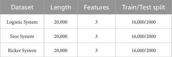
Table 2. Dataset configurations and properties.

4.2 Evaluation metrics

In our experiments, we compute the following evaluation metrics to quantify prediction performance. Let $y_i$ denote the ground truth value and ${\widehat{y}}_i$ the predicted value at time $i$, where $n=2000$ is the number of test samples.

4.2.1 Mean squared error (MSE)

The Mean Squared Error (MSE) measures the average squared difference between predicted and actual values. It’s a common metric for regression problems, penalizing larger errors more heavily. The equation is as follows (Equation 17):

$\text{MSE}=\frac{1}{n}{\displaystyle \sum _{i=1}^n}{\left(y_i-{\widehat{y}}_i\right)}^2(17)$

4.2.2 Root mean squared error (RMSE)

The Root Mean Squared Error (RMSE) is simply the square root of the MSE. It reflects the standard deviation of prediction errors and is in the same units as the target variable, making it more interpretable than MSE. The equation is as follows (Equation 18):

$\text{RMSE}=\sqrt{\text{MSE}}(18)$

4.2.3 Mean absolute error (MAE)

The Mean Absolute Error (MAE) measures the average absolute difference between predicted and actual values. Unlike MSE, MAE gives equal weight to all errors, making it more robust to outliers. The equation is as follows (Equation 19):

$\text{MAE}=\frac{1}{n}{\displaystyle \sum _{i=1}^n}|y_i-{\widehat{y}}_i|(19)$

4.2.4 Coefficient of determination $(R^2)$

The Coefficient of Determination $(R^2)$ quantifies the proportion of variance in the dependent variable that can be predicted from the independent variables. A value closer to 1 indicates that the model explains a larger proportion of the variance in the ground truth values. The equation is as follows (Equation 20):

$R^2=1-\frac{{\sum }_{i=1}^n{\left(y_i-{\widehat{y}}_i\right)}^2}{{\sum }_{i=1}^n{\left(y_i-\bar{y}\right)}^2}(20)$

4.2.5 Explained variance score (EVS)

The Explained Variance Score (EVS) evaluates how well the model captures the variance in the target variable. It’s similar to $R^2$ but can be more informative in cases where the model has a bias. The equation is as follows (Equation 21):

$\text{EVS}=1-\frac{\text{Var}\left(y_i-{\widehat{y}}_i\right)}{\text{Var}\left(y_i\right)}(21)$

4.2.6 Max error (ME)

The Max Error (ME) reports the maximum residual error between any predicted and actual value. This metric highlights the worst-case prediction scenario. The equation is as follows (Equation 22):

$\text{ME}=\underset{i=1,\dots ,n}{\max }|y_i-{\widehat{y}}_i|(22)$

4.3 Model configuration

This section details the configuration of the models employed in our comparative study: the proposed ESN-EICM, the baseline ESN, and the LSTM network. For the ESN-EICM and ESN models, hyperparameters were primarily determined through Bayesian Optimization, aiming to minimize Mean Squared Error on a validation set. For the LSTM model, key architectural and training hyperparameters were also optimized using Bayesian Optimization, while others were set based on common practices in time series forecasting. The specific search ranges and fixed values for each model are presented in the subsequent subsections. All models were trained and evaluated on the datasets described in Section 2 to ensure fair comparison.

4.3.1 ESN-EICM model configuration

Table 3 presents the key configuration parameters for the ESN-EICM model determined through Bayesian optimization in our experiments. A washout period initLen of 1000 steps was used for all experiments. This length was determined through preliminary observations to be sufficiently long to allow the reservoir’s internal state to become independent of its initial zero state and synchronize with the dynamics of the input signal across the range of tested hyperparameters.

Table 3

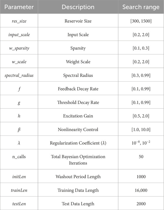
Table 3. ESN-EICM model Configuration parameters.

4.3.2 ESN model configuration

Table 4 presents the key configuration parameters for the Echo State Network (ESN) model determined through Bayesian optimization in our experiments.

Table 4

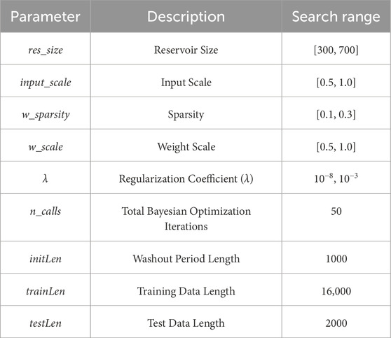
Table 4. ESN model Configuration parameters.

4.3.3 LSTM model configuration

Table 5 outlines the key configuration parameters for the Long Short-Term Memory (LSTM) network model. The hyperparameters were optimized using Bayesian optimization, while other parameters were set based on common practices.

Table 5

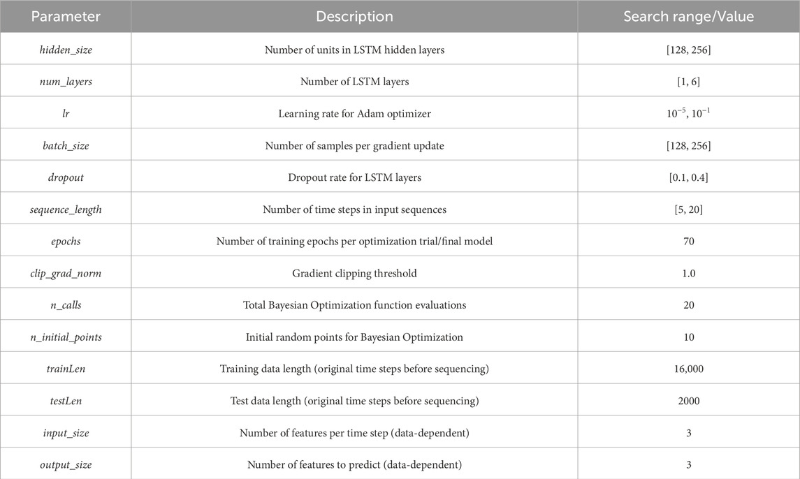
Table 5. LSTM model Configuration parameters.

4.4 Hyperparameter optimization results

To ensure optimal performance, critical hyperparameters for both the ESN-EICM and the baseline ESN models were determined using Bayesian Optimization. This process, guided by minimizing Mean Squared Error on a validation set as described in Section 3, yielded task-specific parameter configurations. The best-found parameters for each model across the different chaotic systems and prediction horizons are presented below.

4.4.1 ESN-EICM best parameters

The optimal hyperparameters identified for the proposed ESN-EICM model through Bayesian Optimization are summarized in Table 6. These parameters cover aspects of reservoir architecture, input processing, EICM neuron dynamics, and output regularization.

Table 6

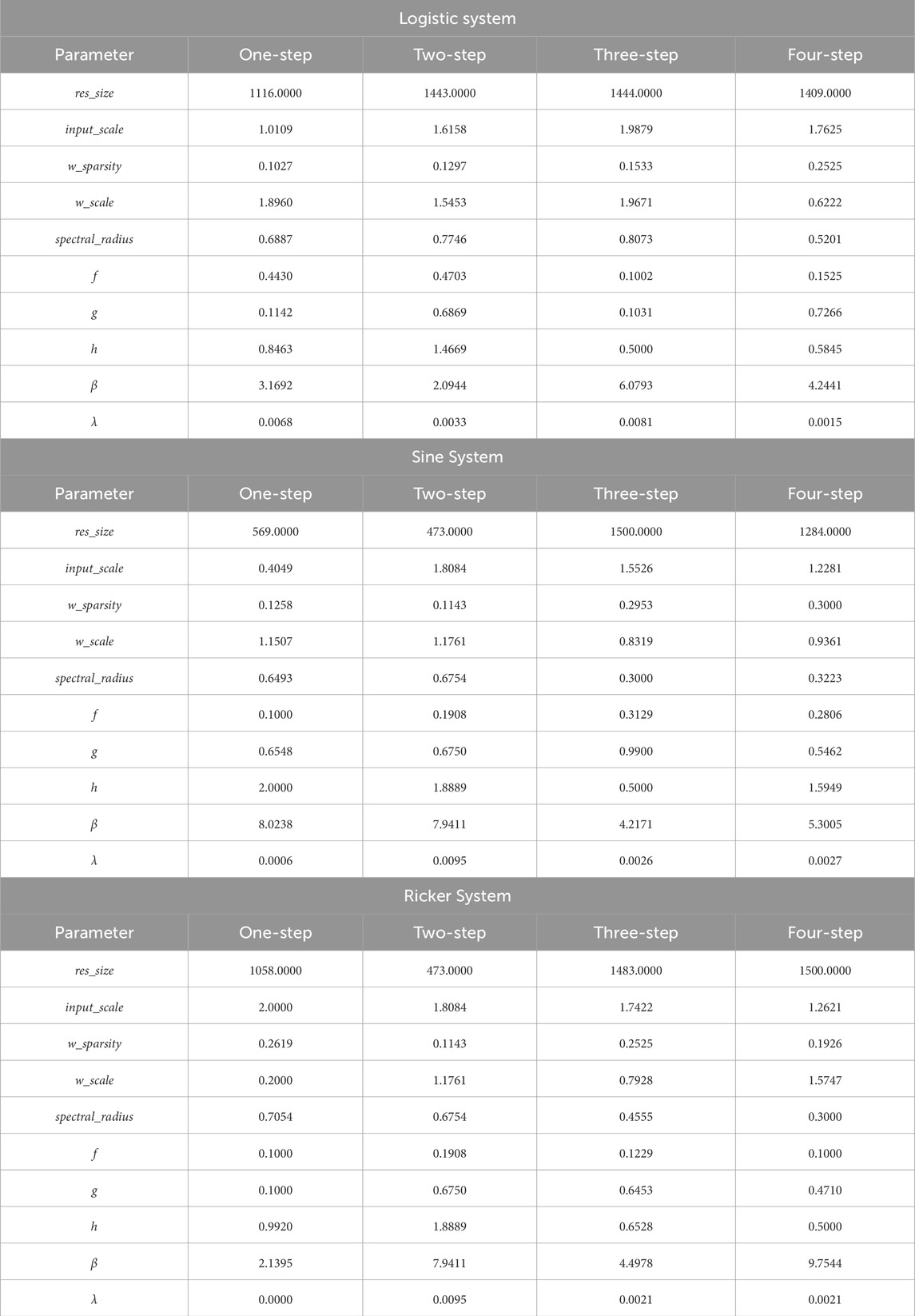
Table 6. Best ESN-EICM parameters for different chaotic systems and prediction steps.

4.4.2 ESN best parameters

For the baseline ESN model, the key hyperparameters tuned via Bayesian Optimization are detailed in Table 7. This allows for a direct comparison with the ESN-EICM model under similarly optimized conditions.

Table 7

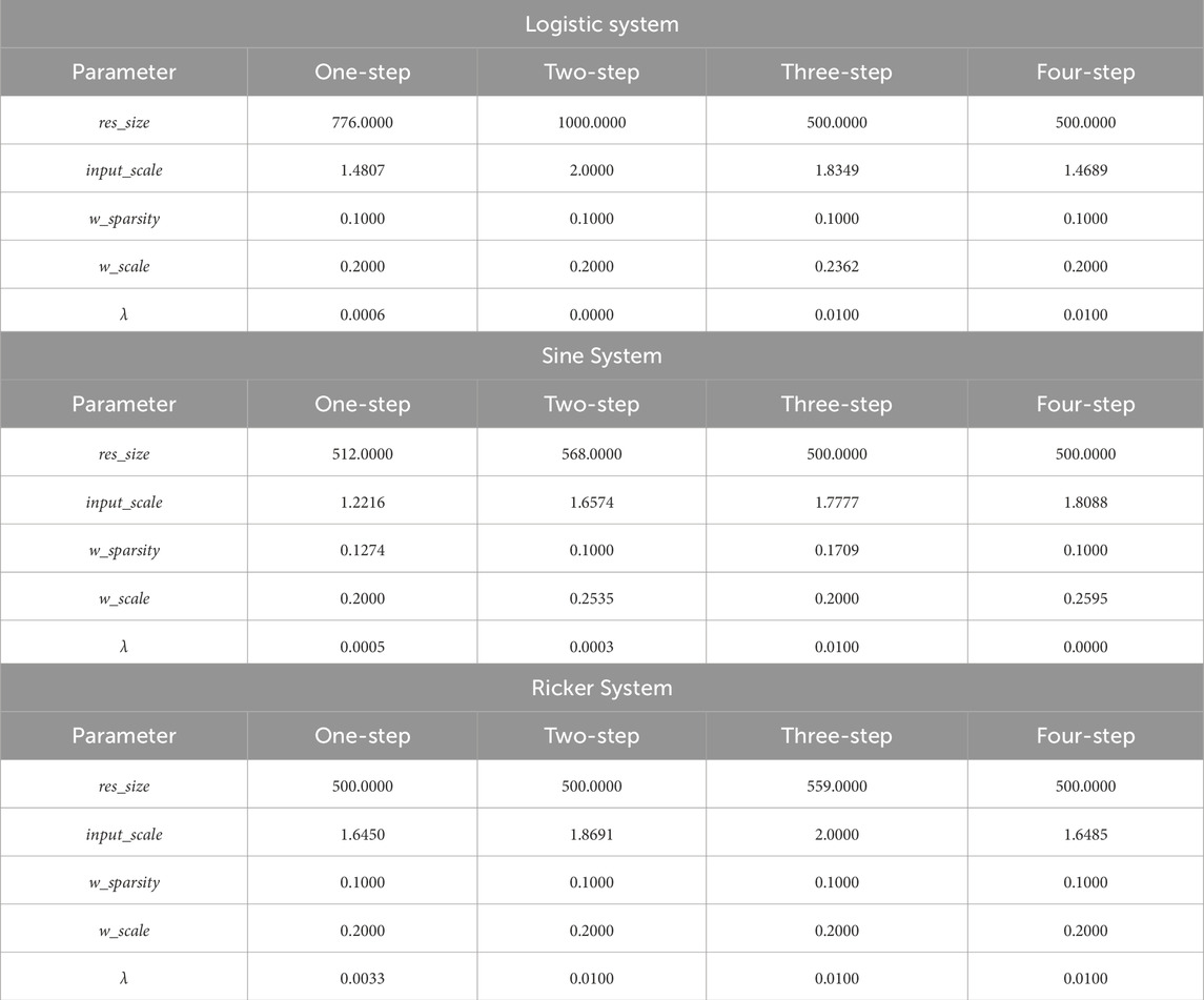
Table 7. Best ESN parameters for different chaotic systems and prediction steps.

4.4.3 LSTM best parameters

The Long Short-Term Memory (LSTM) network, serving as another important baseline, also underwent hyperparameter optimization using Bayesian Optimization. Key architectural and training parameters were tuned to achieve its best performance on each specific task. The optimized values for parameters such as hidden size, number of layers, learning rate, batch size, dropout rate, and input sequence length are presented in Table 8. These results reflect the optimal configurations found for the LSTM model across the different chaotic systems and prediction steps.

Table 8

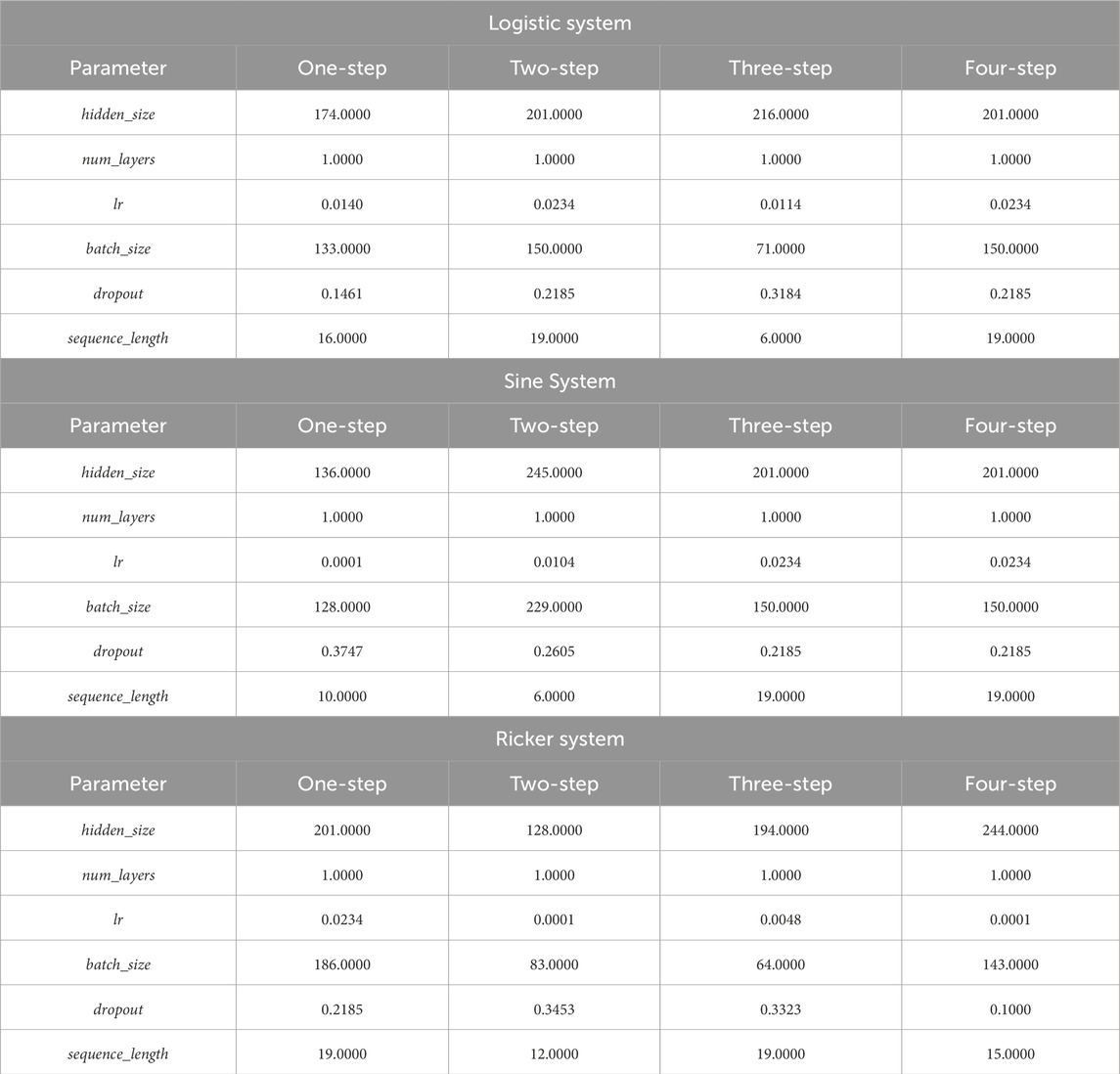
Table 8. Best LSTM parameters for different chaotic systems and prediction steps.

4.5 Hyperparameter sensitivity analysis

AS shown in Figure 3 (Logistic System), Figure 4 (Sine System), and Figure 5 (Ricker System), this section presents the hyperparameter sensitivity analysis for the ESN-EICM model. The analysis investigates the Mean Squared Error (MSE) response to variations in individual hyperparameters, while other parameters are held at their globally optimized values (from Table 6, for one-step prediction). This provides insights into each parameter’s influence on model performance and highlights the complexity of the hyperparameter landscape. The vertical dashed line in each plot marks the globally optimal value found by Bayesian Optimization.

Figure 3

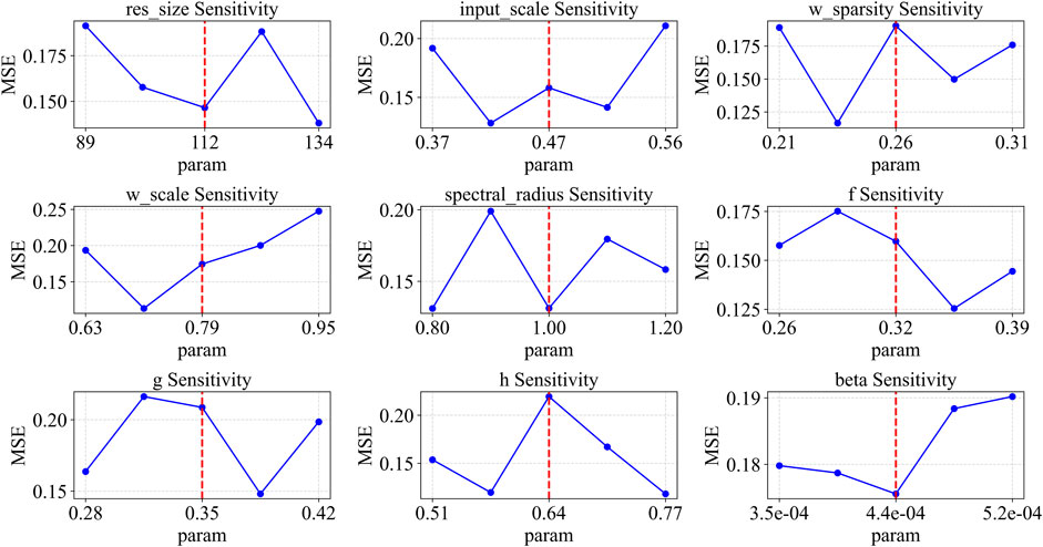
Figure 3. Parameter sensitivity analysis of ESN-EICM in logistic system.

Figure 4

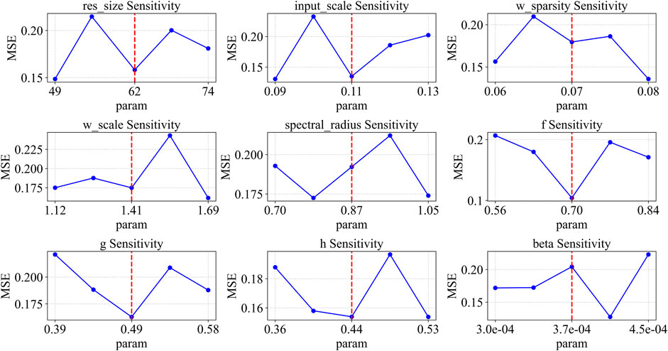
Figure 4. Parameter sensitivity analysis of ESN-EICM in sine system.

For the Logistic system, several parameters show high sensitivity. The res_size has a local minimum around the globally optimized value of 1116. Both input_scale and w_sparsity display V-shaped curves, with their local minima being slightly lower than their respective globally optimized values (marked at 1.01 and 0.10). The spectral_radius is critical, with its lowest MSE point aligning perfectly with the global optimum of 0.69. The EICM neuron parameters also show distinct patterns: f has a local minimum near 0.35, while its global optimum is 0.44. Both g and h exhibit U-shaped curves. Notably, beta is extremely sensitive, with its MSE sharply decreasing to a minimum that coincides with its global optimum of 3.17.

In the Sine system, the parameter sensitivities differ. res_size shows that larger reservoirs in the tested range yield better performance, with the global optimum at 569. For w_scale, a clear trend of decreasing MSE with smaller values is observed. Both spectral_radius and the neuron parameter f are highly sensitive, with sharp V-shaped curves where the local minima are very close to their global optima (0.65 and 0.10, respectively). The parameters g and h have broader optimal regions. For beta, the MSE is lowest at the higher end of the tested range, aligning with the global optimum of 8.02.

The Ricker system presents another unique sensitivity profile. Here, res_size has a relatively flat response curve, suggesting less sensitivity within this range compared to other systems. w_scale is highly critical, with a sharp V-shaped minimum. The spectral_radius plot shows that the global optimum of 0.71 is located on the slope of a broader minimum. For the EICM neuron parameters, f shows a preference for smaller values. The parameter h is highly sensitive, with a distinct local minimum. Finally, beta again demonstrates high sensitivity, with its local minimum near the globally optimized value of 2.14.

Across all three systems, parameters defining the EICM neuron’s core dynamics, such as f and beta, along with reservoir properties like spectral_radius and w_scale, consistently emerge as highly influential. Small deviations from their optimal values can lead to a significant increase in MSE, indicating that precise tuning of these parameters is crucial. In contrast, other parameters like res_size can exhibit broader optimal regions or system-dependent behaviors.

The analysis also reveals that the optimal hyperparameter configurations are distinct for each chaotic system, underscoring the necessity of system-specific optimization. While general trends can be observed, the precise values that minimize MSE vary considerably, highlighting the unique dynamic complexity of each system. This systematic analysis is fundamental for understanding the ESN-EICM’s behavior and validating the configurations found by our optimization strategy.

It is noteworthy that the optimal parameter values marked by the vertical dashed lines (representing the global optimum found by Bayesian Optimization) do not always coincide with the minimum MSE in each one-dimensional sensitivity plot. This is an expected and insightful result. Bayesian Optimization finds the best set of hyperparameters in a high-dimensional space where all parameters interact. In contrast, our sensitivity analysis examines one-dimensional slices of this space by varying a single parameter while keeping others fixed at their global optimal values. The discrepancy between the global optimum and the local minima in these plots highlights the strong coupling and interdependencies among the hyperparameters. It demonstrates that the ideal value for one parameter is contingent on the values of others, reinforcing the necessity of using a multi-dimensional optimization strategy like Bayesian Optimization rather than relying on one-at-a-time parameter tuning.

4.6 Prediction performance evaluation

4.6.1 One-step prediction performance

The efficacy of the ESN-EICM model for one-step prediction was rigorously evaluated on three canonical chaotic systems: the Logistic system, the Sine system, and the Ricker system. Its performance was benchmarked against both traditional ESN and LSTM architectures. The comprehensive results, encompassing both quantitative metrics and qualitative visualizations, consistently underscore the superior predictive accuracy and robustness of the proposed ESN-EICM.

Quantitative analysis, detailed in Table 9, reveals that ESN-EICM generally achieves lower error metrics compared to ESN and LSTM. For instance, in predicting the Logistic system, ESN-EICM recorded a MSE of $5.3281\times 10^{-8}$ and a RMSE of $2.3083\times 10^{-4}$. This trend of superior accuracy was also observed for the Sine system, with ESN-EICM yielding an MSE of $2.5966\times 10^{-8}$ and an RMSE of $1.6114\times 10^{-4}$. These figures are notably lower than those of the benchmark models, indicating a more precise alignment between ESN-EICM’s predictions and the ground truth. Even for the Ricker system, the MSE of ESN-EICM of $1.9910\times 10^{-7}$ demonstrated a substantial improvement over the traditional ESN $(4.2969\times 10^{-6})$. Furthermore, ESN-EICM exhibited competitive MAE values across all systems, achieving the lowest MAE for the Sine map $(7.6498\times 10^{-5})$ and demonstrating MAEs comparable to or better than ESN and LSTM for the Logistic and Ricker system. While all models displayed high R² and Explained Variance scores, ESN-EICM distinguished itself by coupling this high explanatory power with consistently lower prediction errors and well-contained Maximum Errors, as seen for the Logistic $(6.6633\times 10^{-3})$ and Sine system $(5.3483\times 10^{-3})$, highlighting its predictive stability.

Table 9

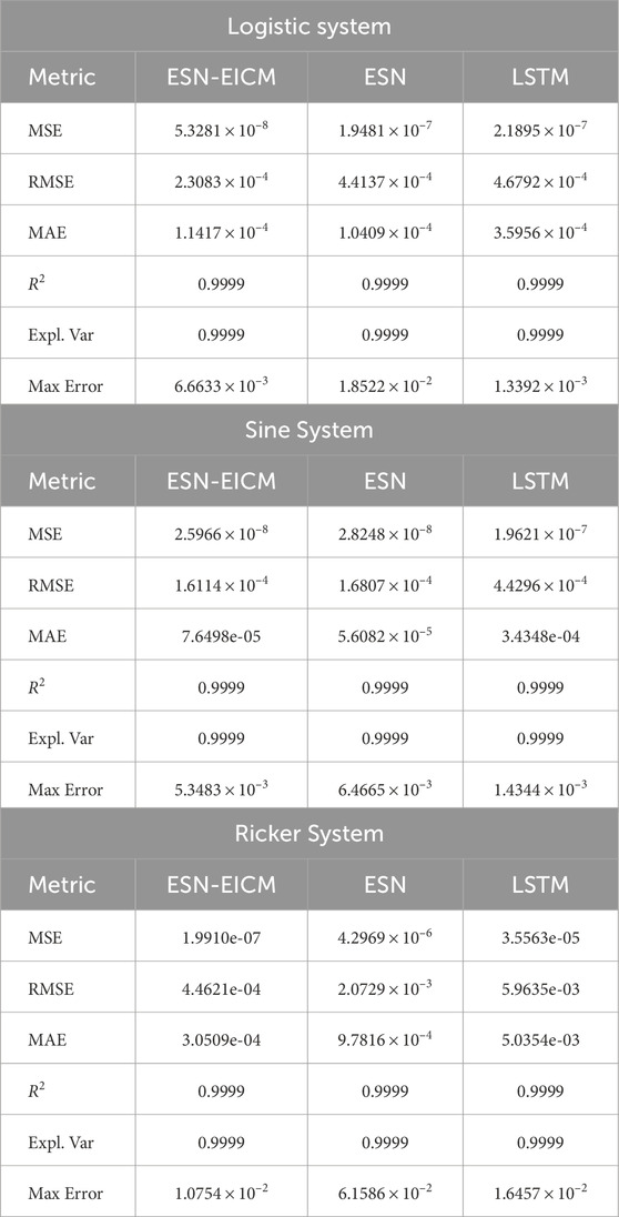
Table 9. One-step prediction performance by different chaotic system.

The qualitative visualizations further reinforce these quantitative findings. The one-step prediction trajectories, illustrated in Figure 6 (assuming this figure shows predicted vs. true time series plots), demonstrate the ESN-EICM’s capability to closely track the actual system dynamics for the Logistic system (a), Sine map (b), and Ricker model (c), even through complex behavioral regimes. The temporal evolution of absolute prediction error, as depicted in Figure 7, confirms the stability of ESN-EICM’s predictions, with errors remaining at consistently low levels (typically on the order of $10^{-3}$ or less) without significant accumulation or divergence for all three systems. Moreover, the phase space reconstructions presented in Figure 8 show a remarkable congruence between the attractors generated from ESN-EICM’s predictions (red markers) and those of the true systems (blue markers). The model accurately reproduces the characteristic geometries of Logistic map’s phase space plot (a), the Sine map’s phase space plot (b), and the Ricker model’s phase space plot (c), indicating to its proficiency in capturing the underlying nonlinear dynamics. Finally, the scatter plots in Figure 9, which compare predicted values against true values, show data points tightly clustered around the ideal $y=x$ diagonal for all systems (a, b, c). This high degree of linearity and consistency provides direct visual evidence of ESN-EICM’s superior predictive precision.

Figure 5

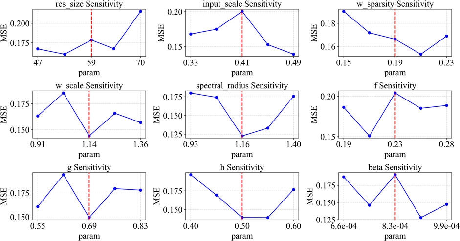
Figure 5. Parameter sensitivity analysis of ESN-EICM in ricker system.

Figure 6

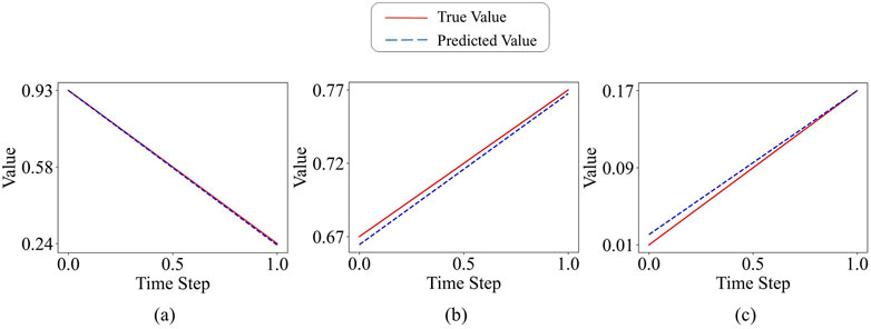
Figure 6. ESN-EICM One-step Prediction in Different Chaotic Systems: (a) the Logistic system, (b) the Sine system, and (c) the Ricker system.

Figure 7

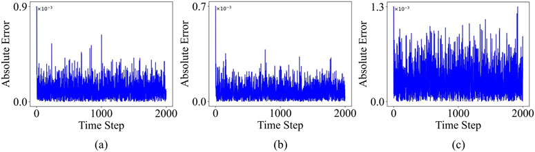
Figure 7. ESN-EICM One-step Prediction Absolute Error Over Time in Different Chaotic Systems: (a) the Logistic system, (b) the Sine system, and (c) the Ricker system.

Figure 8

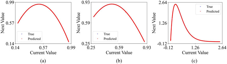
Figure 8. ESN-EICM One-step Prediction Phase Space Reconstruction in Different Chaotic Systems: (a) the Logistic system, (b) the Sine system, and (c) the Ricker system.

Figure 9

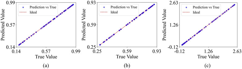
Figure 9. ESN-EICM One-step Prediction Accuracy: Predicted vs. True Values in Different Chaotic Systems: (a) the Logistic system, (b) the Sine system, and (c) the Ricker system.

In conclusion, the combined evidence from quantitative metrics and qualitative visualizations strongly supports the enhanced performance of the ESN-EICM model in one-step prediction tasks for chaotic time series. It consistently outperforms or matches established models like ESN and LSTM in accuracy and robustness, while also demonstrating a strong capability to learn and replicate the intricate dynamics inherent in these complex systems. These results firmly establish ESN-EICM as a promising and effective tool for nonlinear time series prediction.

4.6.2 Multi-step prediction performance

To further assess the predictive capabilities of the proposed ESN-EICM model, comprehensive multi-step prediction experiments were conducted for two-step, three-step, and four-step ahead forecasts. These predictions were performed on the Logistic, Sine, and Ricker chaotic systems, and the performance of ESN-EICM was benchmarked against standard ESN and LSTM models. The quantitative results for these multi-step predictions are detailed in Table 10 (two-step), Table 11 (three-step), and Table 12 (four-step). Visualizations of the ESN-EICM’s multi-step prediction trajectories, corresponding absolute errors, phase space reconstructions, and scatter plots of predicted versus true values are presented in Figures 10–13, respectively.

Table 10

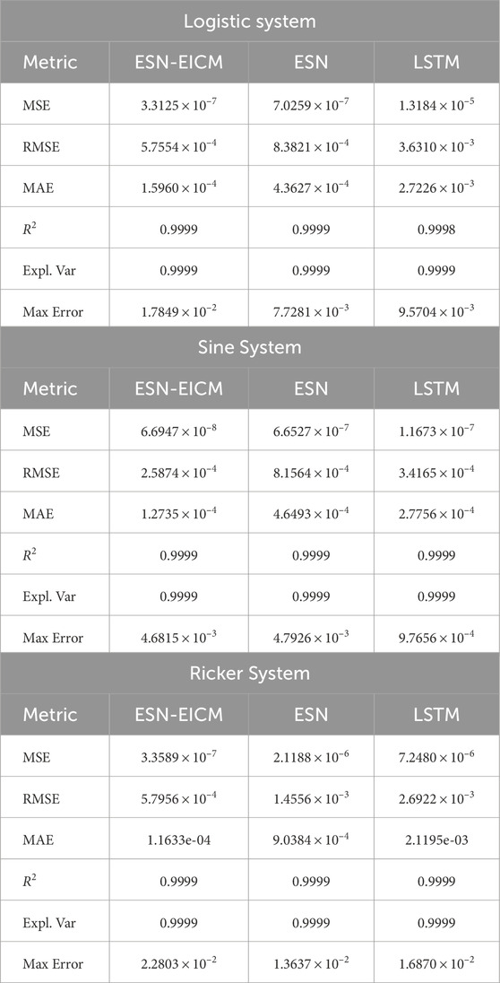
Table 10. Two-step prediction performance metrics by different chaotic systems.

Table 11

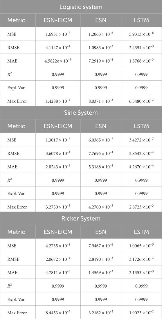
Table 11. Three-step prediction performance metrics by different chaotic systems.

Table 12

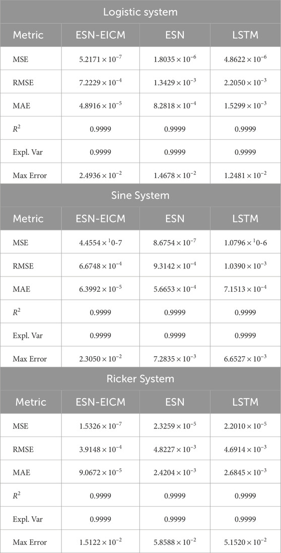
Table 12. Four-step prediction performance metrics by different chaotic systems.

Figure 10

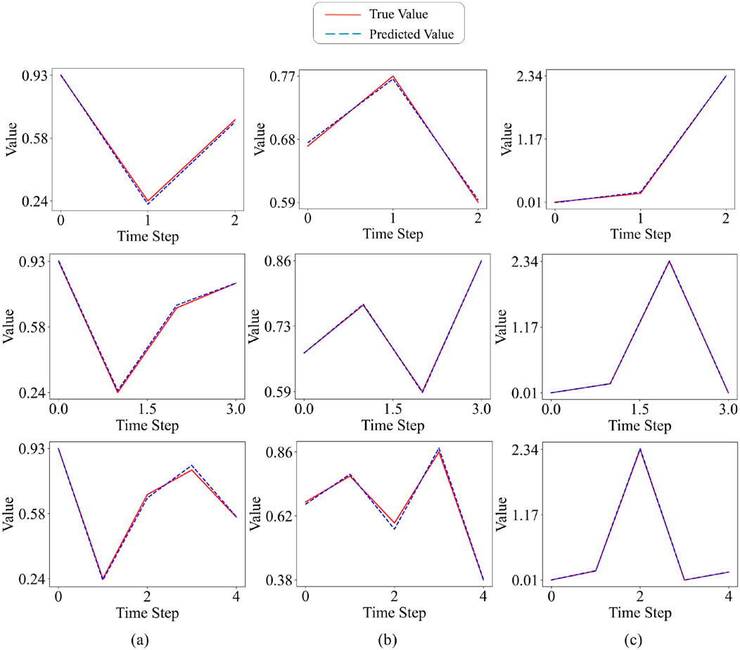
Figure 10. ESN-EICM multi-step Prediction in Different Chaotic Systems: (a) the Logistic system, (b) the Sine system, and (c) the Ricker system.

Figure 11

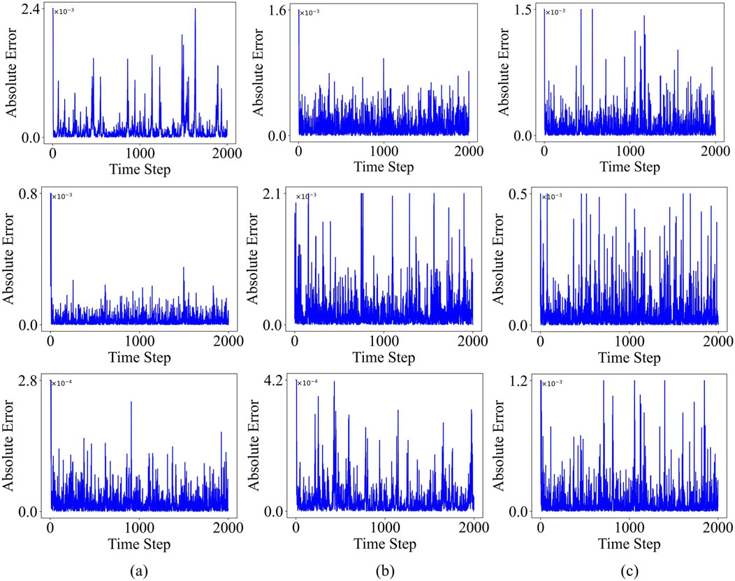
Figure 11. ESN-EICM multi-step Prediction Absolute Error Over Time in Different Chaotic Systems: (a) the Logistic system, (b) the Sine system, and (c) the Ricker system.

Figure 12

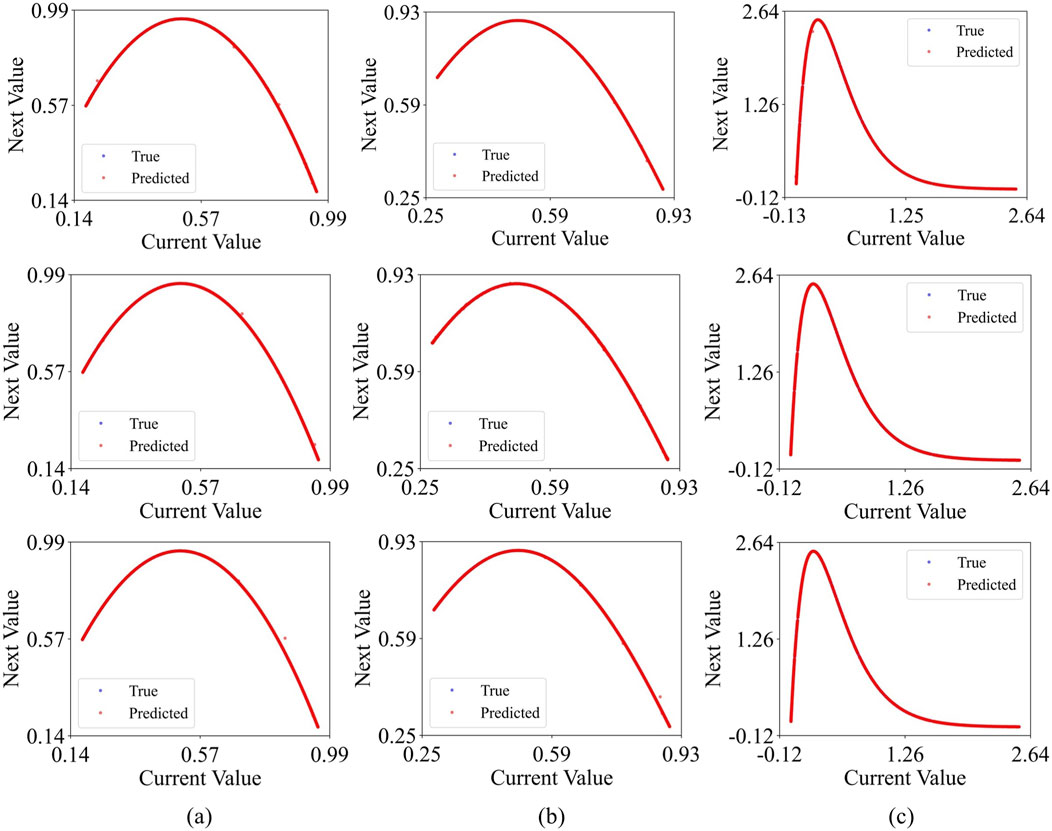
Figure 12. ESN-EICM multi-step Prediction Phase Space Reconstruction in Different Chaotic Systems: (a) the Logistic system, (b) the Sine system, and (c) the Ricker system.

Figure 13

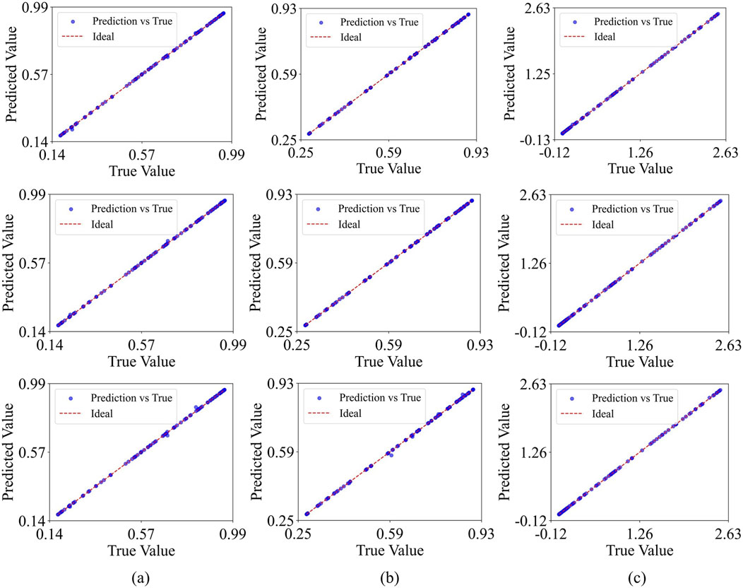
Figure 13. ESN-EICM multi-step Prediction Accuracy: Predicted vs. True Values in Different Chaotic Systems: (a) the Logistic system, (b) the Sine system, and (c) the Ricker system.

Visually, Figures 10–13 collectively demonstrate the robust performance of the ESN-EICM model in multi-step prediction. Figure 10 shows that the predicted trajectories for all three chaotic systems ((a) Logistic, (b) Sine, (c) Ricker) closely follow the true system dynamics even over extended horizons. The absolute errors, as depicted in Figure 11, remain consistently low and bounded over the 2000 time steps, indicating the stability and accuracy of the ESN-EICM. The fidelity of the model in capturing the underlying dynamics of these chaotic systems is further highlighted by the phase space reconstructions in Figure 12, where the predicted attractors exhibit excellent agreement with the true attractors. Moreover, the scatter plots in Figure 13 show data points tightly clustered around the ideal diagonal line (Predicted Value = True Value), underscoring the high point-wise accuracy of the ESN-EICM in multi-step prediction scenarios.

Quantitatively, the ESN-EICM model consistently outperforms both ESN and LSTM across nearly all metrics and prediction horizons for the three chaotic systems.

For the Logistic system, in 2-step predictions (Table 10), ESN-EICM achieved an MSE of $3.3125\times 10^{-7}$, markedly lower than ESN $(7.0259\times 10^{-7})$ and LSTM $(1.3184\times 10^{-5})$. This superiority in terms of MSE, RMSE, and MAE was maintained and often accentuated as the prediction horizon increased. For instance, in 4-step predictions (Table 12), ESN-EICM’s MSE was $5.2171\times 10^{-7}$ and MAE was $4.8916\times 10^{-5}$, significantly better than ESN (MSE: $1.8035\times 10^{-6}$, MAE: $8.2818\times 10^{-4}$) and LSTM (MSE: $4.8622\times 10^{-6}$, MAE: $1.5299\times 10^{-3}$).

In the case of the Sine system, ESN-EICM also demonstrated consistently lower MSE, RMSE, and MAE. For 2-step predictions (Table 10), ESN-EICM’s MSE $(6.6947\times 10^{-8})$ was superior to both ESN $(6.6527\times 10^{-7})$ and LSTM $(1.1673\times 10^{-7})$. While LSTM occasionally yielded a lower Max Error (e.g., $9.7656\times 10^{-4}$ for 2-steps), ESN-EICM’s average error metrics remained dominant. This trend persisted for 4-step predictions (Table 12), where ESN-EICM’s MAE of $6.3992\times 10^{-5}$ was substantially lower than ESN’s $5.6653\times 10^{-4}$ and LSTM’s $7.1513\times 10^{-4}$.

The Ricker system results particularly highlight the strength of the ESN-EICM. For 2-step predictions (Table 10), ESN-EICM’s MSE $(3.3589\times 10^{-7})$ was already an order of magnitude better than LSTM $(7.2480\times 10^{-6})$ and significantly better than ESN $(2.1188\times 10^{-6})$. This advantage became even more pronounced at longer horizons. For 3-step predictions (Table 11), ESN-EICM achieved an exceptionally low MSE of $4.2735\times 10^{-8}$, two orders of magnitude smaller than ESN $(7.9467\times 10^{-6})$ and LSTM $(1.0065\times 10^{-5})$. It also recorded the lowest Max Error $(8.4453\times 10^{-3})$ in this scenario. This pattern continued for 4-step predictions (Table 12), where ESN-EICM’s MSE $(1.5326\times 10^{-7})$ and Max Error $(1.5122\times 10^{-2})$ were notably superior to the comparator models.

Across all tested scenarios, R² and Explained Variance values were consistently close to 0.9999 for all models, indicating a good general fit. However, the significant differences in MSE, RMSE, and MAE clearly underscore the enhanced precision and robustness of the ESN-EICM model for multi-step chaotic time series prediction. The sustained low error levels, even as the prediction horizon extends, suggest that ESN-EICM effectively captures the complex underlying dynamics and is less prone to error accumulation compared to standard ESN and LSTM approaches in these multi-step prediction tasks.

4.7 Training time comparison

In this section, we describe the measurement of the execution times of the three models for the same prediction task. The computer configuration is as follows:

• RAM: 32.0 GB (31.2 GB available)

•Processor: AMD Ryzen 9 7945HX with Radeon Graphics, 2.50 GHz

•System: 64-bit operating system, x64-based processor

•Operating System: Windows 11 Pro, version 24H2

•Graphics Card: NVIDIA GeForce RTX 4060 Laptop GPU, 8 GB GPU VRAM, NVIDIA

•Python: 3.12.0

•NumPy version: 1.26.4

•SciPy version: 1.14.1

•scikit-learn version: 1.5.2

•Matplotlib version: 3.9.2

•scikit-optimize version: 0.10.2

•tqdm version: 4.66.5

•torch version: 2.7.0

•Pandas version: 2.2.3

The computational efficiency of the proposed ESN-EICM model was evaluated against traditional ESN and LSTM architectures, with total experiment times recorded in Table 13. A key advantage of reservoir computing models, including ESN and our ESN-EICM, lies in their training efficiency compared to deep learning models like LSTM. This is primarily because the reservoir’s internal weights are fixed after initialization, and only the output weights are trained, typically through a computationally inexpensive linear regression. In contrast, LSTMs require iterative backpropagation through time and gradient descent over many epochs (70 epochs in our setup, as per 4.3.3), leading to significantly longer training durations. This fundamental difference is evident across all prediction steps and chaotic systems, where both ESN-EICM and ESN consistently outperform LSTM in terms of speed, often by an order of magnitude. For instance, in one-step prediction for the Logistic system, ESN-EICM took 424.3 s, ESN took 398.8 s, while LSTM required 1649.0 s. This pattern persists and often magnifies in multi-step scenarios; for example, in four-step prediction for the Ricker system, ESN-EICM completed in 570.5 s, ESN in 4006.0 s, and LSTM in 2092.1 s.

Table 13

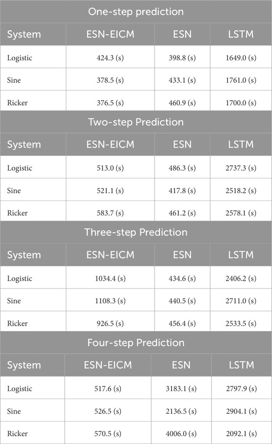
Table 13. Total experiment time for different prediction steps, chaotic systems, and models.

When comparing ESN-EICM specifically with the standard ESN, the time performance presents a nuanced but ultimately favorable picture for ESN-EICM, particularly as prediction horizons extend. In one-step and two-step predictions, the ESN-EICM’s runtime is generally comparable to that of the standard ESN, occasionally slightly higher. This marginal increase can be attributed to the more complex neuron dynamics within the ESN-EICM reservoir (as described in Section 3), which involve updates for feeding input $F$, output $Y$ with sigmoid activation and noise, and a dynamic threshold $E$ based on mean population activity. These richer per-neuron computations, while enhancing predictive power, incur a slight overhead per time step during reservoir state generation compared to the simpler activation function of a traditional ESN.

However, a significant advantage for ESN-EICM emerges in longer multi-step predictions, particularly at the four-step horizon. Here, ESN-EICM demonstrates substantially better time efficiency than the standard ESN. For example, in four-step prediction for the Logistic system, ESN-EICM took only 517.6 s, whereas ESN’s time escalated to 3183.1 s. Similar substantial speed-ups for ESN-EICM over ESN were observed for the Sine (526.5 s vs. 2136.5 s) and Ricker (570.5 s vs. 4006.0 s) systems at four steps. This pronounced improvement in efficiency for ESN-EICM in more challenging, longer-term prediction tasks can be directly attributed to how its enhanced stability impacts the Bayesian Optimization process. The inherent stability of the EICM neurons—stemming from features like adaptive thresholds and bounded activations—creates a “smoother” hyperparameter landscape for the optimizer to explore. This means that fewer parameter combinations lead to divergent or numerically unstable models, which would otherwise result in extremely high error values (penalties) and waste optimization calls. For the standard ESN, finding a stable parameter set for long-term iterative prediction can be more difficult, leading the optimizer to spend more time evaluating poorly performing or unstable regions. In contrast, the ESN-EICM’s robustness means that a larger proportion of the hyperparameter space yields valid, stable models, allowing the Bayesian optimizer to more quickly identify near-optimal configurations in fewer iterations. Therefore, the “faster convergence” mentioned in the abstract is not about the speed of a single training run, but the efficiency of the entire hyperparameter search process, which is significantly accelerated by the model’s intrinsic stability.

5 Discussion

5.1 On model complexity and the design philosophy

A central tenet of traditional ESNs is the use of a simple, fixed reservoir to reduce training complexity. Our ESN-EICM model, by incorporating a more complex neuron, appears to diverge from this principle. This is a deliberate design choice motivated by the specific challenge of chaotic system prediction. Instead of seeking complexity through architectural modifications like deep or multi-reservoir structures, we pursue “internal complexification” at the neuronal level. The rationale is that the rich, adaptive dynamics of the EICM neuron—with its coupled feedback and adaptive thresholds—can generate a more expressive variety of temporal patterns. This allows a reservoir of a given size to map the input into a higher-quality, more dynamically rich state space. The performance gains observed, particularly in multi-step prediction, suggest that for highly complex and sensitive systems like the ones studied, the benefits of enhanced neuronal dynamics outweigh the modest increase in per-neuron computational cost. This approach offers a valuable alternative to topological optimization, focusing instead on the intrinsic computational capabilities of the reservoir’s constituent elements.

5.2 Robustness against sensitivity in chaotic systems

The introduction mentions the “butterfly effect,” the extreme sensitivity of chaotic systems to initial conditions. The ESN-EICM’s strong performance in multi-step prediction suggests an inherent robustness against this sensitivity. This can be attributed to several design features. The adaptive threshold mechanism $(E_t)$ acts to normalize the network’s overall activity, preventing small initial errors from being catastrophically amplified and causing state divergence. The internal feedback $(f\cdot F_{t-1})$ and global coupling $(W\cdot Y_{t-1})$ create a rich, stable attractor dynamic within the reservoir that is resistant to minor perturbations. Finally, the injection of a small amount of noise can be seen as a form of regularization that prevents the model from overfitting to a specific trajectory, thereby improving its ability to generalize and remain on the true system’s attractor for longer during iterative prediction.

6 Limitations and future work

While the proposed ESN-EICM model has demonstrated significant advantages in prediction chaotic time series, certain limitations and avenues for future research warrant discussion.

6.1 Limitations

1. Although Bayesian Optimization (BO) is more efficient than grid search or random search, optimizing a relatively large number of hyperparameters (10 in this study for ESN-EICM, as shown in Table 1) can still be computationally intensive, especially if each evaluation (training and validating the model) is time-consuming due to large reservoir sizes or long time series. The 50 calls to BO used in this study represent a trade-off between search thoroughness and computational budget.

2. The computational complexity of standard ESN training involves matrix operations that scale with reservoir size $(N)$. While the EICM neuron introduces a constant factor overhead per neuron, the fundamental scaling properties of RC remain. For extremely large reservoirs, the memory and computational demands for storing and operating on the reservoir weight matrix $W$ and collecting states could become a bottleneck.

3. The ESN-EICM was evaluated on three discrete chaotic systems, which are well-defined and exhibit specific types of chaos. Real-world time series often contain multiple sources of noise, non-stationarities, and varying types of underlying dynamics that were not explicitly addressed or modeled in this study beyond the inherent learning capacity of the reservoir. The model’s performance on such diverse and potentially more complex real-world datasets remains to be extensively validated.

4. While the EICM neuron model is biologically inspired and its mechanisms (adaptive threshold, feedback) are more transparent than the internal workings of an LSTM cell, the collective dynamics of a large reservoir of interconnected EICM neurons can still be complex to analyze and interpret fully. Understanding precisely how the EICM parameters $(f,g,h,\beta )$ contribute to specific dynamic properties like memory capacity or nonlinearity at the network level requires further investigation.

5. The EICM neuron parameters $(f,g,h,\beta )$ are optimized via BO and then fixed during training and inference. For highly non-stationary time series, dynamically adapting these internal neuron parameters online could potentially offer further performance improvements.

6. While the overall training is efficient, the EICM neuron itself is computationally more demanding than a standard tanh or sigmoid neuron due to the multiple state updates (F, E, Y) required at each time step. This introduces a constant factor overhead in the reservoir state generation phase, which could become noticeable for very large reservoirs or extremely long time series.

6.2 Future work

Based on the promising results and current limitations, several directions for future research can be pursued:

1. Exploring more sophisticated or parallelized Bayesian optimization techniques, or meta-learning approaches to warm-start BO, could further reduce the hyperparameter tuning cost. Investigating gradient-based optimization for certain EICM parameters, if feasible, might also be an avenue.

2. Developing mechanisms for online adaptation of key EICM parameters $(f,g,h,\beta )$ based on the input statistics or prediction error could enhance the model’s adaptability to changing dynamics in non-stationary environments.

3. Combining ESN-EICM with other machine learning techniques could yield synergistic benefits. For example, using attention mechanisms in the output layer or employing ESN-EICM as a feature extractor for a subsequent shallow neural network could be explored.

4. A more in-depth theoretical analysis of the ESN-EICM, focusing on its memory capacity, echo state property conditions with EICM neurons, and stability criteria, would provide a stronger foundational understanding.

5. Extending the application of ESN-EICM to a wider range of challenging real-world chaotic and complex time series from domains such as finance (stock market prediction), climate science (weather prediction), engineering (system identification), and neuroscience (EEG signal analysis) would be crucial for demonstrating its practical utility.

6. Investigating the integration of other sophisticated, biologically plausible neuron models (e.g., Izhikevich neurons, adaptive exponential integrate-and-fire models) within the RC framework could lead to further advancements in time series prediction.Further exploration into neuromorphic hardware implementations could also be beneficial, drawing insights from ongoing research into memristive systems and their complex dynamics for specialized tasks [35]. Similarly, advancements in cellular neural networks coupled with novel devices like memristors also contribute to the broader landscape of hardware-oriented neural computation [36]. Exploring efficient hardware avenues, such as FPGA implementations for complex and novel neural architectures, remains an important direction [37].

7. Beyond hyperparameter optimization, exploring techniques for optimizing the reservoir’s topology (e.g., using pruning or growing methods guided by EICM neuron activity) could lead to more efficient and specialized reservoir structures.

Addressing these limitations and exploring these future research directions will contribute to advancing the field of reservoir computing and its application to complex time series analysis.

7 Conclusion

In this work, we introduced the Echo State Network Based on Enhanced Intersecting Cortical Model (ESN-EICM), a novel reservoir computing framework designed for accurate and efficient prediction of dicrete chaotic systems. Recognizing the limitations of traditional deep learning models in terms of computational cost and interpretability, and the constraints of standard ESNs concerning simplistic neuron dynamics and hyperparameter sensitivity, the ESN-EICM offers a compelling alternative. The core innovation lies in the integration of biologically inspired EICM neurons into the reservoir, characterized by continuous sigmoid activation, global mean-driven adaptive thresholds, and explicit inter-neuron feedback. This design endows the reservoir with richer internal dynamics, better suited for capturing the complex patterns inherent in chaotic systems. Furthermore, the adoption of a Bayesian Optimization strategy systematically addresses the challenge of hyperparameter tuning, leading to robust and near-optimal model configurations.

Our comprehensive experimental evaluation on the Logistic, Sine, and Ricker chaotic systems unequivocally demonstrated the ESN-EICM’s superiority. In both one-step and challenging multi-step prediction tasks (up to four steps ahead), the ESN-EICM consistently outperformed both standard ESN and LSTM models, as evidenced by significantly lower Mean Squared Error, Root Mean Squared Error, and Mean Absolute Error. Qualitative analyses, including prediction trajectory plots, error distributions, phase space reconstructions, and scatter plots, further visually corroborated the enhanced accuracy and stability of the ESN-EICM. Notably, while maintaining the characteristic training efficiency of RC models over LSTMs, the ESN-EICM often exhibited comparable or even superior total experiment times (including optimization) compared to standard ESNs in multi-step scenarios, attributed to the increased stability and expressiveness of the EICM neurons facilitating a more efficient hyperparameter search.

The successful application of EICM neurons within an ESN framework, coupled with automated hyperparameter optimization, highlights the potential of integrating more sophisticated, biologically plausible mechanisms into reservoir computing. The ESN-EICM stands as a robust, accurate, and computationally viable tool for modeling and predicting chaotic time series, paving the way for further research into neuro-inspired computing paradigms for complex dynamical systems. Future work will focus on extending its application to diverse real-world problems, exploring dynamic adaptation of neuron parameters, and conducting further theoretical analysis of its properties.

Data availability statement

The original contributions presented in the study are included in the article/supplementary material, further inquiries can be directed to the corresponding author.

Author contributions

XW: Conceptualization, Writing – review and editing, Writing – original draft, Visualization, Project administration, Data curation, Methodology. PM: Resources, Conceptualization, Funding acquisition, Writing – review and editing, Writing – original draft, Validation, Software. JnL: Resources, Investigation, Writing – original draft, Funding acquisition, Writing – review and editing, Data curation, Project administration, Supervision. JzL: Project administration, Funding acquisition, Supervision, Writing – review and editing, Writing – original draft, Data curation, Resources, Validation. YM: Resources, Funding acquisition, Formal Analysis, Writing – review and editing, Project administration, Supervision, Conceptualization, Writing – original draft, Data curation.

Funding

The author(s) declare that financial support was received for the research and/or publication of this article. Some experiments are supported by the Supercomputing Center of Lanzhou University. Additionasupport was provided in part by the Gansu Computing Center.

Conflict of interest

The authors declare that the research was conducted in the absence of any commercial or financial relationships that could be construed as a potential conflict of interest.

Generative AI statement

The author(s) declare that no Generative AI was used in the creation of this manuscript.

Publisher’s note

All claims expressed in this article are solely those of the authors and do not necessarily represent those of their affiliated organizations, or those of the publisher, the editors and the reviewers. Any product that may be evaluated in this article, or claim that may be made by its manufacturer, is not guaranteed or endorsed by the publisher.

References

1. Rumelhart DE, Hinton GE, Williams RJ. Learning representations by back-propagating errors. nature (1986) 323:533–6. doi:10.1038/323533a0

CrossRef Full Text | Google Scholar

2. Hochreiter S, Schmidhuber J. Long short-term memory. Neural Comput (1997) 9:1735–80. doi:10.1162/neco.1997.9.8.1735

PubMed Abstract | CrossRef Full Text | Google Scholar

3. Chung J, Gulcehre C, Cho K, Bengio Y. Empirical evaluation of gated recurrent neural networks on sequence modeling. arXiv preprint arXiv:1412.3555 (2014). doi:10.48550/arXiv.1412.3555

CrossRef Full Text | Google Scholar

4. Vaswani A, Shazeer N, Parmar N, Uszkoreit J, Jones L, Gomez AN, et al. Attention is all you need. Adv Neural Inf Process Syst (2017) 30. doi:10.48550/arXiv.1706.03762

CrossRef Full Text | Google Scholar

5. Salinas D, Flunkert V, Gasthaus J, Januschowski T. Deepar: probabilistic forecasting with autoregressive recurrent networks. Int J Forecast (2020) 36:1181–91. doi:10.1016/j.ijforecast.2019.07.001

CrossRef Full Text | Google Scholar

6. Van Den Oord A, Dieleman S, Zen H, Simonyan K, Vinyals O, Graves A, et al. Wavenet: a generative model for raw audio. arXiv preprint arXiv:1609.03499 12 (2016). doi:10.48550/arXiv.1609.03499

CrossRef Full Text | Google Scholar

7. Lukoševičius M, Jaeger H. Reservoir computing approaches to recurrent neural network training. Computer Sci Rev (2009) 3:127–49. doi:10.1016/j.cosrev.2009.03.005

CrossRef Full Text | Google Scholar

8. Gallicchio C, Micheli A, Pedrelli L. Deep reservoir computing: a critical experimental analysis. Neurocomputing (2017) 268:87–99. doi:10.1016/j.neucom.2016.12.089

CrossRef Full Text | Google Scholar

9. He L, Xu Y, He W, Lin Y, Tian Y, Wu Y, et al. Network model with internal complexity bridges artificial intelligence and neuroscience. Nat Comput Sci (2024) 4:584–99. doi:10.1038/s43588-024-00674-9

PubMed Abstract | CrossRef Full Text | Google Scholar

10. Ekblad U, Kinser JM, Atmer J, Zetterlund N. The intersecting cortical model in image processing. Nucl Instr Methods Phys Res Section A: Acc Spectrometers, Detectors Associated Equipment (2004) 525:392–6. doi:10.1016/j.nima.2004.03.102

CrossRef Full Text | Google Scholar

11. Tang Y, Jia S, Huang T, Yu Z, Liu JK. Implementing feature binding through dendritic networks of a single neuron. Neural Networks (2025) 189:107555. doi:10.1016/j.neunet.2025.107555

PubMed Abstract | CrossRef Full Text | Google Scholar

12. Zheng H, Zheng Z, Hu R, Xiao B, Wu Y, Yu F, et al. Temporal dendritic heterogeneity incorporated with spiking neural networks for learning multi-timescale dynamics. Nat Commun (2024) 15:277. doi:10.1038/s41467-023-44614-z

PubMed Abstract | CrossRef Full Text | Google Scholar

13. Shi X, Chen Z, Wang H, Yeung D-Y, Wong W-K, Woo W-C., et al. Convolutional lstm network: a machine learning approach for precipitation nowcasting. Adv Neural Inf Process Syst (2015) 28. doi:10.48550/arXiv.1506.04214

CrossRef Full Text | Google Scholar

14. Awad M. Forecasting of chaotic time series using rbf neural networks optimized by genetic algorithms. Int Arab J Inf Technology (Iajit) (2017) 14.

Google Scholar

15. Zhou H, Zhang S, Peng J, Zhang S, Li J, Xiong H, et al. Informer: beyond efficient transformer for long sequence time-series forecasting. Proc AAAI Conf Artif intelligence (2021) 35:11106–15. doi:10.1609/aaai.v35i12.17325

CrossRef Full Text | Google Scholar

16. Karim F, Majumdar S, Darabi H, Chen S. Lstm fully convolutional networks for time series classification. IEEE access (2017) 6:1662–9. doi:10.1109/access.2017.2779939

CrossRef Full Text | Google Scholar

17. Wang Z, Jiang R, Lian S, Yan R, Tang H. Adaptive smoothing gradient learning for spiking neural networks. In: International conference on machine learning. New York, NY, USA: Proceedings of Machine Learning Research (2023). p. 35798–816.

Google Scholar

18. Ding J, Zhang J, Huang T, Liu JK, Yu Z. Assisting training of deep spiking neural networks with parameter initialization. IEEE Trans Neural Networks Learn Syst (2025) 1–14. doi:10.1109/tnnls.2025.3547774

PubMed Abstract | CrossRef Full Text | Google Scholar

19. Ma G, Yan R, Tang H. Exploiting noise as a resource for computation and learning in spiking neural networks. Patterns (2023) 4:100831. doi:10.1016/j.patter.2023.100831

PubMed Abstract | CrossRef Full Text | Google Scholar

20. Yang Z, Guo S, Fang Y, Yu Z, Liu JK. Spiking variational policy gradient for brain inspired reinforcement learning. IEEE Trans Pattern Anal Machine Intelligence (2024) 47:1975–90. doi:10.1109/tpami.2024.3511936

PubMed Abstract | CrossRef Full Text | Google Scholar

21. Hao X, Ma C, Yang Q, Wu J, Tan KC. Toward ultralow-power neuromorphic speech enhancement with spiking-fullsubnet. IEEE Trans Neural Networks Learn Syst (2025) 1–15. doi:10.1109/tnnls.2025.3566021

PubMed Abstract | CrossRef Full Text | Google Scholar

22. Xu M, Han M. Adaptive elastic echo state network for multivariate time series prediction. IEEE Trans cybernetics (2016) 46:2173–83. doi:10.1109/tcyb.2015.2467167

PubMed Abstract | CrossRef Full Text | Google Scholar

23. Qin Z, Tao X, Lu J, Tong W, Li GY. Semantic communications: principles and challenges. arXiv preprint arXiv:2201.01389 (2021). doi:10.48550/arXiv.2201.01389

CrossRef Full Text | Google Scholar

24. Yu K, Zhang T, Xu Q, Pan G, Wang H. Ts-snn: temporal shift module for spiking neural networks. arXiv preprint arXiv:2505.04165 (2025).

Google Scholar

25. Zhang M, Luo X, Wu J, Belatreche A, Cai S, Yang Y, et al. Toward building human-like sequential memory using brain-inspired spiking neural models. IEEE Trans Neural Networks Learn Syst (2025) 36:10143–55. doi:10.1109/tnnls.2025.3543673

PubMed Abstract | CrossRef Full Text | Google Scholar

26. Zhang J, Zhang M, Wang Y, Liu Q, Yin B, Li H, et al. Spiking neural networks with adaptive membrane time constant for event-based tracking. IEEE Trans Image Process (2025) 34:1009–21. doi:10.1109/tip.2025.3533213

PubMed Abstract | CrossRef Full Text | Google Scholar

27. Lian J, Yang Z, Liu J, Sun W, Zheng L, Du X, et al. An overview of image segmentation based on pulse-coupled neural network. Arch Comput Methods Eng (2021) 28:387–403. doi:10.1007/s11831-019-09381-5

CrossRef Full Text | Google Scholar

28. Lukoševičius M. A practical guide to applying echo state networks. In: Neural networks: tricks of the trade. 2nd ed. Springer (2012). p. 659–86.

Google Scholar

29. Jaeger H, Haas H. Harnessing nonlinearity: predicting chaotic systems and saving energy in wireless communication. science (2004) 304:78–80. doi:10.1126/science.1091277

PubMed Abstract | CrossRef Full Text | Google Scholar

30. Snoek J, Larochelle H, Adams RP. Practical bayesian optimization of machine learning algorithms. Adv Neural Inf Process Syst (2012) 25. doi:10.48550/arXiv.1206.2944

CrossRef Full Text | Google Scholar

31. Bergstra J, Bengio Y. Random search for hyper-parameter optimization. J machine Learn Res (2012) 13:281–305.

Google Scholar

32. Carandini M, Heeger DJ. Normalization as a canonical neural computation. Nat Rev Neurosci (2012) 13:51–62. doi:10.1038/nrn3136

PubMed Abstract | CrossRef Full Text | Google Scholar

33. Shen J, Ni W, Xu Q, Pan G, Tang H. Context gating in spiking neural networks: achieving lifelong learning through integration of local and global plasticity. Knowledge-Based Syst (2025) 311:112999. doi:10.1016/j.knosys.2025.112999

CrossRef Full Text | Google Scholar

34. Sun P, Wu J, Zhang M, Devos P, Botteldooren D. Delayed memory unit: modeling temporal dependency through delay gate. IEEE Trans Neural Networks Learn Syst (2024) 36:10808–18. doi:10.1109/tnnls.2024.3490833

PubMed Abstract | CrossRef Full Text | Google Scholar

35. Yu F, He S, Yao W, Cai S, Xu Q. Quantitative characterization system for macroecosystem attributes and states. IEEE Trans Computer-Aided Des Integrated Circuits Syst (2025) 36:1–12. doi:10.13287/j.1001-9332.202501.031

PubMed Abstract | CrossRef Full Text | Google Scholar

36. Yu F, Su D, He S, Wu Y, Zhang S, Yin H. Resonant tunneling diode cellular neural network with memristor coupling and its application in police forensic digital image protection. Chin Phys B (2025) 34:050502. doi:10.1088/1674-1056/adb8bb

CrossRef Full Text | Google Scholar

37. Yu F, Zhang S, Su D, Wu Y, Gracia YM, Yin H. Dynamic analysis and implementation of fpga for a new 4d fractional-order memristive hopfield neural network. Fractal and Fractional (2025) 9:115. doi:10.3390/fractalfract9020115

CrossRef Full Text | Google Scholar