Optimizing dynamic pull-in threshold and periodic trajectories for magnetically actuated MEMS (magMEMS) in wearable sensors

Magnetically actuated micro-electro-mechanical systems (magMEMSs) are pivotal for wearable sensor applications that need high sensitivity, fast response, and compact integration, such as biomedical monitoring and motion-tracking devices. In this paper, we investigate the dynamic pull-in instability and periodic trajectory analysis of magMEMS models with current-carrying filaments, addressing critical challenges in a miniaturized sensor design. A simplified Galerkin approach is used to analyze a Lorentz-force-driven MEMS oscillator, deriving approximate expressions for the dynamic pull-in threshold—a key criterion for stable periodic operation—and the corresponding oscillation frequency and periodic solutions. Extensive numerical simulations support and validate the analytical results. These findings offer valuable insights to assist in the design and optimization of MEMS devices in wearable sensors.

1 Introduction

Micro-electro-mechanical systems (MEMSs) have revolutionized numerous fields by enabling the development of miniaturized devices with exceptional performance and diverse functionalities, particularly in wearable sensor technologies where compactness, low power consumption, and high sensitivity are paramount. These systems combine mechanical, electrical, and optical components in a single device of micrometric dimensions, forming compact, multifunctional chips when integrated with electronic signal-processing units [1, 2]. In wearable applications—such as biomedical monitoring (e.g., real-time health tracking via magnetoencephalography probes), environmental sensing, and motion-tracking systems—MEMSs offer unparalleled advantages, including their ability to detect minute physical changes (e.g., magnetic field fluctuations and mechanical vibrations) with fast response times [3, 4]. Characterized by their compact size and energy efficiency, MEMSs are ideal for power-constrained wearable devices operating in the Internet of Things (IoT) ecosystem [5, 6]. Among MEMS subclasses, magnetically actuated MEMSs (magMEMSs) have emerged as a promising solution for wearable sensors due to their linear response, directional actuation, and dimensional stability at the nanoscale [7, 8], making them suitable for applications requiring precise, repeatable displacement control in dynamic environments (e.g., wearable accelerometers or flexible biosensors).

However, a major challenge in the performance and reliability of magMEMSs is pull-in instability—a nonlinear phenomenon that can significantly impair device operation. This instability occurs when the magnetic attraction between a movable microstructure (such as a beam, plate, or membrane) and a magnetic actuator (typically a coil or permanent magnet) exceeds the mechanical restoring force. Beyond a critical threshold—referred to as the pull-in point—the structure collapses onto the actuator, often irreversibly, leading to permanent device failure [9–13].

This behavior is particularly problematic in magMEMS actuators and sensors, where precise and repeatable displacement control is crucial. The issue becomes even more critical in nanoelectromechanical systems (NEMSs), which utilize components typically smaller than 100 nm. At such scales, proximity forces—including Van der Waals forces, covalent bonding, and electrostatic interactions—can dominate over the magnetic driving force, adding further complexity to the dynamics [14, 15]. The strong nonlinear interaction between magnetic forces and structural elasticity is typically modeled through coupled magneto-mechanical equations [16], posing substantial challenges for both theoretical analysis and practical design. A rigorous investigation of pull-in dynamics under magnetostatic loading is thus essential for ensuring robust and safe operation of magMEMS devices.

To address this challenge, a variety of analytical, numerical, and semi-analytical methods have been developed. The variational iteration method (VIM) is widely appreciated for its flexibility in handling nonlinear dynamics [17, 18]; however, its practical application is often hindered by the difficulty in constructing appropriate Lagrange multipliers. Alternatives include reduced-order modeling, phase-plane analysis, and perturbation methods, which aim to approximate the pull-in threshold and capture critical behavior near instability points [9, 19, 20]. Energy-based methods and bifurcation analysis offer qualitative insights into collapse dynamics [11], whereas numerical continuation and shooting methods allow for high-accuracy tracking of periodic orbits and stability boundaries [10]. Semi-analytical frameworks such as the homotopy perturbation method (HPM) are also popular [21] although they are sensitive to initial guesses and homotopy construction. To enhance convergence and reliability, hybrid methods combining homotopy with Laplace transforms have been proposed [22].

Di Barba et al. [23] developed a geometric formulation of the electrostatic field in membrane MEMS devices, in which the electric field magnitude is assumed to be proportional to the membrane curvature. Although focused on electrostatic actuation, this work shares strong methodological parallels with the present study. This parallel is particularly evident in the treatment of singular nonlinearities and instability conditions, for which rigorous existence results were established using Schauder–Tychonoff’s fixed-point theorem. In fact, the analytical insights from the electrostatic framework by Di Barba et al. [23], especially those concerning solution existence and uniqueness, also provide a mathematical foundation for the magnetodynamic model developed here. Additionally, frequency-based approximations have been explored by reformulating the problem into a standard form amenable to harmonic solutions [24–26]. Recently, there has been a resurgence of interest in classical analytical techniques, which often yield surprisingly accurate results with minimal computational effort [27, 28]. Frequency-based methods, while conceptually simple and non-iterative, may sacrifice some accuracy in capturing complex dynamics [29]. Algebraic techniques leveraging Sturm’s theorem have also shown promise as fast and reliable tools for approximating pull-in thresholds [30, 31].

In this context, the present work makes a novel contribution to the analysis of magMEMS by studying a Lorentz-force-driven model involving current-carrying filaments using a simple and effective Galerkin approximation. Unlike transformation-based techniques required for harmonic approximations under zero initial conditions [24], our method yields closed-form expressions for the dynamic pull-in threshold, oscillation frequency, and periodic trajectories. In particular, we derive an explicit pull-in condition that serves as a practical criterion for the existence of periodic orbits. The analytical results are systematically validated through numerical simulations, confirming their accuracy across a broad range of parameters. This approach enhances the understanding of nonlinear dynamics in magMEMS and offers a practical tool for device design and optimization.

The paper is organized as follows. In Section 2, we derive the nonlinear differential equation that governs the dynamics of the magMEMS model under Lorentz actuation. Section 3 presents the Galerkin method and outlines the derivation of approximate periodic solutions and the dynamic pull-in threshold. Section 4 provides numerical results that validate the analytical predictions. Finally, concluding remarks and potential directions for future research are offered in Section 5.

2 Mathematical model for magMEMS with current-carrying filaments

The fundamental principles governing magnetic actuation in MEMS are briefly outlined in this section. In particular, in magnetostatics, the attractive or repulsive force between two current-carrying wires is typically described by Ampère’s force law, which assumes the existence of infinitely long, parallel conductors. However, on the microscale—where wire lengths are finite—Neumann’s formulation, based on the concept of mutual inductance [32], provides a more appropriate model. In this framework, the magnetic force between the wires can be expressed as minus the negative gradient of the magnetic energy coupled between the wires, $V_m$,¹ with respect to their separation distance $b$ as in the study by Skrzypacz et al. [10].

$F_L≔-\frac{\partial V_m}{\partial b}=\frac{i_1{i}_2{\mu }_0{\mu }_r}{2\pi }\left[\frac{b}{\sqrt{b^2+L^2}}+\frac{L^2}{b^2\sqrt{\frac{L^2}{b^2}+1}}-1\right],(1)$

where $i_1$ and $i_2$ represent direct currents (DCs) flowing through the wires, and ${\mu }_0=4\pi \times 10^{-7}{\text{N/A}}^2$ denotes the vacuum permeability. The relative permeability ${\mu }_r(\ge 1)$ is a dimensionless quantity that characterizes the ability to magnetize a material. In the limiting case, as $L\to \infty$, Equation 1 reduces to the well-known expression:

$F_{\infty }=\frac{{\mu }_0{\mu }_r{i}_1{i}_2}{2\pi b},$

which confirms the validity of the magnetic force formula.

Furthermore, under certain assumptions (He et al. [9]), the dynamics of the wires in the MEMS sensor can be approximated by modeling each as a point mass, leading to a lumped-parameter differential equation. In this formulation, the motion of the filament is governed by Newton’s second law, which leads to Equation 2:

$m\ddot{\stackrel{̃}{x}}=F_R+F_L,(2)$

where $m$ is the mass of the filament, $F_R$ is the restoring force, and $F_L$ is the magnetic attraction force between the current-carrying filaments. The restoring force that arises from a linear spring (or an array of springs) with stiffness constant $k_s$ can be calculated as follows:

$F_R=-k_s\tilde{x}.$

Ultimately, the motion of the platform, shown in Figure 1, satisfies differential Equation 3:

$m\ddot{\stackrel{̃}{x}}+k_s\tilde{x}-\frac{i_1{i}_2{\mu }_0{\mu }_r}{2\pi }\left[\frac{\left(b-\tilde{x}\right)}{\sqrt{{\left(b-\tilde{x}\right)}^2+L^2}}+\frac{L^2}{{\left(b-\tilde{x}\right)}^2\sqrt{\frac{L^2}{{\left(b-\tilde{x}\right)}^2}+1}}-1\right]=0.(3)$

Figure 1

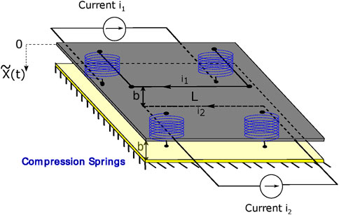
Figure 1. magMEMS with current-carrying filaments. The instantaneous distance between filaments is $b-\tilde{x}(t)$.

Note that the governing differential Equation 3 does not include a damping term as the air resistance is assumed to be negligible. This assumption is typically valid for sufficiently small MEMS devices, for example, Rhoads [33], Gorelick et al. [34], and references therein. However, in practical applications where damping effects cannot be neglected or to extend the model’s applicability, a damping term can be incorporated as discussed in Section 3.

Furthermore, it is a common practice to rescale the single-degree-of-freedom Equation 3 to facilitate interpretation. To this end, we introduce the following dimensionless distance and time variables

$x=\frac{\tilde{x}}{b}\text{and}t=\tilde{t}\sqrt{\frac{k_s}{m}},(4)$

respectively, in Equation 4. The transformation yields the following dimensionless form of the governing Equation 5:

$\ddot{x}+x-K\left[\frac{{\xi }^2\left(1-x\right)}{\sqrt{{\xi }^2{\left(1-x\right)}^2+1}}+\frac{1}{\left(1-x\right)\sqrt{{\xi }^2{\left(1-x\right)}^2+1}}-\xi \right]=0,(5)$

and the excitation parameter $K$ is defined in Equation 6:

$K=\frac{{\mu }_0{\mu }_r{i}_1{i}_{2}L}{2\pi k_s{b}^2},(6)$

and the dimensionless geometric parameter is given by

$\xi =\frac{b}{L}.$

Finally, we complement Equation 5 with zero initial conditions

$x\left(0\right)=\dot{x}\left(0\right)=0,$

and additionally, we assume that the currents in both wires are unidirectional, that is, $K\ge 0$.

It should be noted that Equation 5 reduces to

$\ddot{x}+x-\frac{K}{1-x}=0,(7)$

in the case where the filament’s motion is driven by the magnetic field of an infinite current-carrying conductor, that is, $\xi \to 0^{+}$. For $\xi =0$, the initial value problem described in Equation 7 under zero initial conditions exhibits periodic solutions when $K<K_0^{*}$; otherwise, it leads to pull-in behavior. Consequently, the dynamic pull-in threshold $K_0^{*}$ and the corresponding maximum deflection $A_0^{*}$ are given in He et al. [9] as Equation 8

$K_0^{*}=0.203632188\dots ,(8)$

and

$A_0^{*}=\frac{1+\sqrt{1-4K_0^{*}}}{2}=0.71533\dots ,$

respectively. In addition, the dynamic pull-in threshold $K_0^{*}$ and the maximum amplitude $A_0^{*}$ can also be calculated using the Lambert W function, as demonstrated in our previous work (Skrzypacz et al. [35]).

Next, multiplying both sides of Equation 5 by $\dot{x}$ and then integrating with respect to $t$ yields the conservation of the energy Equation 9:

$\begin{array}{cc}\hfill {\mathcal{E}}_{K,\xi }\left(t\right)& =\frac{1}{2}{\left(\dot{x}\left(t\right)\right)}^2+\frac{1}{2}{x}^2\left(t\right)\hfill \\ \hfill & -K\left[-\sqrt{{\xi }^2{\left(1-x\left(t\right)\right)}^2+1}+\mathrm{a}\mathrm{r}\mathrm{t}\mathrm{a}\mathrm{n}\mathrm{h}\left(\frac{1}{\sqrt{{\xi }^2{\left(1-x\left(t\right)\right)}^2+1}}\right)-\xi x\left(t\right)\right]\hfill \\ \hfill & -K\left[\sqrt{1+{\xi }^2}-\mathrm{a}\mathrm{r}\mathrm{t}\mathrm{a}\mathrm{n}\mathrm{h}\left(\frac{1}{\sqrt{1+{\xi }^2}}\right)\right],\hfill \end{array}(9)$

from which it follows Equation 10:

$\begin{array}{cc}\hfill {\left(\dot{x}\left(t\right)\right)}^2=& -x^2\left(t\right)\hfill \\ \hfill & +2K\left[-\sqrt{{\xi }^2{\left(1-x\left(t\right)\right)}^2+1}+\mathrm{a}\mathrm{r}\mathrm{t}\mathrm{a}\mathrm{n}\mathrm{h}\left(\frac{1}{\sqrt{{\xi }^2{\left(1-x\left(t\right)\right)}^2+1}}\right)-\xi x\left(t\right)\right]\hfill \\ \hfill & +2K\left[\sqrt{1+{\xi }^2}-\mathrm{a}\mathrm{r}\mathrm{t}\mathrm{a}\mathrm{n}\mathrm{h}\left(\frac{1}{\sqrt{1+{\xi }^2}}\right)\right].\hfill \end{array}(10)$

As noted previously by He et al. [9] and Skrzypacz et al. [10], the solution $x(t)$ is periodic if the phase portrait in the $(x,\dot{x})$ plane forms a closed curve, and the corresponding graph of the energy conservation equation, Equation 10, is also closed. This occurs when Equation 11

$\begin{array}{cc}\hfill f_{K,\xi }\left(s\right)& =-s^2+2K\left[-\sqrt{{\xi }^2{\left(1-s\right)}^2+1}+\mathrm{a}\mathrm{r}\mathrm{t}\mathrm{a}\mathrm{n}\mathrm{h}\left(\frac{1}{\sqrt{{\xi }^2{\left(1-s\right)}^2+1}}\right)-\xi s\right]\hfill \\ \hfill & +2K\left[\sqrt{1+{\xi }^2}-\mathrm{a}\mathrm{r}\mathrm{t}\mathrm{a}\mathrm{n}\mathrm{h}\left(\frac{1}{\sqrt{1+{\xi }^2}}\right)\right]\hfill \end{array}(11)$

has a root in the interval $(\mathrm{0,1})$. The operation of magnetic MEMS or magMEMS using filament wires of finite length can be described by Equation 5. For the case of $\xi =0$, the existence of periodic solutions is ensured if Equation 12

$f_{K,0}\left(s\right)=-s^2-2K\ln \left(1-s\right)(12)$

has a root in the interval $(\mathrm{0,1})$ (He et al. [9]). The first root corresponds to the maximum value of $x(t)$, that is, the maximum deflection of the oscillating component. Consequently, the solutions to the magMEMS model given by Equation 5 are periodic if $K<K_0^{*}$ and exhibit dynamic pull-in behavior if $K>K_0^{*}$, where it has been previously established that $K_0^{*}=0.203632188\dots$.

On the other hand, in the critical case $K=K_{\xi }^{*}$, the function $f_{K,\xi }(s)$ has a double root at $s=A_{\xi }^{*}$.

This condition is satisfied when

$f_{K_{\xi }^{*},\xi }\left(A_{\xi }^{*}\right)=0\text{and}\frac{\partial f_{K_{\xi }^{*},\xi }}{\partial s}\left(A_{\xi }^{*}\right)=0.$

which leads to the following transcendental Equation 13 for $A_{\xi }^{*}$:

$\begin{array}{cc}\hfill & \frac{A_{\xi }^{*}}{2}\left[\frac{{\xi }^2\left(1-A_{\xi }^{*}\right)}{\sqrt{{\xi }^2{\left(1-A_{\xi }^{*}\right)}^2+1}}+\frac{1}{\left(1-A_{\xi }^{*}\right)\sqrt{{\xi }^2{\left(1-A_{\xi }^{*}\right)}^2+1}}-\xi \right]\hfill \\ \hfill & =-\sqrt{{\xi }^2{\left(1-A_{\xi }^{*}\right)}^2+1}+\mathrm{a}\mathrm{r}\mathrm{t}\mathrm{a}\mathrm{n}\mathrm{h}\left(\frac{1}{\sqrt{{\xi }^2{\left(1-A_{\xi }^{*}\right)}^2+1}}\right)-\xi A_{\xi }^{*}\hfill \\ \hfill & +\sqrt{1+{\xi }^2}-\mathrm{a}\mathrm{r}\mathrm{t}\mathrm{a}\mathrm{n}\mathrm{h}\left(\frac{1}{\sqrt{1+{\xi }^2}}\right).\hfill \end{array}(13)$

The value of $A_{\xi }^{*}$, representing the maximum deflection, is obtained numerically for various values of the parameter $\xi$ by solving Equation 13. Once $A_{\xi }^{*}$ is known, the corresponding dynamic pull-in threshold $K_{\xi }^{*}$ can be calculated using Equation 14:

$K_{\xi }^{*}={\left[\frac{{\xi }^2\left(1-A_{\xi }^{*}\right)}{\sqrt{{\xi }^2{\left(1-A_{\xi }^{*}\right)}^2+1}}+\frac{1}{\left(1-A_{\xi }^{*}\right)\sqrt{{\xi }^2{\left(1-A_{\xi }^{*}\right)}^2+1}}-\xi \right]}^{-1}{A}_{\xi }^{*},(14)$

which follows from the condition $\frac{\partial f_{K_{\xi }^{*},\xi }}{\partial s}(A_{\xi }^{*})=0$. Figure 2 illustrates the effect of the geometry parameter $\xi$ on both the maximum deflection $A_{\xi }^{*}$ of the flexible part and the dynamic pull-in threshold $K_{\xi }^{*}$. As $\xi$ increases, the maximum deflection $A_{\xi }^{*}$ decreases due to a weakening Lorentz force. Conversely, the dynamic pull-in threshold $K_{\xi }^{*}$ increases with increasing $\xi$ for the same reason.

Figure 2

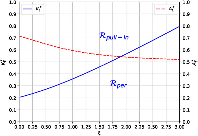
Figure 2. Dynamic pull-in threshold $K_{\xi }^{*}$ and maximum deflection $A_{\xi }^{*}$ of the flexible part. Pairs $(\xi ,K)$ below the separatrix $K^{*}=K_{\xi }^{*}$ (region ${\mathcal{R}}_{\mathit{per}}$) lead to periodic solutions.

In the regime of small values of the geometric parameter $\xi$, an asymptotic expansion yields the following approximation for the function $f_{K,\xi }^{\prime }(s)$ developed by Skrzypacz et al. [10]:

$f_{K,\xi }\left(s\right)=-s^2-2K\log |1-x|-2Ks\xi -\frac{1}{2}Ks\left(s-2\right){\xi }^2+\mathcal{O}\left({\xi }^4\right)$

with its derivative given by

$f_{K,\xi }^{\prime }\left(s\right)=-2s+\frac{2K}{1-x}-2K\xi -\frac{1}{2}K\left(2s-2\right){\xi }^2+\mathcal{O}\left({\xi }^4\right).$

To facilitate further analysis, we introduce the simplified function in Equation 15:

${\tilde{f}}_{K,\xi }\left(s\right)=-s^2-2K\log |1-s|-2K\xi s-\frac{1}{2}K\xi s{\left(s-2\right)}^2,(15)$

which captures the leading-order behavior of $f_{K,\xi }^{\prime }(s)$ for small $\xi$. Under this approximation, the motion of the platform is governed by the second-order nonlinear differential equation:

$\ddot{y}=\frac{1}{2}{\tilde{f}}_{K,\xi }^{\prime }\left(y\right).$

This leads to approximate model Equation 16 for the magnetic MEMS:

$\ddot{y}+\left(1+\frac{K{\xi }^2}{2}\right)y=\frac{K}{1-y}-K\xi +\frac{K{\xi }^2}{2},(16)$

subject to the initial conditions Equation 17:

$y\left(0\right)=0,\dot{y}\left(0\right)=0.(17)$

In the presence of damping effects, this equation can be generalized to Equation 18:

$\ddot{y}+\gamma \dot{y}+\left(1+\frac{K{\xi }^2}{2}\right)y=\frac{K}{1-y}-K\xi +\frac{K{\xi }^2}{2},(18)$

where $\gamma \ge 0$ is the dimensionless damping coefficient. In what follows, we apply the Galerkin method to compute periodic solutions of the magMEMS model described in Equations 16, 17 and subsequently extend the analysis to include damping effects.

3 Dynamical model analysis via the Galerkin approach

In this section, we apply the Galerkin approach to approximate periodic solutions of the magMEMS model, first in the undamped case and subsequently in the presence of damping.

3.1 Undamped case $(\gamma =0)$

Let us rewrite Equation 16 as follows:

$\left(1-y\right)\ddot{y}-\left(1+\frac{K{\xi }^2}{2}\right)y^2+\left(1-K\xi +K{\xi }^2\right)y-K+K\xi -\frac{K{\xi }^2}{2}=0.$

To obtain the weak formulation, we need to find periodic $y$ satisfying the initial conditions by Equation 17 such that

$\underset{0}{\overset{T}{\int }}\left[\left(1-y\right)\ddot{y}-\left(1+\frac{K{\xi }^2}{2}\right)y^2+\left(1-K\xi +K{\xi }^2\right)y-K+K\xi -\frac{K{\xi }^2}{2}\right]v\mathrm{d}t=0(19)$

holds for all $v\in L^2(0,T)$. We seek a Galerkin approximation in the form

$\tilde{y}\left(t\right)=a\left(1-\cos \left(\omega t\right)\right).(20)$

Note that the periodic Galerkin ansatz by Equation 20 satisfies the initial conditions

$\tilde{y}\left(0\right)=0,\dot{\stackrel{̃}{y}}\left(t\right)=a\omega \sin \left(\omega t\right)\Rightarrow \dot{\stackrel{̃}{y}}\left(0\right)=0.$

Substituting the corresponding Galerkin ansatz into the weak formulation in Equation 19 and testing over one period $T=2\pi /\omega$ with test functions $v\in span\{1,\cos (\omega t)\}$ yields the following algebraic system:

$\begin{array}{cc}\hfill \left(-2{\omega }^2+3K{\xi }^2+6\right)a^2+\left(-4-4K{\xi }^2+4K\xi \right)a+2K{\xi }^2-4K\xi +4K& =0,\hfill \\ \hfill Ka{\xi }^2-K{\xi }^2-a{\omega }^2+K\xi +{\omega }^2+2a-1& =0.\hfill \end{array}(21)$

From the second equation in Equation 21, we obtain Equation 22:

${\omega }^2={\omega }_{K,\xi }^2=\frac{1-2a-Ka{\xi }^2+K{\xi }^2-K\xi }{1-a}.(22)$

As

$\tilde{y}\left(t\right)=a\left(1-\cos \left(\omega t\right)\right)=2a{\sin }^2\left(\frac{\omega t}{2}\right),$

the maximal deflection is $2a$, and the requirement $x\le 1$ imposes $a\le \frac{1}{2}$. Substituting ${\omega }^2$ by Equation 22 into the first equation of Equation 21 yields Equation 23:

$a^3+\frac{-5K{\xi }^2+2K\xi -8}{K{\xi }^2+2}{a}^2+\frac{6K{\xi }^2-8K\xi +4K+4}{K{\xi }^2+2}a+\frac{-2K{\xi }^2+4K\xi -4K}{K{\xi }^2+2}=0.(23)$

Here, $K>0$, $\xi \ge 0$, and $0<a\le \frac{1}{2}$ result from the Galerkin ansatz. The roots of the cubic Equation 23 can be expressed in the following trigonometric form as presented in Equation 24 [36]:

$\begin{array}{ll}\hfill a_{\ell }& =2\sqrt{-\frac{q-\frac{p^2}{3}}{3}}\cos \left(\frac{1}{3}\arccos \left(\frac{3\left(r-\frac{pq}{3}+\frac{2p^3}{27}\right)}{2\left(q-\frac{p^2}{3}\right)}\sqrt{-\frac{3}{q-\frac{p^2}{3}}}\right)+\frac{2\pi \ell }{3}\right)\hfill \\ \hfill & -\frac{p}{3},\ell =\mathrm{0,1,2},\hfill \end{array}(24)$

where Equation 25

$p=\frac{-5K{\xi }^2+2K\xi -8}{K{\xi }^2+2},q=\frac{6K{\xi }^2-8K\xi +4K+4}{K{\xi }^2+2},r=\frac{-2K{\xi }^2+4K\xi -4K}{K{\xi }^2+2},(25)$

and Equation 26

${\mathrm{\Delta }}_{K,\xi }=-4{\left(q-\frac{p^2}{3}\right)}^3-27{\left(r-\frac{pq}{3}+\frac{2p^3}{27}\right)}^2\ge 0.(26)$

In our case, we obtain Equation 27:

$\begin{array}{cc}\hfill a_{K,\xi }=a_1& =\frac{2\sqrt{\left(7{\xi }^4+4{\xi }^3-8{\xi }^2\right)K^2+\left(32{\xi }^2+16\xi -24\right)K+40}}{3\left(K{\xi }^2+2\right)}\hfill \\ \hfill & \cos \left(\frac{1}{3}\arccos \left({\beta }_{K,\xi }\right)+\frac{2\pi }{3}\right)-\frac{-5K{\xi }^2+2K\xi -8}{3\left(K{\xi }^2+2\right)},\hfill \end{array}(27)$

where (Equation 28)

$\begin{array}{cc}\hfill {\beta }_{K,\xi }& =\frac{\left(17{\xi }^3+30{\xi }^2-48\xi +28\right)K^3{\xi }^3+\left(132{\xi }^3+96{\xi }^2-156\xi +72\right)K^2\xi }{{\left(7K^2{\xi }^4+4K^2{\xi }^3-8K^2{\xi }^2+32K{\xi }^2+16K\xi -24K+40\right)}^{3/2}}\hfill \\ \hfill & +\frac{\left(312{\xi }^2+48\xi -72\right)K+224}{{\left(7K^2{\xi }^4+4K^2{\xi }^3-8K^2{\xi }^2+32K{\xi }^2+16K\xi -24K+40\right)}^{3/2}}.\hfill \end{array}(28)$

The condition ${\mathrm{\Delta }}_{K,\xi }=0$, that is, Equation 29

$\begin{array}{cc}\hfill 0& =\left({\xi }^8-8{\xi }^7-2{\xi }^6+12{\xi }^5-56{\xi }^4+64{\xi }^3-24{\xi }^2\right)K^4\hfill \\ \hfill & +\left(-32{\xi }^5+48{\xi }^4-160{\xi }^3-48{\xi }^2+176\xi -64\right)K^3\hfill \\ \hfill & +\left(-16{\xi }^4+64{\xi }^3+16{\xi }^2-544\xi +296\right)K^2+\left(256\xi -384\right)K+64\hfill \end{array}(29)$

constitutes the approximate separatrix.

If $\xi =0$, that is, the wire is infinite, we obtain Equation 30:

$a=a_{K,0}=\frac{2\sqrt{10-6K}}{3}\cos \left(\frac{1}{3}\arccos \left(\frac{28-9K}{{\left(10-6K\right)}^{3/2}}\right)+\frac{2\pi }{3}\right)+\frac{4}{3}.(30)$

Note that the discriminant condition ${\mathrm{\Delta }}_{K,0}=32\left(K^3-\frac{37}{8}{K}^2+6K-1\right)=0$ for cubic Equation 23 ensures that its two roots coincide for $\xi =0$. This corresponds to the approximate pull-in case, where the approximate pull-in threshold is ${\tilde{K}}_0^{*}=0.19464$. This critical value is very close to the exact dynamic pull-in threshold $K_0^{*}$ given by Equation 8. The approximate periodic solutions are given for $0<K<{\tilde{K}}_0^{*}$ as shown in Equation 31:

$\tilde{y}\left(t\right)=2a_{K,0}{\sin }^2\left(\frac{t}{2}\sqrt{\frac{1-2a_{K,0}}{1-a_{K,0}}}\right),(31)$

where the $K$-dependent coefficient $a_{K,0}$ is defined by Equation 30.

Note that the ansatz in Equation 20 can be systematically extended by incorporating additional terms from the Fourier expansion. For instance, a single-term ansatz with adaptive coefficients may reduce computational effort without compromising accuracy, which is consistent with minimalist modeling principles in MEMS analysis. However, increasing the number of trigonometric terms in the ansatz inevitably results in higher-order nonlinear algebraic systems, which must be solved using numerical methods. Accurate models are essential for capturing the nonlinear dynamics of oscillators. Among the notable analytical–semi-analytical techniques are the VIM [37] and the HPM [38, 39]. VIM is particularly effective in treating strongly nonlinear systems and has been successfully used to predict pull-in conditions in electrostatic MEMS. HPM, a semi-analytical method that combines homotopy theory with perturbation techniques, offers robust solutions to problems with not well-defined initial guesses. It is especially suitable for complex nonlinear scenarios as it can transform intricate governing equations into tractable forms more efficiently than many traditional approaches [37–39]. Recently, He’s frequency formula and Ma’s modification have been applied to the analysis of fractal vibration systems [40]. Both VIM and HPM demonstrated the capability to yield approximate pull-in thresholds with relatively high accuracy [18, 41]. For example, J.-H. He, in [18], used VIM to determine the approximate pull-in threshold for the magMEMS oscillator in the case of an infinitely long wire $(\xi =0)$, obtaining the value $K^{*}=0.20498$ for $K_0^{*}$, corresponding to a relative error of less than $1\%$.

3.2 Damped case $(\gamma >0)$

Let us rewrite Equation 18 as follows:

$\left(1-y\right)\ddot{y}+\gamma \left(1-y\right)\dot{y}-\left(1+\frac{K{\xi }^2}{2}\right)y^2+\left(1-K\xi +K{\xi }^2\right)y-K+K\xi -\frac{K{\xi }^2}{2}=0.$

To obtain the weak formulation for the damped case, we need to find a periodic $y$ satisfying the initial conditions by Equation 17 such that Equation 32

$\begin{array}{ll}\hfill & \underset{0}{\overset{T}{\int }}\left[\left(1-y\right)\ddot{y}+\gamma \left(1-y\right)\dot{y}-\left(1+\frac{K{\xi }^2}{2}\right)y^2+\left(1-K\xi +K{\xi }^2\right)y-K+K\xi -\frac{K{\xi }^2}{2}\right]\hfill \\ \hfill & v\mathrm{d}t=0\hfill \end{array}(32)$

holds for all $v\in L^2(0,T)$.

We seek a Galerkin approximation that includes both transient damping effects and the correct steady-state behavior. Let $y_{ss}$ denote the steady-state solution satisfying the equilibrium Equation 33:

$\left(1+\frac{K{\xi }^2}{2}\right)y_{ss}=\frac{K}{1-y_{ss}}-K\xi +\frac{K{\xi }^2}{2},(33)$

which follows from Equation 18 assuming $\ddot{y}=\dot{y}=0$.

The Galerkin ansatz takes the form, as shown in Equation 34:

$\tilde{y}\left(t\right)=y_{ss}\left(1-e^{-\alpha t}\right)+a{e}^{-\alpha t}\left(1-\cos \left({\omega }_{d}t\right)\right),(34)$

where $\alpha$ is the decay rate, ${\omega }_d$ is the damped frequency, and $a$ is the Galerkin coefficient from the undamped analysis. This formulation ensures that $\tilde{y}(0)=0$ and ${\lim }_{t\to \infty }\tilde{y}(t)=y_{ss}$.

For the damped case, we use ${\omega }_d={\omega }_0$ and $\alpha =\gamma /2$, with $y_{ss}$ found numerically from Equation 33. The formulation captures both transient and steady-state behaviors, converging to the equilibrium position $y_{ss}$. For the pull-in threshold, we approximate Equation 35:

${\mathrm{\Delta }}_{K,\xi ,\gamma }\approx {\mathrm{\Delta }}_{K,\xi ,0}-\mathcal{O}\left({\gamma }^2\right)\ge 0.(35)$

This leads to the damped pull-in threshold, as shown in Equation 36:

${\tilde{K}}_{\xi ,\gamma }^{*}={\tilde{K}}_{\xi ,0}^{*}+\mathcal{O}\left({\gamma }^2\right).(36)$

This formulation recovers the undamped solution as $\gamma \to 0$ and provides accurate predictions for practical magMEMS applications, where $\gamma \ll 1$.

Figure 3 shows a comparison between undamped and damped solutions. The plots demonstrate how damping affects transient behavior while maintaining correct steady-state convergence. Galerkin approximations (solid lines) match numerical ODE solutions (dashed lines).

Figure 3

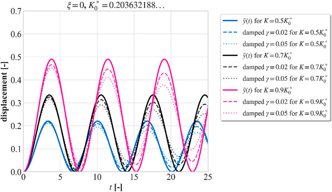
Figure 3. Comparison between undamped and damped magMEMS solutions for different excitation parameters. It shows how damping affects transient behavior while maintaining correct steady-state convergence. Galerkin approximations (solid lines) match numerical ODE solutions (dashed lines).

The accuracy of the Galerkin formulation is demonstrated in Figure 4, which compares numerical ODE solutions with analytical Galerkin approximations. The upper subplot shows the time evolution of both solutions, whereas the lower subplot displays the absolute error between them.

Figure 4

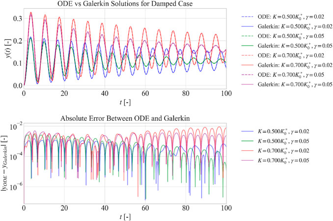
Figure 4. Comparison between numerical ODE solutions and analytical Galerkin approximations. The upper subplot shows the time evolution of both solutions. The lower subplot displays the absolute error, demonstrating the accuracy of analytical approximation.

Figure 5 shows the effect of damping on the maximum amplitude as a function of excitation parameter $K$. Damped solutions show reduced amplitudes compared to the undamped case, particularly as $K$ approaches the pull-in threshold, demonstrating the stabilizing effect of damping.

Figure 5

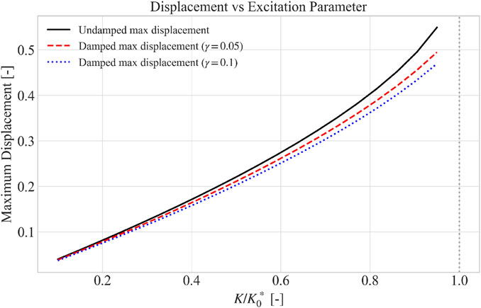
Figure 5. Effect of damping on maximum displacement as a function of the excitation parameter $K$. Damped solutions show reduced amplitudes compared to undamped cases, particularly near pull-in threshold, demonstrating the stabilizing effect of damping.

4 Discussion and simulation results

In this section, we present numerical simulations of the normalized deflection of the platform, $y(t)$, as a function of nondimensional time $t$. We analyze the behavior of the periodic solution $y(t)$ under different sets of parameters $K>0$ and $\xi \ge 0$. The simulations were performed using Maple™ software [42], and the resulting deflection profiles are illustrated in Figures 6–8. The observed trends clearly reveal the dependency of the deflection amplitude, frequency, and pull-in time on the excitation parameter $K$ while keeping the geometric parameter $\xi$ fixed. In particular, an increase in the value of $K$ leads to a larger amplitude and a longer period of deflection. In particular, for the given value of the geometric parameter $\xi \ge 0$, the maximum deflection is attained when $K$ approaches the threshold value $K_{\xi }^{*}$. In Figures 6–8, the periodic solutions with the highest deflection correspond to the excitation value $K=0.9K_{\xi }^{*}$.

Figure 6

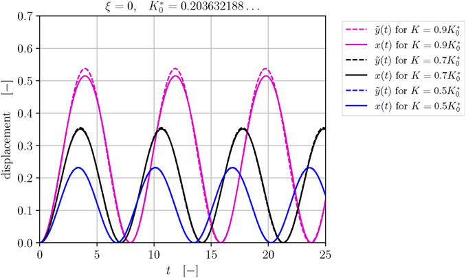
Figure 6. Profiles of Galerkin solutions $\tilde{y}(t)$ (dashed lines) for $\xi =0$ and $K=0.9K_0^{*};0.7K_0^{*};0.5K_0^{*}$. Solid lines corresponds to numerical reference solutions $x(t)$ of Equation 5, which for $\xi =0$ coincides with the approximate model given by Equation 16.

Figure 7

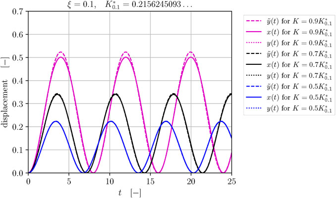
Figure 7. Profiles of Galerkin solutions $\tilde{y}(t)$ (dashed lines) for $\xi =0.1$ and $K=0.9K_{0.1}^{*};0.7K_{0.1}^{*};0.5K_{0.1}^{*}$. Solid lines correspond to numerical reference solutions $x(t)$ of Equation 5, whereas dot lines correspond to numerical solution $y(t)$ of the approximate model given in Equation 16.

Figure 8

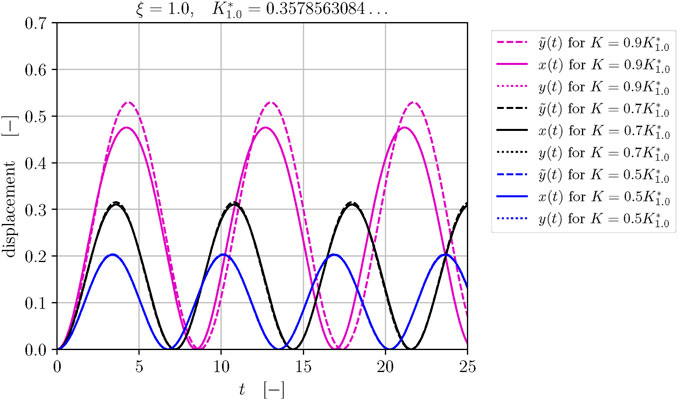
Figure 8. Profiles of Galerkin solutions $\tilde{y}(t)$ (dashed lines) for $\xi =1.0$ and $K=0.9K_{1.0}^{*};0.7K_{1.0}^{*};0.5K_{1.0}^{*}$. Solid lines correspond to the numerical reference solutions $x(t)$ of Equation 5, whereas dot lines correspond to the numerical solution $y(t)$ of the approximate model given by Equation 16.

Note that the range of dimensionless parameters $K$ and $\xi$ is already broad enough in this study for practical applications. In the case of arbitrary $K>0$ and $\xi \ge 0$, the trajectories and their approximations can be studied using the Maple™ and Python scripts available at https://github.com/armanbolatov/magmems_damping.

Furthermore, as the value of $\xi$ increases, the maximum deflection diminishes due to the weakened Lorentz force. In Figure 9, the approximate separatrix ${\tilde{K}}_{\xi }^{*}$, defined by Equation 29, is compared with the exact separatrix $K_{\xi }^{*}$ as functions of the geometric parameter $\xi$. The approximate separatrix slightly underestimates the dynamic pull-in threshold in the $\xi$-parameter range [0,1.2]. The study clearly demonstrates that the pull-in threshold, $K_{\xi }^{*}$, depends sensitively on the geometric parameter $\xi$. As $\xi$ increases, corresponding to shorter filament lengths, the pull-in threshold $K_{\xi }^{*}$ increases, whereas the maximum deflection amplitude $A_{\xi }^{*}$ decreases. Numerical simulations confirm this inverse relationship between $K_{\xi }^{*}$ and $A_{\xi }^{*}$. For the case of infinite filaments $(\xi =0)$, the threshold is approximately $K_0^{*}\approx 0.2036$, providing a quantitative reference for designers to mitigate pull-in instability.

Figure 9

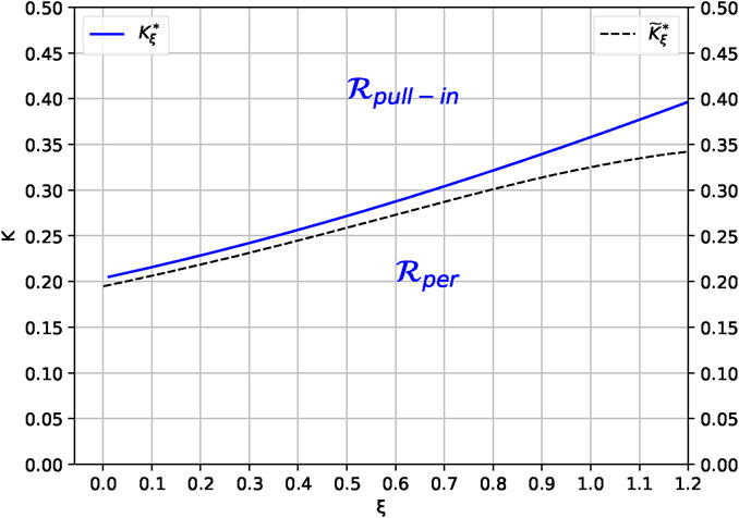
Figure 9. Exact and approximate separatrix. Pairs $(\xi ,K)$ below exact separatrix $K_{\xi }^{*}$ (region ${\mathcal{R}}_{\mathit{per}}$) lead to periodic solutions.

The exact (harmonic) frequency of oscillations is defined as shown in Equation 37:

${\omega }_{K,\xi }^{ex}=\frac{2\pi }{T_{K,\xi }},(37)$

where $T_{K,\xi }$ denotes the exact period of oscillations. Integrating Equation 10 yields Equation 38:

$\frac{T_{K,\xi }}{2}=\underset{0}{\overset{A_{K,\xi }}{\int }}\frac{ds}{\sqrt{f_{K,\xi }\left(s\right)}},(38)$

where $A_{K,\xi }$ is the maximum displacement for the given parameter pair $K>0$ and $\xi \ge 0$ such that $K<K_{\xi }^{*}$. The value $A_{K,\xi }$ is the first positive root of $f_{K,\xi }(s)$, defined in Equation 11 for $\xi >0$ and in Equation 12 for $\xi =0$. The integrals in Equation 38 are computed numerically. In Table 1, the high-precision values of frequencies computed using Equation 37 are compared with their Galerkin approximations given by Equation 22. We observe that for the geometric parameter $\xi =0.1$, the Galerkin approximation results in an absolute error in frequencies of order $10^{-3}$, even for the value of excitation parameter $K$, close to the pull-in threshold. The accuracy improves for the smaller values of $K$ and $\xi$. The decrease in the period approximation accuracy for larger values of the geometric parameter $\xi$ and values of excitation parameter $K$ close to the pull-in threshold can be well observed in Figure 8.

Table 1

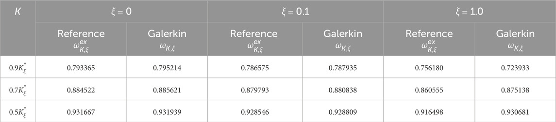
Table 1. High-precision frequencies ${\omega }_{K,\xi }^{ex}$ and their Galerkin approximations ${\omega }_{K,\xi }$ for $K=0.9K_{\xi }^{*};0.7K_{\xi }^{*};0.5K_{\xi }^{*}$ and $\xi =0;0.1;1.0$.

In Figure 10, the maximal displacement and its Galerkin approximation is presented versus varying excitation parameter K for ξ = 0; 0.1; 1.0. The Galerkin approximation of the maximum displacement is close to its exact value for small values of the geometric parameter ξ.

Figure 10

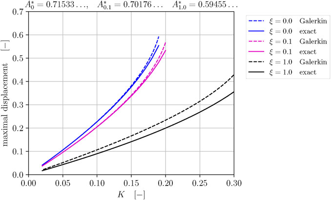
Figure 10. Exact and Galerkin approximations of maximum displacements for $\xi =0;0.1;1.0$and varying $K$.

5 Conclusions and outlooks

In this paper, the Galerkin approach is used to derive approximate expressions for the pull-in threshold, oscillation frequency, and periodic solutions of the magMEMS. It has been demonstrated that these approximations maintain a high degree of accuracy for excitation parameters below the critical pull-in value, denoted by $K_{\xi }^{*}$.

Furthermore, we have extended the analysis to include damping effects for the small damping coefficient $\gamma \ll 1$ through an improved Galerkin formulation that incorporates both transient decay and correct steady-state behavior. The enhanced ansatz ensures convergence to the physically appropriate equilibrium position while maintaining the zero initial condition for displacement and recovers the undamped solution in the limit as the damping coefficient tends to zero. The method has proven to be of particular value in the domains of MEMS design and performance estimation, offering a combination of analytical depth and practical implementability. By formulating the nonlinear governing equation in its weak form and using a periodic cosine ansatz, closed-form approximations for the dynamic pull-in threshold, oscillation frequency, and periodic solutions have been obtained. This approach represents a significant advancement as it mitigates the computational demands associated with conventional numerical techniques (e.g., shooting or continuation methods) while preserving high accuracy suitable for engineering applications. The Galerkin-based solutions effectively capture the influence of the excitation parameter on the system’s dynamic response. Moreover, unlike purely numerical ODE solutions, they provide deeper insights into the interplay between excitation and geometric parameters governing oscillator dynamics. Increasing the excitation parameter leads to larger maximal deflections and a concomitant elongation of the oscillation period. Conversely, increasing the geometric parameter diminishes deflections by attenuating the Lorentz forces. In particular, for the geometric parameter $\xi =0.1$, frequency approximations exhibit errors as low as $10^{-3}$, thereby validating the robustness and precision of the method. The analysis also reveals effective strategies for controlling the system’s dynamic behavior, enabling the avoidance of pull-in instability. This comprehensive analysis contributes to a more profound understanding of the system and may serve as a catalyst for further research endeavors concerning related phenomena. The findings of the present study provide critical design guidelines to optimize magMEMS performance for wearable sensor applications. By adjusting geometric parameters and excitation currents based on the derived pull-in thresholds, engineers can ensure the reliable operation of magnetically actuated wearable devices, including biomedical sensors and motion-tracking modules. This approach allows for the preservation of high sensitivity to external stimuli while maintaining robust functionality. The low-complexity nature of the Galerkin model further facilitates its integration into real-time control algorithms for wearable systems, addressing the power and computational constraints inherent in portable electronics. This work paves the way for the development of next-generation, reliable magMEMS-based wearable technologies that demand precise dynamic response and miniaturization.

Data availability statement

The source code and supplementary materials for this research are available at https://github.com/armanbolatov/magmems_damping.

Author contributions

LZ: Methodology, Investigation, Funding acquisition, Writing – review and editing. J-HH: Methodology, Writing – review and editing, Writing – original draft, Conceptualization, Funding acquisition, Validation. PS: Visualization, Formal Analysis, Project administration, Resources, Validation, Data curation, Methodology, Software, Supervision, Investigation, Conceptualization, Writing – review and editing, Writing – original draft, Funding acquisition. AB: Methodology, Investigation, Validation, Data curation, Software, Writing – original draft. DK: Writing – review and editing, Investigation, Methodology, Validation. GE: Methodology, Validation, Investigation, Writing – review and editing. BP: Validation, Methodology, Investigation, Writing – original draft, Writing – review and editing. PP: Writing – review and editing, Methodology, Formal Analysis, Writing – original draft, Investigation, Validation, Conceptualization.

Funding

The author(s) declare that financial support was received for the research and/or publication of this article. PS, AB, DK, and GE were supported by the Ministry of Education and Science of the Republic of Kazakhstan within the framework of Project AP19676969. The work is funded by the National Foreign Experts Program of the Ministry of Education (G2023014001L), the Technology Innovation Team of Yancheng Polytechnic College (YGKJ202502), and the doctoral research initiation fund project of Yancheng Polytechnic College (2023). The key technology innovation platform for flame retardant fiber and functional textiles in Jiangsu Province (2022JMRH-003) also supports this research. PS and GE have been supported by the Ministry of Education and Science of the Republic of Kazakhstan within the framework of Project AP19676969 Modeling, Analysis, and Optimization of MEMS and magMEMS. PPu and BP have received funding from a project co-financed by the Polish Ministry of Science and Higher Education under the European Union’s Horizon Europe programme under Marie Skłodowska-Curie Actions–Staff Exchanges (SE) grant agreement No. 101086226-ENSIGN.

Conflict of interest

The authors declare that the research was conducted in the absence of any commercial or financial relationships that could be construed as a potential conflict of interest.

Generative AI statement

The author(s) declare that no Generative AI was used in the creation of this manuscript.

Any alternative text (alt text) provided alongside figures in this article has been generated by Frontiers with the support of artificial intelligence and reasonable efforts have been made to ensure accuracy, including review by the authors wherever possible. If you identify any issues, please contact us.

Publisher’s note

All claims expressed in this article are solely those of the authors and do not necessarily represent those of their affiliated organizations, or those of the publisher, the editors and the reviewers. Any product that may be evaluated in this article, or claim that may be made by its manufacturer, is not guaranteed or endorsed by the publisher.

Footnotes

¹This quantity is also called the co-energy of the magnetic field.

References

1. Younis MI MEMS linear and nonlinear statics and dynamics, 20. Springer Science & Business Media (2011).

Google Scholar

2. Li W, Zhao X, Cai B, Zhou G, Zhang M. Magnetically actuated mems variable optical attenuator. Micromachining Microfabrication Process Technology Devices (SPIE) (2001) 4601:89–96. doi:10.1117/12.444689

CrossRef Full Text | Google Scholar

3. Gao W, Emaminejad S, Nyein HYY, Challa S, Chen K, Peck A, et al. Fully integrated wearable sensor arrays for multiplexed in situ perspiration analysis. Nature (2016) 529:509–14. doi:10.1038/nature16521

PubMed Abstract | CrossRef Full Text | Google Scholar

4. Amjadi M, Kyung K-U, Park I, Sitti M. Stretchable, skin-mountable, and wearable strain sensors and their potential applications: a review. Adv Funct Mater (2016) 26:1678–98. doi:10.1002/adfm.201504755

CrossRef Full Text | Google Scholar

5. Masoud M, Jaradat Y, Manasrah A, Jannoud I. Sensors of smart devices in the internet of everything (ioe) era: big opportunities and massive doubts. J Sensors (2019) 2019:1–26. doi:10.1155/2019/6514520

CrossRef Full Text | Google Scholar

6. Iannacci J. Microsystem based energy harvesting (eh-mems): powering pervasivity of the internet of things (iot)–a review with focus on mechanical vibrations. J King Saud University-Science (2019) 31:66–74. doi:10.1016/j.jksus.2017.05.019

CrossRef Full Text | Google Scholar

7. Babij M, Majstrzyk W, Sierakowski A, Janus P, Grabiec P, Ramotowski Z, et al. Mems displacement generator for atomic force microscopy metrology. Meas Sci Technology (2021) 32:065903. doi:10.1088/1361-6501/abc28a

CrossRef Full Text | Google Scholar

8. Pruchnik B, Orłowska K, Świadkowski B, Gacka E, Sierakowski A, Janus P, et al. Microcantilever-based current balance for precise measurement of the photon force. Scientific Rep 2023 (2023) 13(13):466–9. doi:10.1038/s41598-022-27369-3

PubMed Abstract | CrossRef Full Text | Google Scholar

9. He J-H, Nurakhmetov D, Skrzypacz P, Wei D. Dynamic pull-in for micro–electromechanical device with a current-carrying conductor. J Low Frequency Noise, Vibration Active Control (2021) 40:1059–66. doi:10.1177/1461348419847298

CrossRef Full Text | Google Scholar

10. Skrzypacz P, Ellis G, He J-H, He C-H. Dynamic pull-in and oscillations of current-carrying filaments in magnetic micro-electro-mechanical system. Commun Nonlinear Sci Numer Simulation (2022) 109:106350. doi:10.1016/j.cnsns.2022.106350

CrossRef Full Text | Google Scholar

11. Yang Q. A mathematical control for the pseudo-pull-in stability arising in a micro-electromechanical system. J Low Frequency Noise, Vibration Active Control (2023) 42:927–34. doi:10.1177/14613484221133603

CrossRef Full Text | Google Scholar

12. He J-H, Yang Q, He C-H, Alsolami AA. Pull-down instability of the quadratic nonlinear oscillators. Facta Universitatis, Ser Mech Eng (2023) 21:191–200. doi:10.22190/fume230114007h

CrossRef Full Text | Google Scholar

13. He J-H, Bai Q, Luo Y-C, Kuangaliyeva D, Ellis G, Yessetov Y, et al. Modeling and numerical analysis for mems graphene resonator. Front Phys (2025) 13:1551969. doi:10.3389/fphy.2025.1551969

CrossRef Full Text | Google Scholar

14. Di Barba P, Wiak S. MEMS: field models and optimal design. Springer (2020).

Google Scholar

15. Ghourichaei M, Kerimzade U, Demirkazik L, Pruchnik B, Kwoka K, Badura D, et al. Multiscale fabrication and characterization of a nems force sensor. Adv Mater Tech (2024) 10:2400022. doi:10.1002/admt.202400022

CrossRef Full Text | Google Scholar

16. Yeatman E. Design and performance analysis of thermally actuated mems circuit breakers. J Micromechanics Microengineering (2005) 15:S109–15. doi:10.1088/0960-1317/15/7/016

CrossRef Full Text | Google Scholar

17. Rezazadeh G, Madinei H, Shabani R. Study of parametric oscillation of an electrostatically actuated microbeam using variational iteration method. Appl Math Model (2012) 36:430–43. doi:10.1016/j.apm.2011.07.026

CrossRef Full Text | Google Scholar

18. Anjum N, He J-H, He C-H, Gepreel KA. Variational iteration method for prediction of the pull-in instability condition of micro/nanoelectromechanical systems. Phys Mesomechanics (2023) 26:241–50. doi:10.1134/s1029959923030013

CrossRef Full Text | Google Scholar

19. Skrzypacz P, Ellis G, Pruchnik B, Putek P. Generalized analysis of dynamic pull-in for singular magmems and mems oscillators. Scientific Rep (2025) 15:23691. doi:10.1038/s41598-025-09515-9

PubMed Abstract | CrossRef Full Text | Google Scholar

20. Skrzypacz PS, Putek PA, Pruchnik BC, Turganov A, Ellis GA, Gotszalk TP. Analysis of dynamic pull-in for lumped mems model of atomic force microscope with constant magnetic excitation. J Sound Vibration (2025) 617:119215. doi:10.1016/j.jsv.2025.119215

CrossRef Full Text | Google Scholar

21. He J-H. Periodic solution of a micro-electromechanical system. Facta Universitatis, Ser Mech Eng (2024) 187–98. doi:10.22190/fume240603034h

CrossRef Full Text | Google Scholar

22. Nadeem M, Ain Q-T, Almakayeel N, Shao Y, Wang S, Shutaywi M. Analysis of nanobeam-based microstructure in n/mems system using van der waals forces. Facta Universitatis, Ser Mech Eng (2024) 673–88. doi:10.22190/fume240904048n

CrossRef Full Text | Google Scholar

23. Di Barba P, Fattorusso L, Versaci M Electrostatic field in terms of geometric curvature in membrane mems devices. Commun Appl Ind Math (2017) 8:165–84. doi:10.1515/caim-2017-0009

CrossRef Full Text | Google Scholar

24. Skrzypacz P, He J-H, Ellis G, Kuanyshbay M. A simple approximation of periodic solutions to microelectromechanical system model of oscillating parallel plate capacitor. Math Methods Appl Sci (2020) mma.6898–8. doi:10.1002/mma.6898

CrossRef Full Text | Google Scholar

25. He J-H, Skrzypacz PS, Zhang Y, Pang J. Approximate periodic solutions to microelectromechanical system oscillator subject to magnetostatic excitation. Math Methods Appl Sci (2020):mma.7018. doi:10.1002/mma.7018

CrossRef Full Text | Google Scholar

26. He C-H, He J-H, Ma J, Alsolami AA, Yang X-J. A modified frequency formulation for nonlinear mechanical vibrations. Facta Universitatis, Ser Mech Eng (2025) 23:197. doi:10.22190/fume250526022h

CrossRef Full Text | Google Scholar

27. Liu Y-P, He J-H. A fast and accurate estimation of amperometric current response in reaction kinetics. J Electroanalytical Chem (2025) 978:118884. doi:10.1016/j.jelechem.2024.118884

CrossRef Full Text | Google Scholar

28. He J-H, Ma J, Alsolami AA, He C-H, Yang XJ. Variational approach to micro-electro-mechanical systems. Facta Universitatis, Ser Mech Eng (2025) 23:197.

Google Scholar

29. Mohammadian M. Application of he’s new frequency-amplitude formulation for the nonlinear oscillators by introducing a new trend for determining the location points. Chin J Phys (2024) 89:1024–40. doi:10.1016/j.cjph.2024.03.047

CrossRef Full Text | Google Scholar

30. Omarov D, Nurakhmetov D, Wei D, Skrzypacz P. On the application of sturm’s theorem to analysis of dynamic pull-in for a graphene-based mems model. Appl Comput Mech (2018) 12. doi:10.24132/acm.2018.413

CrossRef Full Text | Google Scholar

31. Anjum N, He J-H. Geometric potential in nano/microelectromechanical systems: Part i mathematical model. Int J Geometric Methods Mod Phys (2024):2440027. doi:10.1142/s0219887824400279

CrossRef Full Text | Google Scholar

32. Griffiths DJ. Introduction to electrodynamics. Cambridge University Press (2023).

Google Scholar

33. Rhoads JF. Me 597: mechanics of mems and nems (2013). Available online at: https://engineering.purdue.edu/jfrhoads/ME597/Mechanics%20of%20MEMS%20and%20NEMS.pdf (Accessed May 26, 2025).

Google Scholar

34. Gorelick S, Dekker JR, Leivo M, Kantojärvi U. Air damping of oscillating mems structures: modeling and comparison with experiment. In: Proc. Comsol Conf. 1–5 (2013).

Google Scholar

35. Boyd JP. Solving transcendental equations: the Chebyshev polynomial proxy and other numerical rootfinders, perturbation series, and oracles. Society for Industrial and Applied Mathematics. (2014).

CrossRef Full Text | Google Scholar

36. Zucker IJ. 92.34 the cubic equation - a new look at the irreducible case. The Math Gaz (2008) 92(No. 524):264–8. doi:10.1017/s0025557200183135

CrossRef Full Text | Google Scholar

37. He J-H. Variational iteration method–a kind of non-linear analytical technique: some examples. Int J non-linear Mech (1999) 34:699–708. doi:10.1016/s0020-7462(98)00048-1

CrossRef Full Text | Google Scholar

38. He J-H. Homotopy perturbation technique. Computer Methods Appl Mech Eng (1999) 178:257–62. doi:10.1016/s0045-7825(99)00018-3

CrossRef Full Text | Google Scholar

39. He J-H. Homotopy perturbation method: a new nonlinear analytical technique. Appl Mathematics Comput (2003) 135:73–9. doi:10.1016/s0096-3003(01)00312-5

CrossRef Full Text | Google Scholar

40. Feng G. A circular sector vibration system in a porous medium. Facta Universitatis, Ser Mech Eng (2023) 23:377. doi:10.22190/fume230428025f

CrossRef Full Text | Google Scholar

41. He CH, Mohammadian M. A fast insight into high-accuracy nonlinear frequency estimation of stringer-stiffened shells. Facta. Univ.-Ser. Mech. (2025). doi:10.22190/FUME250525028H

CrossRef Full Text | Google Scholar

42. Maplesoft. Maple user manual. Maplesoft, a division of Waterloo Maple Inc. (1996).

Google Scholar