Transients in black hole perturbation theory

Black hole quasinormal modes arise as eigenmodes of a non-normal Hamiltonian and consequently they do not obey orthogonality relations with respect to commonly used inner products, for example, the energy inner product. A direct consequence of this is the appearance of transient phenomena. This review summarises current developments on the topic, both in frequency- and time-domain. In particular, we discuss the appearance of i) transient plateaus: arbitrarily long-lived sums of quasinormal modes, corresponding to localised energy packets near the future horizon; ii) transient growth, with the latter either appearing in the vicinity of black hole phase transitions or in the context of higher-derivative Sobolev norms.

1 Introduction

An indispensable tool in the study and characterisation of the dynamics of black holes is their spectrum of quasinormal modes (QNMs) – for recent reviews see [1, 2]. QNMs are solutions to the wave equation arising when general relativity is considered perturbatively at linear order, and they determine how small perturbations evolve over time, capturing their ‘ringdown’ behaviour.¹ As such, QNMs have received a lot of attention in the literature. Within holography, they determine the near-equilibrium properties of strongly coupled quantum field theories, in particular some transport coefficients, such as viscosity, conductivity and diffusion constants [5, 6]. In astrophysics, the detection of QNMs in gravitational wave experiments would allow precise measurements of the mass and spin of black holes–through the so-called black hole spectroscopy programme [7] – as well as new tests of general relativity. Similarly, QNMs also serve as indicators of black hole instabilities: a single unstable mode signals exponentially growing perturbations leading to a new equilibrium configuration, which is particularly important in higher dimensions as well as in the holographic context. In addition, QNMs also play an instrumental role in semiclassical gravity, e.g., in the context of Hawking radiation [8], as well as in Mathematical Relativity, e.g., in understanding properties of Cauchy horizons [9].

The defining property of a black hole is its event horizon, through which energy dissipates. This dissipative nature of black holes has a direct imprint on the operator that gives rise to QNMs: the operator is non-normal. This absence of normality leads to the QNM eigenfunctions being neither orthogonal² nor complete, while the QNM frequencies are highly sensitive to small perturbations, resulting in spectral instability. These features substantially complicate the interpretation of QNMs and, in fact, in certain contexts question the validity of their use. Note that non-normality is a generic feature of dissipative systems and as such, has been observed and investigated in both (i) quantum mechanics, where the introduction of non-selfadjoint operators in PT-symmetric quantum mechanics entails that the associated spectrum is insufficient to draw full, quantum-mechanically relevant conclusions [14], and in (ii) fluid dynamics in relation to the transition between laminar and turbulent flows [15].

In essence, to-date, we have only explored the ‘tip of the iceberg’ in terms of non-normality in black hole physics, especially in dynamical settings, where the non-orthogonality of QNMs can give rise to short-term, transient phenomena. Here we review progress in this direction.

In order to set the stage, in what follows we foliate spacetime with hyperboloidal slices, ${\mathrm{\Sigma }}_{\tau }$ – spacelike slices that pierce the future event horizon. These slices are labeled by time $\tau$ and are traversed by a radial coordinate $z$ with the future event horizon reached at $z=1$. For brevity we suppress dependence in the transverse directions. In the spacetimes we consider here, the equation of motion for a perturbation $\psi (\tau ,z)$ (scalar, electromagnetic, or spin-2), will obey a first-order-reduced equation of motion,

$i{\partial }_{\tau }u=\mathcal{H}u,(1)$

where $\mathcal{H}$ is a $2\times 2$ matrix and a second-order differential operator in $z$ and $u={(\psi ,{\partial }_{\tau }\psi )}^T$. For initial data $u(0,z)$, the time-dependent solution of the system is given formally as $u(\tau ,z)=e^{-i\mathcal{H}\tau }u(0,z)$, in terms of the evolution operator $e^{-i\mathcal{H}\tau }$. Given a harmonic decomposition $u(\tau ,z)\sim \chi (z)e^{-i\omega \tau }$, QNMs are defined as solutions to the eigenvalue problem

${\omega }_n{\chi }_n=\mathcal{H}{\chi }_n,$

subject to ingoing behaviour at the future event horizon and appropriate boundary conditions at infinity. Then, the spectrum of the theory is given by $\sigma (\mathcal{H})=\{{\omega }_n,n\ge 0\}$. We can define an energy associated to matter on a hyperboloidal slice by

$E\equiv {\int }_{{\mathrm{\Sigma }}_{\tau }}{T}_{\tau }^{\mu }{n}_{\mu }d{\mathrm{\Sigma }}_{\tau },(2)$

where $n=\frac{-1}{\sqrt{-g^{\tau \tau }}}d\tau$ is the unit, future-directed normal to ${\mathrm{\Sigma }}_{\tau }$. $T^{\mu \nu }$ is the matter stress-energy tensor, and is at least quadratic in the perturbation $\psi$. Note that $T^{\mu \nu }$ can contain contributions from other fields. Due to local conservation of the currents $T^{\mu \nu }$, the total energy $E$ is conserved up to boundary terms. The energy of $\psi$ on ${\mathrm{\Sigma }}_{\tau }$ is then given by Equation 2 with $T_{\mu \nu }=T_{\mu \nu }^{\psi }$, from which the energy inner product ${⟨\cdot ,\cdot ⟩}_E$ (see [16] for an extended discussion) is defined such that

$E\left[u\right]={⟨u,u⟩}_E=\Vert u{\Vert }_E^2.(3)$

2 Insights from the pseudospectrum

One can extract various insights about the time domain problem from spectral features. In particular, a useful object is the pseudospectrum,

${\sigma }_{ϵ}\left(\mathcal{H}\right)=\left\{\left.\omega \in \mathbb{C}\right|\omega \in \sigma \left(\mathcal{H}+\delta \mathcal{H}\right),\Vert \delta \mathcal{H}\Vert \le ϵ\right\},(4)$

which, along with many of the definitions in this section, can be found in [15]. In the black hole context, Equation 4 has received much attention as a way to assess the stability of QNM frequencies under environmental perturbations [17], building upon the seminal observations of [18, 19]. Heuristically, ${\sigma }_{ϵ}$ at fixed $ϵ$ provides the contours of a useful topographic map of the complex frequency plane. Peaks are infinitely high and correspond to the point spectrum, while the width of the peaks have something to say about the associated spectral stability properties and transient effects.

In particular, for our purposes, a significant protrusion of pseudospectral contour lines into the unstable-half $\omega$-plane points towards transient phenomena (in our conventions this is the upper-half $\omega$-plane). A lower bound on the peak growth of the evolution operator is given as follows,

$\underset{\tau \ge 0}{\sup }\Vert e^{-i\mathcal{H}\tau }\Vert \ge \frac{{\alpha }_{ϵ}\left(\mathcal{H}\right)}{ϵ},\forall ϵ>0,$

where we have introduced the pseudospectral abscissa, ${\alpha }_{ϵ}(\mathcal{H})=\sup \mathfrak{I}\mathfrak{m}{\sigma }_{ϵ}(\mathcal{H})$. The strongest lower bound is given by the Kreiss constant, $\mathcal{K}(\mathcal{H})={\sup }_{ϵ>0}{\alpha }_{ϵ}(\mathcal{H})/ϵ$. Relatedly, an upper bound on growth follows from

$\Vert e^{-i\mathcal{H}\tau }\Vert \le e^{-i\mathfrak{w}\left(\mathcal{H}\right)\tau },\forall \tau \ge 0,$

where we have introduced the numerical abscissa $\mathfrak{w}(\mathcal{H})={\sup }_{ϵ>0}({\alpha }_{ϵ}(\mathcal{H})-ϵ)$.

In the black hole context, these quantities were first studied in [20] in the context of binary black hole mergers in the close-limit approximation.³ Specifically, in the case of a Schwarzschild black hole in the energy norm (Equation 3) [20], computed the numerical abscissa to be $\mathfrak{w}(\mathcal{H})=0$, which implies $\mathcal{K}(\mathcal{H})=1$. This implies there is no growth of energy of a perturbation in the exterior of Schwarzschild spacetime, which is simply a consequence of energy conservation [22].⁴

Going further, one may ask if the pseudospectrum can be used to identify scenarios in which perturbations of black holes can grow. However, a critical issue arises when Equation 4 is considered more generally in the black hole context. This is most easily stated using the following equivalent definition of Equation 4, which utilises the norm of the resolvent,

${\sigma }_{ϵ}\left(\mathcal{H}\right)=\left\{\left.\omega \in \mathbb{C}\right|\Vert R_{\mathcal{H}}\left(\omega \right)\Vert =\Vert {\left(\mathcal{H}-\omega I\right)}^{-1}\Vert \ge 1/ϵ\right\}.$

when the resolvent operator is approximated as a matrix for the purposes of numerical evaluation it does not always converge with increasing resolution [24]. See [25, 26] for further discussions. However, it is proven in [27] for asymptotically AdS and dS black holes that the norm of the resolvent exists in a band structure in the complex $\omega$ plane provided one uses a particular class of higher-derivative norms. There, higher-derivative norms were introduced in order to impose a higher degree of regularity for the purposes of defining QNMs. This motivates the use of higher-derivative norms both in the evaluation of pseudospectra and for assessing transient phenomena, as in [26]. In [26] the following higher-derivative norms are defined⁵

${\langle u_1,u_2\rangle }_{H^p}={\displaystyle \sum _{j=0}^p}{\langle {\partial }_x^j{u}_1,{\partial }_x^j{u}_2\rangle }_E,(5)$

referred to as the Sobolev $H^p$-inner product, where here $(\tau ,x)$ refer to the Bizoń-Mach hyperboloidal coordinates [28] for the Pöschl-Teller model. Note $p=0$ corresponds to the energy-norm.

The Kreiss constant was also discussed in [29], where it was extracted from the pseudospectrum of a truncated Hamiltonian, ${\mathcal{H}}_W$, where the functional space was restricted to a subspace $W$ of the first $M$ quasinormal modes [29]. found that $\mathcal{K}({\mathcal{H}}_W)>1$, for a system describing charged scalar perturbations in a Reissner-Nordström (RN) - ${\text{AdS}}_4$ black brane. This indicates that there exist perturbations that exhibit transient energy growth in the scalar field when all the modes are stable.

3 Time domain

In the last section, we presented quantities computed from the pseudospectrum (and its respective limits) that provide insights into the time evolution of linear perturbations. In particular, a non-zero numerical abscissa, $\mathfrak{w}(\mathcal{H})>0$, and thus $\mathcal{K}(\mathcal{H})>1$, immediately implies that there exist perturbations whose time evolution exhibit transient growth in the observable defined by the chosen norm $\Vert \cdot \Vert$. The pseudospectral analysis is however incomplete, since it does not capture important transient effects that arise even in the absence of growth [22], and should be complemented with a full time domain evolution of perturbations.

Consider a black hole coupled to a scalar field. A natural choice of observable is the energy of the scalar field $\psi$ on hyperboloidal slices as given by the energy norm $\Vert \cdot {\Vert }_E$ (Equation 3). A key feature now is that energy dissipation through the horizon and to ${\mathcal{I}}^{+}$ renders a non-normal $\mathcal{H}$ in Equation 1 under ${⟨\cdot ,\cdot ⟩}_E$, and thus its regular normalisable eigenfunctions (the QNMs) are not orthogonal under this product. Consequently, the energy of a perturbation formed from a sum of QNMs, $u(\tau ,z)={\sum }_{n=1}^M{c}_n{e}^{-i{\omega }_n\tau }{\chi }_n(z)$, is not just the sum of the energies of each individual QNM, but rather

$E\left[u\right]={\displaystyle \sum _{n=1}^M}|c_n{|}^2{e}^{2\mathfrak{I}\mathfrak{m}{\omega }_n\tau }E\left[{\chi }_n\right]+\text{cross}-\text{terms}.(6)$

there are cross-terms arising from the non-orthogonality of QNMs under Equation 3 that allow for non-trivial transient dynamics. Note that without the cross-terms, the slowest possible energy decay is set by the fundamental mode ${\omega }_0$.

In this context, the first systematic time domain study of transients in black hole perturbations was introduced in [22] using the energy growth curve, $G(\tau )\equiv \Vert e^{-i\mathcal{H}\tau }{\Vert }_E^2$, and optimal perturbations–tools inherited from hydrodynamics [30–35]. Considering a subspace of solutions $W$ to Equation 1 spanned by the first $M=\dim (W)$ QNMs, ${\{{\chi }_n\}}_{n=1}^M$ (ordered by decreasing $\mathfrak{I}\mathfrak{m}\omega$), $G_W(\tau )\equiv \Vert e^{-i{\mathcal{H}}_W\tau }{\Vert }_E^2$ determines the maximum possible energy at a specific time $\tau$, relative to the energy at a fiducial initial time $\tau =0$, over all solutions in $W$. Optimal perturbations, $u_{\text{opt.}}\in W$, are then those that maximise the energy at a target time ${\tau }_{\ast }$ such that $E[u_{\text{opt.}}({\tau }_{\ast },z)]=G_W({\tau }_{\ast })$. Both the value of $G_W({\tau }_{\ast })$ and the set of coefficients $\vec{c}$ in the initial data expansion.

$u_{\text{opt.}}\left(0,z\right)={\displaystyle \sum _{n=1}^M}{c}_n{\chi }_n\left(z\right)(7)$

where QNMs are normalised ${⟨{\chi }_n(z),{\chi }_n(z)⟩}_E=1$, are obtained from the singular value decomposition of $e^{-i{H}_W{\tau }_{*}}$ – $H_W$ is the representation of ${\mathcal{H}}_W$ in an orthonormal basis of functions for $W$, an $M\times M$ matrix encoding the information of the spectrum (see [22, 29] for more details). Finally, $u_{\text{opt.}}$ evolves simply according to the time evolution of each QNM in Equation 7, i.e.,

$u_{\text{opt.}}\left(\tau ,z\right)={\displaystyle \sum _{n=1}^M}{c}_n{e}^{-i{\omega }_n\tau }{\chi }_n\left(z\right).$

Using this methodology, the main result of [22] consisted in demonstrating the existence and constructing (both analytically and numerically) arbitrarily long-lived linear black hole perturbations in a variety of spacetimes, due to transient effects, despite a lack of energy growth. An example of such perturbations for $s=2,l=2$ (spin and angular momentum) Regge-Wheeler QNMs of the Schwazschild black hole is presented in Figure 1. The top panel shows $G_W$ for different values of $M$ indicating the absence of growth in the energy of perturbations, in accordance with the $\omega (\mathcal{H})=0$ and $\mathcal{K}(\mathcal{H})=1$ results discussed in section 2. Note that the total (quadratic in perturbations) energy of the system $E$ can only stay constant or decay, and its only contribution is the energy of the gravitational perturbation. However, $G_W$ exhibits an initial transient plateau with duration $\sim \log M$ that demonstrates the existence of optimal perturbations with lifetimes scaling as $\log M$, followed by an exponential decay with the fundamental mode ${\omega }_0$ decay rate. The energy of such a perturbation, $E[u_{\text{opt.}}(\tau ,z)]$, is displayed in red-dash. In the bottom panels, $|u_{\text{opt.}}|$ (left) and its energy density (right) are plotted in the conformal diagram. From the energy density, it is clear that $u_{\text{opt.}}$ is physically realised as localised energy packets travelling along ${\mathcal{H}}^{+}$ and ${\mathcal{I}}^{+}$ that do not either fall into the black hole or escape to infinity, respectively, until $\tau \simeq {\tau }_{\ast }$. Mathematically, this is a direct consequence of the non-orthogonality of QNMs under the energy norm (Equation 3), ultimately due to non-normality of ${\mathcal{H}}_W$, which leads to the cross-terms in Equation 6 allowing for cancellations in the sum that keep the energy constant.

Figure 1

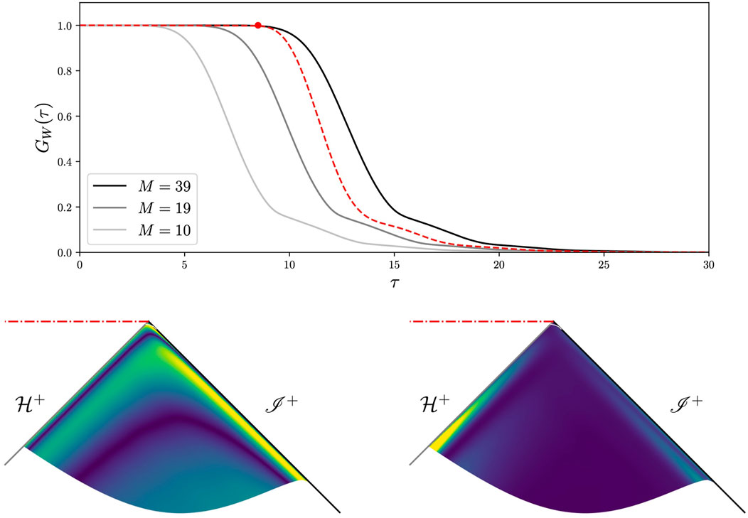
Figure 1. Energy growth curves and optimal perturbation for Schwarzschild $s=2,l=2$ Regge-Wheeler perturbations (figure taken from [22]). Top: $G_W$ for various $M=\dim (W)$ (solid curves), and the energy of an optimal perturbation of $M=39$ QNMs with ${\tau }_{\ast }=8.5$ (red-dash). Bottom: Modulus (left) and energy density (right) of the optimal perturbation in the conformal diagram of Schwarzschild. The energy is initially localised at ${\mathcal{H}}^{+}$ and ${\mathcal{I}}^{+}$, and then propagates along them until it starts dispersing and decaying at $\tau \simeq {\tau }_{\ast }$ (indicated by the white slice near $i^{+}$). The dash-dotted red line represents the curvature singularity.

Building on [22, 29] established the first case of transient energy growth in linear black hole perturbations considering RN-${\text{AdS}}_4$ black branes at chemical potential $\mu$ linearly perturbed by a complex scalar $\psi$ with charge $q$. The key difference here is that the total energy of the system does not correspond to the energy of $\psi$ alone. In particular, in the $q\to \infty$ limit suppressing backreaction to the metric, $E$ receives contributions from both the scalar, $\psi$, and the gauge field, $A$,

$E=E_{\psi }+E_F,(8)$

where $F=dA$, which are coupled to each other through $q$. Then, choosing $\Vert \cdot {\Vert }_{E_{\psi }}$ to construct optimal perturbations in the same fashion as before, $E_{\psi }$ was shown to exhibit significant transient growth before asymptotic decay via a transient form of superradiance–borrowing from the energy bath $E_F$ – in the modally stable regime.⁶ This is shown in the left panel of Figure 2, which displays $G_W$ and $E_{\psi }$ for an optimal perturbation with $M=10$ QNMs exhibiting transient growth. The first correction to the background gauge field energy, which appears at quadratic order in perturbations, $E_F^{(2)}$, takes negative values implying transfer of energy from $A$ to $\psi$, while the total energy $E=E_{\psi }+E_F^{(2)}$ can only decrease due to losses to the horizon. Empirically, it was observed that the peak of the growth curve increases with $M$ within the range of values considered. Note that this is not a special feature of the $q\to \infty$ limit, the finite $q$ case is also examined in [29] with same qualitative results.

Figure 2

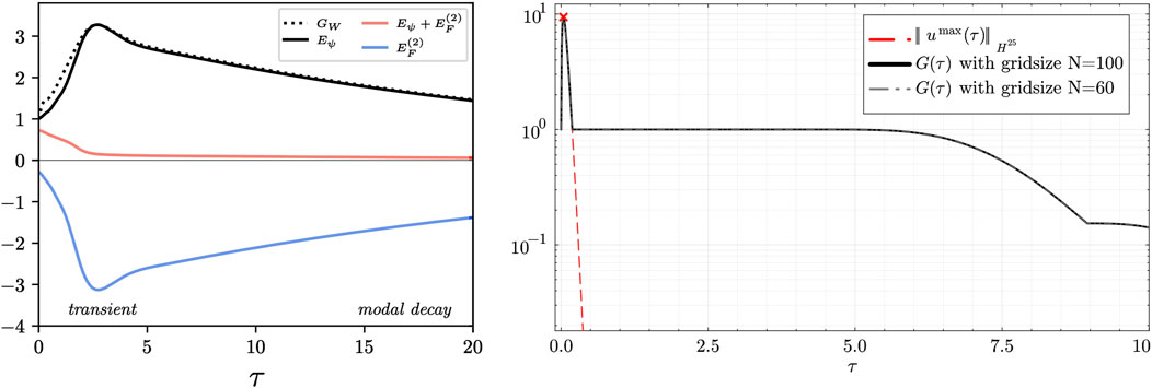
Figure 2. Left: optimal perturbation and energy growth curve $G_W(\tau )$ (black dash) for complex charged scalar QNMs of the RN-${\text{AdS}}_4$ black brane with $M=10$. $E_{\psi }$ (solid black curve) is shown to transiently grow before modally decaying at asymptotic time. The additional energy is borrowed from the energy bath $E_F$ via a transient form of superradiance, as can be seen from the first correction to $E_F$, $E_F^{(2)}$ (solid blue curve). The example shown corresponds to the probe limit $q\to \infty$ with $\mu q=3.9$, spatial momentum $\vec{k}=0$, with target time ${\tau }_{\ast }=2.7$. Figure taken from [29]. Right: growth curve $G$ and the norm of $u^{\text{max}}(\tau ,x)$ obtained by time-evolving the optimal perturbation $u_{\text{opt.}}({\tau }_{\ast }={\tau }_{\text{max}},x)$ in the Sobolev $H^{25}$ norm. A transient growth is observed and yields a peak at ${\tau }_{\text{max}}\approx \frac{1}{25}=0.04$, before a modal oscillatory decay. The growth curve $G$ is computed for two different resolutions $N=60$ (dashed gray curve) and $N=100$ (solid black curve), thus illustrating the convergence of the profile we observe on this panel. Figure taken from [26].

Transient behaviour has also been seen in Sobolev $H^p$ norms Equation 5 in [26] in the Pöschl-Teller toy model, corresponding to the Klein-Gordon equation in the static patch of de Sitter spacetime. Following a similar approach to [22, 29], optimal perturbations $u_{\text{opt.}}(0,x)$ were obtained using a ‘generalised’ singular value decomposition of the finite rank approximant of the evolution operator $e^{-i\mathcal{H}\tau }$, but this time without relying on a subspace of solutions $W$. For a target time ${\tau }_{\ast }$, these optimal perturbations maximise the Sobolev $H^p$ inner product such that ${⟨u_{\text{opt.}}({\tau }_{\ast },x),u_{\text{opt.}}({\tau }_{\ast },x)⟩}_{H^p}=G({\tau }_{\ast })$.

In the case of $H^0$ norm (corresponding to the energy norm), no transient growth is observed. Similar to [22], non-modal behaviour manifests itself as an initial transient plateau in $G$, followed by the expected modal decay, with a scalar field profile localised near the boundaries. However, unlike [22], the results are not convergent as the duration of the plateau scales as $\log N$ with the number of points $N$ used in the numerical approximation, further motivating the use of $H^p$ norms with $p>0$.

In the case of $H^p$ Sobolev norm with $p>0$, transient growth is observed. Specifically, one obtains an initial ‘peak’, which is followed by modal decay according to the lowest-lying QNM at late times; the right panel of Figure 2 exemplifies this behaviour for $p=25$, showing $G$ and ${⟨u_{\text{opt.}}({\tau }_{\ast },x),u_{\text{opt.}}({\tau }_{\ast },x)⟩}_{H^{25}}$ for ${\tau }_{\ast }={\tau }_{\text{max}}$ corresponding to the time of the peak. Note that $u_{\text{opt.}}({\tau }_{\ast },x)$ is an order-$p$ polynomial. The profile of the optimal perturbation $u_{\text{opt.}}(\tau ,x)$ is found to be numerically convergent and, importantly, it resides in the bulk of the geometry; this is different to the energy-norm case where the optimal perturbations was peaked near the boundaries. Applying the ‘Keldysh’ spectral decomposition scheme to $u_{\text{opt.}}(0,x)$ shows that most of the transient peak originates from the $(p+1)$-th pair of QNMs, ordered by decreasing $\mathfrak{I}\mathfrak{m}\omega$; note that the decay rate of these modes is $\frac{1}{p}$.

As the order $p$ of the $H^p$ Sobolev norm is increased, the peak in the growth curve increase as $G({\tau }_{\text{max}})={\max }_{\tau \ge 0}G(\tau )\sim p$ and moves to shorter timescales, ${\tau }_{\text{max}}\sim 1/p$. The scaling of ${\tau }_{\text{max}}$ is a result of the decay rate of the QNM giving rise to the majority of the transient peak mentioned above.

Lastly, it is illuminating to understand the existence of $H^p$-transient growth in the context of energy conservation. Specifically, the $H^p$-norm satisfies

$E\left[u\right]={⟨u,u⟩}_{H^p}-{\displaystyle \sum _{j=1}^p}{‖{\partial }_x^{j}u‖}_E^2,(9)$

where $E[u]$ is conserved up to boundary terms. In a way analogous to Equation 8, $H^p$-transient growth is permitted as a result of transfer of weight between the two terms in the right hand side of Equation 9.

Let us conclude this section with a comparison of the two methods discussed above: truncating the set of QNMs or using higher-derivative norms. Both approaches provide a way of regulating the UV and are equally easy to implement. The motivations for using them are different: in the former case the motivation was a physical truncation of the theory to low energy modes inspired by analogous constructions in hydrodynamics, while in the latter case the motivation was a consideration of regularity. The truncation method results in a finite dimensional Hilbert space which can be convenient to work with. The physical interpretation of the $H^p$-norm remains an open question.

4 Discussion

This short review summarises recent work on transient phenomena in black hole dynamics. The lack of normality of the evolution operator, emerging as a consequence of the dissipative nature of black hole spacetimes, results in the non-orthogonality of QNMs. This, in turn, allows for linear perturbations to exhibit non-modal behaviour (either in the form of transient growth or lack of decay) before eventually conforming to modal decay.

The existence of transients can be inferred from frequency-domain computations involving the pseudospectrum: the protrusion of pseudospectral contour lines in the unstable half plane indicates an unstable perturbed spectrum, and hence non-modal behaviour. In order to observe transient growth, the protrusion needs to be larger than the size of the external perturbation $ϵ$, giving rise to a Kreiss constant $\mathcal{K}>1$. This raises again the issue of the numerical convergence of the pseudospectrum as discussed in section 2, and motivates the exploration of the truncated-Hamiltonian pseudospectrum of [29].

Time-domain results exhibit striking qualitative similarities to the prototypical example of transient effects in the transition to turbulence in Navier-Stokes shear flows. Two particularly interesting questions that currently remain open relate to the non-linear evolution sourced by such initial data and the potential connection with the Aretakis instability.

Black hole QNMs have been a central focus of gravitational physics for over half a century, yet it remains striking that we still lack a full understanding of the consequences stemming from the absence of a spectral theorem in this context. This gap points to an exciting new direction in the field, suggesting that much remains to be uncovered. Particularly compelling questions include how much of the gravitational wave signal emanating from a binary merger can be attributed to linear transient dynamics, as well as the role of transients in strongly coupled systems, such as the quark-gluon plasma and high-temperature superconductors, via the AdS/CFT correspondence. Other arenas include analogue gravity systems, where fluid or optical setups mimic aspects of black hole spacetimes.

Author contributions

JB: Writing – review and editing, Writing – original draft. JC: Writing – review and editing, Writing – original draft. CP: Writing – original draft, Writing – review and editing. BW: Writing – review and editing, Writing – original draft.

Funding

The author(s) declare that financial support was received for the research and/or publication of this article. J.B. is supported by the project QuanTEdu-France 22-CMAS-0001. J.C. is supported by the Royal Society Research Grant RF\ERE \210267. C.P. is supported by a Royal Society – Research Ireland University Research Fellowship via grant URF\R1\211027. B.W. is supported by a Royal Society University Research Fellowship URF\R\231002 and in part by the STFC consolidated grant ST/T000775/1.

Acknowledgments

The authors would like to thank José Luis Jaramillo and Frans Pretorius for discussions.

Conflict of interest

The authors declare that the research was conducted in the absence of any commercial or financial relationships that could be construed as a potential conflict of interest.

Generative AI statement

The author(s) declare that no Generative AI was used in the creation of this manuscript.

Publisher’s note

All claims expressed in this article are solely those of the authors and do not necessarily represent those of their affiliated organizations, or those of the publisher, the editors and the reviewers. Any product that may be evaluated in this article, or claim that may be made by its manufacturer, is not guaranteed or endorsed by the publisher.

Footnotes

¹Second order QNMs, usually referred to as QQNMs, have also been constructed recently [3, 4].

²With respect to standard choices of inner product. See [10–13] for the construction of QNM orthogonality relations in other products.

³See also [21] for a related study of extreme compact objects, where a Kreiss constant consistent with $K(\mathcal{H})=1$ was obtained numerically by computing the ratio of the pseudospectral abscissa ${\alpha }_{ϵ}(\mathcal{H})/ϵ$ in the limit $ϵ\to \infty$.

⁴Note that [23] reports transient growth in the context of Kaluza-Klein black holes in Gauss-Bonnet gravity. However, the system studied in [23] is conservative up to boundary terms and (3.19) there can be written as a total derivative. As such, the reported result on transient growth is incorrect.

⁵Note that this is different to the corresponding inner product used in [24].

⁶In AdS/CFT, this model is known as the holographic superconductor [36–38], and it is linearly unstable for $T<T_c$ (or equivalently $\mu >{\mu }_c$) corresponding to the superconducting phase.

References

1. Berti E, Cardoso V, Starinets AO. Quasinormal modes of black holes and black branes. Class Quant Grav (2009) 26:163001. doi:10.1088/0264-9381/26/16/163001

CrossRef Full Text | Google Scholar

2. Konoplya RA, Zhidenko A. Quasinormal modes of black holes: from astrophysics to string theory. Rev Mod Phys (2011) 83:793–836. doi:10.1103/RevModPhys.83.793

CrossRef Full Text | Google Scholar

3. Lagos M, Hui L. Generation and propagation of nonlinear quasinormal modes of a Schwarzschild black hole. Phys Rev D (2023) 107:044040. doi:10.1103/PhysRevD.107.044040

CrossRef Full Text | Google Scholar

4. Pantelidou C, Withers B. Thermal three-point functions from holographic Schwinger-Keldysh contours. JHEP (2023) 04:050. doi:10.1007/JHEP04(2023)050

CrossRef Full Text | Google Scholar

5. Policastro G, Son DT, Starinets AO. The Shear viscosity of strongly coupled N=4 supersymmetric Yang-Mills plasma. Phys Rev Lett (2001) 87:081601. doi:10.1103/PhysRevLett.87.081601

PubMed Abstract | CrossRef Full Text | Google Scholar

6. Kovtun PK, Starinets AO. Quasinormal modes and holography. Phys Rev D (2005) 72:086009. doi:10.1103/PhysRevD.72.086009

CrossRef Full Text | Google Scholar

7. Baibhav V, Cheung MHY, Berti E, Cardoso V, Carullo G, Cotesta R, et al. Agnostic black hole spectroscopy: quasinormal mode content of numerical relativity waveforms and limits of validity of linear perturbation theory. Phys Rev D (2023) 108:104020. doi:10.1103/PhysRevD.108.104020

CrossRef Full Text | Google Scholar

8. York JW. Dynamical origin of black hole radiance. Phys Rev D (1983) 28:2929–45. doi:10.1103/PhysRevD.28.2929

CrossRef Full Text | Google Scholar

9. Hintz P, Vasy A. Analysis of linear waves near the Cauchy horizon of cosmological black holes. J Math Phys (2017) 58:081509. doi:10.1063/1.4996575

CrossRef Full Text | Google Scholar

10. Jafferis DL, Lupsasca A, Lysov V, Ng GS, Strominger A. Quasinormal quantization in de Sitter spacetime. JHEP (2015) 1:004. doi:10.1007/JHEP01(2015)004

CrossRef Full Text | Google Scholar

11. Green SR, Hollands S, Sberna L, Toomani V, Zimmerman P. Conserved currents for a Kerr black hole and orthogonality of quasinormal modes. Phys Rev D (2023) 107:064030. doi:10.1103/PhysRevD.107.064030

CrossRef Full Text | Google Scholar

12. London LT. A radial scalar product for Kerr quasinormal modes. arXiv:2312.17678 (2023).

Google Scholar

13. Arnaudo P, Carballo J, Withers B. QNM orthogonality relations for AdS black holes. arXiv:2505.04696 (2025).

Google Scholar

14. Krejcirik D, Siegl P, Tater M, Viola J. Pseudospectra in non-Hermitian quantum mechanics. J Math Phys (2015) 56:103513. doi:10.1063/1.4934378

CrossRef Full Text | Google Scholar

15. Trefethen L, Embree M. Spectra and pseudospectra: the behavior of nonnormal matrices and operators. Princeton University Press (2005).

Google Scholar

16. Gasperin E, Jaramillo JL. Energy scales and black hole pseudospectra: the structural role of the scalar product. Class Quant Grav (2022) 39:115010. doi:10.1088/1361-6382/ac5054

CrossRef Full Text | Google Scholar

17. Jaramillo JL, Panosso Macedo R, Al Sheikh L. Pseudospectrum and black hole quasinormal mode instability. Phys Rev X (2021) 11:031003. doi:10.1103/PhysRevX.11.031003

CrossRef Full Text | Google Scholar

18. Nollert HP, Price RH. Quantifying excitations of quasinormal mode systems. J Math Phys (1999) 40:980–1010. doi:10.1063/1.532698

CrossRef Full Text | Google Scholar

19. Nollert HP. About the significance of quasinormal modes of black holes. Phys Rev D (1996) 53:4397–402. doi:10.1103/PhysRevD.53.4397

PubMed Abstract | CrossRef Full Text | Google Scholar

20. Jaramillo JL. Pseudospectrum and binary black hole merger transients. Class Quant Grav (2022) 39:217002. doi:10.1088/1361-6382/ac8ddc

CrossRef Full Text | Google Scholar

21. Boyanov V, Destounis K, Panosso Macedo R, Cardoso V, Jaramillo JL. Pseudospectrum of horizonless compact objects: a bootstrap instability mechanism. Phys Rev D (2023) 107:064012. doi:10.1103/PhysRevD.107.064012

CrossRef Full Text | Google Scholar

22. Carballo J, Withers B. Transient dynamics of quasinormal mode sums. JHEP (2024) 10:084. doi:10.1007/JHEP10(2024)084

CrossRef Full Text | Google Scholar

23. Chen JN, Wu LB, Guo ZK. The pseudospectrum and transient of Kaluza–Klein black holes in Einstein–Gauss–Bonnet gravity. Class Quant Grav (2024) 41:235015. doi:10.1088/1361-6382/ad89a1

CrossRef Full Text | Google Scholar

24. Boyanov V, Cardoso V, Destounis K, Jaramillo JL, Macedo RP. Structural aspects of the anti–de sitter black hole pseudospectrum. Phys Rev D (2024) 109:064068. doi:10.1103/PhysRevD.109.064068

CrossRef Full Text | Google Scholar

25. Warnick C. Stability of de sitter quasinormal mode spectra (2024) 19850. arXiv:2407.

Google Scholar

26. Besson J, Jaramillo JL. Quasi-normal mode expansions of black hole perturbations: a hyperboloidal Keldysh’s approach. Gen Relativ Gravit (2025) 57:110. doi:10.1007/s10714-025-03438-6

CrossRef Full Text | Google Scholar

27. Warnick CM. On quasinormal modes of asymptotically anti-de Sitter black holes. Commun Math Phys (2015) 333:959–1035. doi:10.1007/s00220-014-2171-1

CrossRef Full Text | Google Scholar

28. Bizoń P, Chmaj T, Mach P. A toy model of hyperboloidal approach to quasinormal modes. Acta Phys Polon B (2020) 51:1007. doi:10.5506/APhysPolB.51.1007

CrossRef Full Text | Google Scholar

29. Carballo J, Pantelidou C, Withers B. Non-modal effects in black hole perturbation theory: transient Superradiance. arXiv:2503. 05871. (2025).

Google Scholar

30. Reddy SC, Schmid PJ, Henningson DS. Pseudospectra of the orr-sommerfeld operator. SIAM J Appl Mathematics (1993) 53:15–47. doi:10.1137/0153002

CrossRef Full Text | Google Scholar

31. Gustavsson LH. Energy growth of three-dimensional disturbances in plane Poiseuille flow. J Fluid Mech (1991) 224:241–60. doi:10.1017/S002211209100174X

CrossRef Full Text | Google Scholar

32. Henningson DS, Lundbladh A, Johansson AV. A mechanism for bypass transition from localized disturbances in wall-bounded shear flows. J Fluid Mech (1993) 250:169–207. doi:10.1017/S0022112093001429

CrossRef Full Text | Google Scholar

33. Butler KM, Farrell BF. Three-dimensional optimal perturbations in viscous shear flow. Phys Fluids A: Fluid Dyn (1992) 4:1637–50. doi:10.1063/1.858386

CrossRef Full Text | Google Scholar

34. Reddy SC, Henningson DS. Energy growth in viscous channel flows. J Fluid Mech (1993) 252:209–38. doi:10.1017/S0022112093003738

CrossRef Full Text | Google Scholar

35. Trefethen LN, Trefethen AE, Reddy SC, Driscoll TA. Hydrodynamic stability without eigenvalues. Science (1993) 261:578–84. doi:10.1126/science.261.5121.578

PubMed Abstract | CrossRef Full Text | Google Scholar

36. Gubser SS. Breaking an Abelian gauge symmetry near a black hole horizon. Phys Rev D (2008) 78, 065034. doi:10.1103/PhysRevD.78.065034

CrossRef Full Text | Google Scholar

37. Hartnoll SA, Herzog CP, Horowitz GT. Building a holographic superconductor. Phys Rev Lett (2008) 101, 031601. doi:10.1103/PhysRevLett.101.031601

PubMed Abstract | CrossRef Full Text | Google Scholar

38. Hartnoll SA, Herzog CP, Horowitz GT. Holographic superconductors. JHEP (2008) 12, 015. doi:10.1088/1126-6708/2008/12/015

CrossRef Full Text | Google Scholar