 Jean-Michel Tucny
 Mihir Durve
 Sauro Succi
- 1Department of Civil, Computer Science, and Aeronautical Technologies Engineering, Università degli Studi Roma Tre, Rome, Italy
- 2Center for Life Nano- & Neuro-Science, Italian Institute of Technology (IIT), Rome, Italy
The rise of deep learning challenges the longstanding scientific ideal of insight—the human ability to understand phenomena by uncovering underlying mechanisms. From a physics perspective, we examine this tension through a case study: a physics-informed neural network (PINN) trained on rarefied gas dynamics governed by the Boltzmann equation. Despite strong physical constraints and a system with clear mechanistic structure, the trained network’s weight distributions remain close to Gaussian, showing no coarse-grained signature of the underlying physics. This result contrasts with theoretical expectations that such networks might retain structural features akin to discrete dynamical systems. We argue that high predictive accuracy does not imply interpretable internal representations and that explainability in physics-informed AI may not always be achievable—or necessary. These findings highlight a growing divergence between models that predict well and those that offer insight.
1 Introduction
Recent advances in machine learning (ML), particularly through large language models (LLMs), have dramatically reshaped both science and society. These models now routinely tackle problems previously thought to be beyond reach, ranging from natural language understanding and protein folding to autonomous systems and symbolic reasoning [1–3]. Such progress introduces a fundamentally different approach to scientific discovery—one based not on physical insight into underlying mechanisms, but on data-driven optimization through a dense web of parameters. While physics-informed constraints can improve convergence [4], the learning process itself often remains opaque.
It no longer appears tenable to dismiss ML as a “glorified interpolator” or LLMs as “stochastic parrots” [5]. Instead, ML is beginning to challenge the very role of mechanistic understanding—or what has traditionally been called Insight—in scientific modeling. This tension raises the possibility of an ”End of Insight” (EoI), a term coined by Strogatz [6], referring to the notion that certain scientific challenges may resist explanation in terms of simple governing principles, especially when they involve multiple interacting processes across vastly different scales in space and time.
This prospect is sad and perilous but plausible. Insight, as shaped by centuries of theory-driven physics, may not scale gracefully to problems such as epidemics, climate dynamics, or non-equilibrium statistical systems. ML, unconcerned with interpretability, may allow us to push the frontiers of knowledge in such domains—but without the perk of Insight and the intimate pleasure of ”finding things out”. This should not distract us from the fact that ML is still subject to a number of major limitations, especially when paired with the rising energy cost of training ever-larger models, a trajectory that raises concerns about sustainability and rapidly diminishing returns [7].
In this paper, we contribute to this discussion through a focused case study: a physics-informed neural network (PINN) trained on a rarefied gas flow governed by the Boltzmann equation. The problem is highly structured, well understood, and modeled using both mechanistic equations and direct numerical simulation. Given these features—and the close connection between machine learning and discrete dynamical systems—we explore whether the network’s parameters retain coarse signatures of the underlying physics. Rather than aiming to resolve interpretability, we use this controlled setting to test assumptions about what structured learning might look like when physical constraints are strongly present.
2 The basic ML procedure
The basic idea of ML lies in approximating a
where
where
2.1 Taming complexity
It is often claimed that, with enough data, ML can approximate virtually any target, whence the alleged demise of the scientific method [9, 10]. Put down in such bombastic terms, the idea is readily debunked by general considerations on the physics of complex systems, see for instance [11, 12]. Yet, ML does show remarkable proficiency in handling problems resistant to conventional modeling.
To understand why, we briefly examine the three main boosters of Complexity: Nonlinearity, Nonlocality and Hyper-Dimensionality.
2.1.1 Nonlinearity
Nonlinear systems exhibit two distinguishing and far-reaching features: i) they do not respond proportionally to input, and ii) they transfer energy (information) across scales. This makes them erratic and hard to predict, but also capable of emergent phenomena—complex behavior arising from simple rules, biology being a goldmine of such instances. While physics has developed mathematical tools to handle nonlinearity, these are often overwhelmed when couplings become too strong across vast scales, with weather forecasting being a prominent example. ML can definitely help such methods stretch their limits. However, at present, there is no clear evidence that it can systematically outperform them, especially when precision is in high demand, as is usually the case for scientific applications [13].
2.1.2 Nonlocality
In nonlocal systems, local behavior depends on distant states, often via long-range couplings. Although this interaction usually decays with the distance between the two regions, it cannot be ignored, no matter how far the interacting components are. A typical example from physics is classical gravitation, which is controlled by a potential decaying with the inverse power of the distance. The peculiarity of these systems is that they hardly reach a state of dynamic order known as ”local equilibrium”, usually controlled by a subset of ”slow” variables living in a lower-dimensional manifold. Local equilibrium is the result of a neat scale separation between slow and fast variables, a feature which greatly simplifies the dynamics. Dynamics is notoriously much harder to capture than statistics and this is the reason why statistical physics is so effective in describing complex systems. With nonlocality in play, even statistical mechanics may remain hard to capture because of the aforementioned lack of scale separation between fast and slow modes. ML has shown promise in capturing such structures, particularly in identifying latent manifolds, though it remains an empirical rather than systematic approach [14].
2.1.3 Hyper-dimensionality
High-dimensional systems often suffer from the so-called curse of dimensionality (CoD), where the state space grows exponentially with the number of variables. Yet the real difficulty is subtler: due to nonlinearities, heterogeneities, and other structural constraints, important phenomena typically occur in sparse, low-volume regions of this vast space—what we might call the ”golden nuggets”. Locating these nuggets is exponentially hard, and this is where ML excels [15].
A deep neural network (DNN) with width
Modern ML applications such as DeepFold and LLMs now use up to 100 billion parameters—roughly the number of neurons in the human brain. But unlike our 20 W cerebral hardware, these models can require gigawatt-scale resources. It is estimated that next-generation chatbots will approach the gigawatt power demand, more than most existing power plants. This unveils the fundamental tension: ML systems trade Insight for brute-force optimization, and with it comes massive energy cost. The question is whether the End of Insight also implies the end of the energetic resources of planet Earth, in which case one has probably to think twice before endorsing the ”bigger is better” route undertaken by Big Tech companies [16].
The academic community is exploring ways to mitigate this, often with limited means. In the next section, we offer one such contribution: reframing ML as a class of discrete dynamical systems, namely, generalized diffusion-advection processes. This analogy allows weights to acquire physical meaning, potentially enabling more interpretable and energy-efficient learning strategies [17].
Let us describe the idea in more detail.
3 Machine learning and discrete dynamical systems
In a recent paper [17], the ML procedure was formally reinterpreted as a discrete dynamical system in relaxation form: more precisely, as a time-discretized neural integro-equation (NIDE) of the form shown in Equation 5:
where
The mapping
where
The procedure is quite transparent, both conceptually and mathematically: the solution
A simple Euler time marching of the Equation 5, as combined with a suitable discretization of the ”space” variable
where
Clearly, the result is highly dependent on the structure of the convolution kernel
The argument can be easily extended to more general PDEs, including strong inhomogeneities and nonlinearities, which could easily be implemented by convoluting local nonlinear combinations of the signal, as shown in Equation 9:
where
For instance, by truncating the integral to the second moment, we would obtain
4 Inspecting the weights of a PINN application to rarefied gas dynamics
The preceding considerations suggest that analyzing the weights of a trained network might offer insight into its internal logic, particularly when the problem is governed by a well-understood physical model. Let us test the idea by means of a concrete application. Recently, we trained a physics-informed neural network (PINN) on a body-force-driven rarefied gas flow through a 2D periodic array of cylinders in the laminar, isothermal and weakly compressible limit [19]. This problem has a well-defined structure governed by the Boltzmann equation (BE).
A key parameter in rarefied gas dynamics is the Knudsen number
Motivated by these challenges, we designed a neural network that takes as input the spatial coordinates
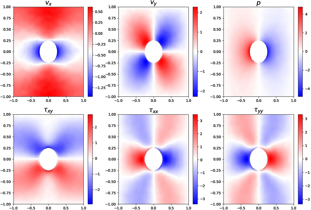
Figure 1. Normalized macroscopic fields predicted by the PINN for
The network consists of a Fourier layer to impose periodic boundary conditions [20, 21], followed by nine hidden layers of 100 neurons with
Additional pre-processing was required to ensure convergence. Pressure fields were debiased across the Knudsen range due to their artificial variation stemming from how Kn was numerically set. Likewise, velocity vectors lost orientation under normalization, which was necessary to stabilize training but severs their physical directional meaning. Finally, L1L2 regularization was applied to promote smoothness and broad participation across weights rather than sparse activation.
These design choices—though effective for learning—blur direct links between physical content and internal network representations. The basic question we pursue is whether, despite these compromises, the trained network retains any recognizable physical structure. Before discussing the results, let us first show that our problem does exhibit the three key properties we described as where neural networks should excel. To this purpose, let us recall basic facts about the Boltzmann equation (BE).
4.1 The Boltzmann equation
This equation describes the dynamics of the probability density function
The left hand side represents the free streaming of the molecules, while the right hand encodes molecular collisions via a quadratic integral in velocity space involving the product
where
This structure embeds all three complexity boosters: nonlinearity via the quadratic collision term, nonlocality through the transport of information across space and velocity scales, and high dimensionality due to its formulation in six-dimensional phase space (plus time). While
Even more relevant to macroscopic observables, integration of the BE over velocities yields transport equations that are simultaneously nonlinear and nonlocal in physical space, such as the familiar convective term
5 Learning the Boltzmann solutions via PINNs
The PINN described above is trained on numerical data from Direct Simulation Monte Carlo of the Boltzmann equation [26]. Given the problem’s high physical structure and the inclusion of physics-informed loss terms, one might expect this to manifest in structured, interpretable weight patterns. However, as shown in Figure 2, the distribution of weights in the deepest layer closely resembles a zero-mean Gaussian. While small but statistically significant departures from normality are detected—excess kurtosis between −0.65 and −0.5, Kolmogorov–Smirnov (KS) distances between 0.015 and 0.03—these deviations do not amount to the emergence of any discernible physical structure. No clear trace of the governing equations appears to persist in the weight statistics.
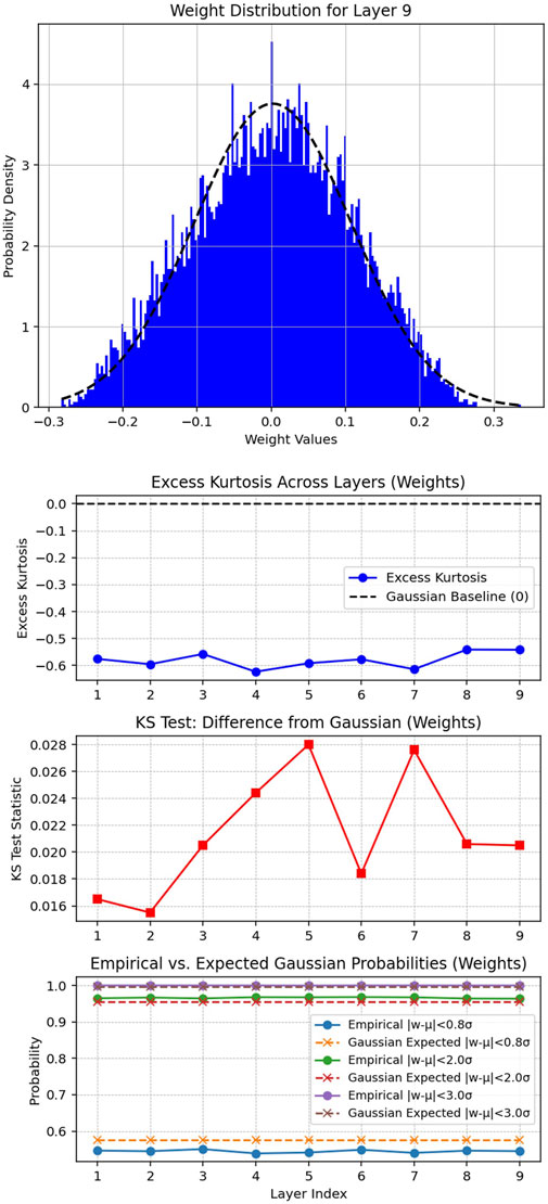
Figure 2. Distribution of weights in the deepest layer. The PDF is overlaid with a standard Gaussian. The excess kurtosis and KS statistical analysis indicates a weak, but statistically significant departure from normality.
One possible explanation for this mismatch lies in the conceptual assumptions behind the analogy between machine learning and discrete dynamical systems. Such analogies typically rely on the presence of an ordered metric structure among discrete coordinates
7 Tentative conclusions and outlook
The analysis of a PINN trained on a rarefied gas flow problem reveals a striking disconnect between the physical structure of the governing Boltzmann equation and the internal organization of the network. Despite being constrained by physics-informed losses, the network’s weights resemble near-Gaussian distributions with no evident trace of the underlying integro-differential operator. This supports the view that machine learning and traditional simulation can offer functionally equivalent yet epistemologically distinct routes to the same solution.
That such a disconnect emerges even for a moderately complex and well-understood problem raises a deeper question: beyond a certain threshold of complexity, might Insight—as traditionally pursued in physics—become practically inaccessible? If so, the role of explainability must be rethought, not as a universal standard, but as a domain-dependent aspiration.
This need not be cause for alarm. A lack of interpretable structure at the parameter level does not imply that ML is unscientific—but it does suggest that physical knowledge and machine-learned representations follow fundamentally different logics. Bridging them may require new tools, not just to improve interpretability, but to reframe what interpretability itself should mean in AI-augmented science.
Data availability statement
The raw data supporting the conclusions of this article will be made available by the authors, upon reasonable request.
Author contributions
J-MT: Data curation, Formal Analysis, Funding acquisition, Investigation, Methodology, Resources, Software, Validation, Visualization, Writing – original draft. MD: Formal Analysis, Funding acquisition, Investigation, Methodology, Resources, Software, Validation, Writing – review and editing. SS: Conceptualization, Data curation, Formal Analysis, Funding acquisition, Investigation, Methodology, Project administration, Resources, Supervision, Validation, Writing – original draft.
Funding
The author(s) declare that financial support was received for the research and/or publication of this article. SS is grateful to SISSA for financial support under the “Collaborations of Excellence” initiative and to the Simons Foundation for supporting several enriching visits. He also wishes to acknowledge many enlightening discussions with PV Coveney, A. Laio, D. Spergel and S. Strogatz. JMT is grateful to the FRQNT “Fonds de recherche du Québec - Nature et technologies (FRQNT)” for financial support (Research Scholarship No. 357484). SS and MD gratefully acknowledge funding by the European Union (EU) under the Horizon Europe research and innovation programme, EIC Pathfinder - grant No. 101187428 (iNSIGHT) and from the European Research Council ERC-PoC2 grant No. 101187935 (LBFAST).
Conflict of interest
The authors declare that the research was conducted in the absence of any commercial or financial relationships that could be construed as a potential conflict of interest.
Generative AI statement
The author(s) declare that Generative AI was used in the creation of this manuscript. The large language model ChatGPT-4o was used to assist in improving the clarity and conciseness of the English in this manuscript. The authors take full responsibility for the content and interpretations presented.
Any alternative text (alt text) provided alongside figures in this article has been generated by Frontiers with the support of artificial intelligence and reasonable efforts have been made to ensure accuracy, including review by the authors wherever possible. If you identify any issues, please contact us.
Publisher’s note
All claims expressed in this article are solely those of the authors and do not necessarily represent those of their affiliated organizations, or those of the publisher, the editors and the reviewers. Any product that may be evaluated in this article, or claim that may be made by its manufacturer, is not guaranteed or endorsed by the publisher.
References
1. Vaswani A, Shazeer N, Parmar N, Uszkoreit J, Jones L, Gomez AN, et al. Attention is all you need. Adv Neural Inf Process Syst (2017) 30.
2. Jumper J, Evans R, Pritzel A, Green T, Figurnov M, Ronneberger O, et al. Highly accurate protein structure prediction with alphafold. nature (2021) 596:583–9. doi:10.1038/s41586-021-03819-2
4. Cai S, Mao Z, Wang Z, Yin M, Karniadakis GE. Physics-informed neural networks (pinns) for fluid mechanics: a review. Acta Mechanica Sinica (2021) 37:1727–38. doi:10.1007/s10409-021-01148-1
5. Bender EM, Gebru T, McMillan-Major A, Shmitchell S. On the dangers of stochastic parrots: can language models be too big? In: Proceedings of the 2021 ACM conference on fairness, accountability, and transparency, FAccT 21. New York, NY, USA: Association for Computing Machinery (2021). p. 610–23.
6. Strogatz S. The end of insight. In: What is your dangerous idea? today’s leading thinkers on the unthinkable. New York, NW: Simon & Schuster (2007).
7. Succi S. Chatbots and zero sales resistence. Front Phys (2024) 12:1484701. doi:10.3389/fphy.2024.1484701
9. Anderson C. The end of theory: the data deluge makes the scientific method obsolete. Wired Mag (2008) 16:16.
10. Hasperué W. The master algorithm: how the quest for the ultimate learning machine will remake our world. J Computer Sci & Technology (2015) 15.
11. Coveney PV, Dougherty ER, Highfield RR. Big data need big theory too. Philosophical Trans R Soc A: Math Phys Eng Sci (2016) 374:20160153. doi:10.1098/rsta.2016.0153
12. Succi S, Coveney PV. Big data: the end of the scientific method? Philosophical Trans R Soc A (2019) 377:20180145. doi:10.1098/rsta.2018.0145
13. Coveney PV, Highfield R. Artificial intelligence must be made more scientific. J Chem Inf Model (2024) 64:5739–41. doi:10.1021/acs.jcim.4c01091
14. Strogatz SH. Nonlinear dynamics and chaos: with applications to physics, biology, chemistry, and engineering. Chapman and Hall/CRC (2024).
15. Poggio T, Mhaskar H, Rosasco L, Miranda B, Liao Q. Why and when can deep-but not shallow-networks avoid the curse of dimensionality: a review. Int J Automation Comput (2017) 14:503–19. doi:10.1007/s11633-017-1054-2
16. Hassabis D, Kumaran D, Summerfield C, Botvinick M. Neuroscience-inspired artificial intelligence. Neuron (2017) 95:245–58. doi:10.1016/j.neuron.2017.06.011
17. Succi S. A note on the physical interpretation of neural pde’s. arXiv preprint arXiv:2502.06739. (2025). doi:10.48550/arXiv.2502.06739
18. Han J, Jentzen A, E W. Solving high-dimensional partial differential equations using deep learning. Proc Natl Acad Sci (2018) 115:8505–10. doi:10.1073/pnas.1718942115
19. Tucny J-M, Lauricella M, Durve M, Guglielmo G, Montessori A, Succi S. Physics-informed neural networks for microflows: rarefied gas dynamics in cylinder arrays. J Comput Sci (2025) 87:102575. doi:10.1016/j.jocs.2025.102575
20. Dong S, Ni N. A method for representing periodic functions and enforcing exactly periodic boundary conditions with deep neural networks. J Comput Phys (2021) 435:110242. doi:10.1016/j.jcp.2021.110242
21. Lu L, Pestourie R, Yao W, Wang Z, Verdugo F, Johnson SG. Physics-informed neural networks with hard constraints for inverse design. SIAM J Scientific Comput (2021) 43:B1105–32. doi:10.1137/21m1397908
22. Succi S. The lattice boltzmann equation: for complex states of flowing matter. Oxford: Oxford University Press (2018).
23. Calì A, Succi S, Cancelliere A, Benzi R, Gramignani M. Diffusion and hydrodynamic dispersion with the lattice boltzmann method. Phys Rev A (1992) 45:5771–4. doi:10.1103/physreva.45.5771
24. Rybicki FJ, Melchionna S, Mitsouras D, Coskun AU, Whitmore AG, Steigner M, et al. Prediction of coronary artery plaque progression and potential rupture from 320-detector row prospectively ecg-gated single heart beat ct angiography: lattice boltzmann evaluation of endothelial shear stress. The Int J Cardiovasc Imaging (2009) 25:289–99. doi:10.1007/s10554-008-9418-x
25. D’Orazio A, Succi S. Boundary conditions for thermal lattice boltzmann simulations. In: International conference on computational science. Springer (2003). p. 977–86.
Keywords: explainable artificial intelligence (XAI), physics-informed neural networks (pinns), interpretability, Boltzmann equation, rarefied gas dynamics, machine learning, random matrix theory
Citation: Tucny J-M, Durve M and Succi S (2025) Is the end of insight in sight?. Front. Phys. 13:1641727. doi: 10.3389/fphy.2025.1641727
Received: 05 June 2025; Accepted: 16 September 2025;
Published: 08 October 2025.
Edited by:
Alex Hansen, NTNU, NorwayReviewed by:
Raffaela Cabriolu, Norwegian University of Science and Technology, NorwayCopyright © 2025 Tucny, Durve and Succi. This is an open-access article distributed under the terms of the Creative Commons Attribution License (CC BY). The use, distribution or reproduction in other forums is permitted, provided the original author(s) and the copyright owner(s) are credited and that the original publication in this journal is cited, in accordance with accepted academic practice. No use, distribution or reproduction is permitted which does not comply with these terms.
*Correspondence: Jean-Michel Tucny, amVhbm1pY2hlbC50dWNueUB1bmlyb21hMy5pdA==