A TPS-based numerical method for simulating the non-linear diffusion logistic population model

The Fisher–Kolmogorov–Petrovsky–Piskunov equation is a diffusive logistic model for the population density of an invasive species. This paper presents a one-level numerical simulation of the non-linear diffusion logistic population model using the thin plate spline (TPS) radial basis function (RBF) collocation method. Based on the combination of time and space variables, the time–space points are constructed. During the collocation procedure, the non-uniform point distribution case is considered for comparison with the traditional uniform point distribution case. Numerical examples show that the one-level TPS-RBF collocation method avoids the complexities of mesh generation and re-meshing. We can conclude that non-uniform point distributions yield higher accuracy in simulating the non-linear diffusion logistic population model than uniform distributions, especially with increased collocation point density. The efficiency, accuracy, and stability of the proposed method are demonstrated through numerical experiments.

1 Introduction

The Fisher–Kolmogorov–Petrovsky–Piskunov (Fisher–KPP) equation, which is also termed the reaction–diffusion equation, is an important model in population biology that characterizes the wavefront propagation dynamics of advantageous genes in spatially extended systems. This equation can describe the spatial diffusion of invasive species, and it is typically formulated as [1, 2]

$u_t=\alpha u_{xx}+\beta u\left(1-\frac{u}{k}\right),a<x<b,t>0,(1)$

where $u$ is the population density reflecting the distribution intensity of biological populations, $t$ is time, and $x$ is the space variable. $\alpha$ represents the diffusion coefficient that quantifies the random migration rate of individuals in a population in the given space. It is consistent with the physical meaning of the diffusion coefficient in Fick’s second law. $\beta$ is the intrinsic growth rate, which characterizes the maximum proliferation rate of a population without resource constraints. $k$ is the environmental carrying capacity that describes the maximum sustainable population density that an ecosystem can sustain, reflecting the saturation effect of resource constraints on population growth. The diffusion term $\alpha u_{xx}$ describes the diffusion process of a population in space, and it is derived from the statistical law of individual random motion. The reaction term $\beta u\left(1-\frac{u}{k}\right)$ reflects the growth and competition of the population, where $1-\frac{u}{k}$ represents the density constraint effect caused by resource constraints.

As is known to all, solutions to partial differential equations (PDEs) should be accompanied with initial/boundary conditions. The corresponding initial and boundary conditions for governing Equation 1 are usually given as

$u\left(x,0\right)=u_1\left(x\right),x=a,\text{and}x=b,(2)$

$u\left(x,t\right)=u_2\left(x,t\right),t>0.(3)$

Here, $u_1\left(x\right)$ and $u_2\left(x,t\right)$ are prescribed smooth functions.

Due to the inherent non-linear dynamics and wavefront propagation challenges in the Fisher–KPP equation, numerical approaches are considered a critical framework for constructing stable approximations to its solutions rather than analytical solutions [3–5]. [6] used the Adomian decomposition method to construct an approximate solution of the generalized Fisher–KPP equation. [7] revisited traveling wave solutions of the Fisher–KPP model and showed that these results provide new insight into traveling wave solutions of the Fisher–Stefan model and the spreading–extinction dichotomy. The general construction of the Cauchy problem solution for the Fisher–KPP equation is described in terms of semiclassical asymptotics based on the complex WKB–Maslov method by [8]. [9] presented an unconditionally stable positivity-preserving numerical method for the Fisher–KPP equation. [10] investigated the bounds on the critical times for the general Fisher–KPP equation. Under conditions of weak diffusion, [11] used numerical methods to compare the processes of spatiotemporal pattern formation in a nonlocal population model described by a 1-D generalized Fisher–KPP equation with nonlocal competitive losses. [12] established results using a combination of high-accuracy numerical simulations to investigate the non-vanishing sharp-fronted traveling wave solutions of the Fisher–KPP model. [13] proposed modeling the growth of Candida auris with a computationally randomized Fisher–KPP partial differential equation. [14] proposed an approximate solution based on 2D shifted Legendre polynomials to solve the non-linear stochastic Fisher–KPP equation with space uniform white noise for the same. [15] used an asymptotic approach to investigate moving singularities of the forced Fisher–KPP equation. [16] explored the numerical solution of the Fisher–KPP equation through two meshless methods. [17] proposed an approximate solution based on 2D shifted Legendre polynomials to solve the non-linear Fisher–KPP model under nonlocal competition. The positivity-preserving and unconditionally stable numerical scheme for the 3D modified Fisher–KPP equation was demonstrated by [18].

Although existing research studies have explored meshless approaches for the Fisher–KPP equation, these implementations typically require a two-level numerical procedure where the meshless method must be coupled with extra numerical techniques to handle time-dependent temporal derivatives in the governing equation. To circumvent the two-level procedure, we introduce a one-level meshless approach to solve the Fisher–KPP equation, where the time-dependent temporal derivative is reformulated as a spatial term through a unified space–time framework. Since the thin plate spline radial basis function (TPS-RBF) kernel functions have good mathematical properties, they facilitate theoretical analysis and calculation. The TPS-RBF has been widely used in various applications, including image registration, shape analysis, and numerical solution of PDEs [19–21]. In this paper, we focus on the TPS-RBF-based collocation method for the numerical simulation of the spatial diffusion of invasive species governed by the Fisher–KPP equation. The methodology of the proposed one-level meshless method is presented in Section 2. Several numerical examples are provided in Section 3 to show the efficiency, accuracy, and stability of the proposed method. Some concluding remarks with future directions are provided in Section 4.

2 Methodology

2.1 Space–time TPS-RBF

The TPS-RBF is one of the traditional RBFs based on distance measurement. Compared with the multiquadrics and Gaussian RBF [22, 23], it is parameter-free. It also has the advantage of high flexibility, can adapt to complex data distributions, and performs particularly well when dealing with non-linear data.

For 2D problems, it is defined as

$\phi \left(r\right)=r^2\log r.(4)$

Here, $r=‖X_i-X_j‖$ is the Euclidean distance between the two points $X_i=\left(x_i,y_i\right)$ and $X_j=\left(x_j,y_j\right)$.

There is only one space variable $x$ in F–KPP Equation 1. To facilitate the numerical procedure, the time variable $t$ is “equally” considered as a new space variable. Hence, one can obtain a new space–time point $\left(x,t\right)$. To avoid confusion with Equation 4, the corresponding space–time RBFs can be expressed as

$\varphi \left(\overline{r}\right)={\overline{r}}^2\log \overline{r},(5)$

where $\overline{r}=\sqrt{{\left(x_i-x_j\right)}^2+{\left(t_i-t_j\right)}^2}$ is the distance between the points ${\overline{X}}_i=\left(x_i,t_i\right)$ and ${\overline{X}}_j=\left(x_j,t_j\right)$.

2.2 Collocation method

The collocation method is a numerical technique for solving PDEs by enforcing the governing equation at a set of discrete collocation points [24, 25]. In the context of RBF collocation, the unknown solution is approximated as a linear combination of RBFs centered at the collocation points. The coefficients of the linear combination are then determined by enforcing the governing equation and boundary conditions at the collocation points.

The collocation points should be determined before implementing the collocation method. To be more specific, the interval $\left[a,b\right]$ is divided into ${\left\{x_i\right\}}_{i=1}^n$ by inserting $n-2$ points, with $x_1=a$ and $x_n=b$. The interval $\left[0,T\right]$ is divided into ${\left\{t_i\right\}}_{i=1}^n$ by inserting $n-2$ points, with $t_1=0$ and $t_n=T$. The traditional interval division is usually based on a uniform scheme, but it can also be applied to a non-uniform scheme. The corresponding numerical results will be compared in the numerical examples.

In this study, we consider using the Chebyshev–Gauss–Lobatto scheme to generate non-uniform collocation points in the $t$ direction [26]. However, the uniform scheme is still considered for the $x$ direction. Considering $t\in \left[0,1\right]$, we obtain Equation 6 as follows

$t_i=1-\cos \left(\frac{\pi }{2n}i\right),i=1,...,n.(6)$

The configuration of the Chebyshev–Gauss–Lobatto scheme reveals that the points are initially dense but gradually become sparse as the index increases.

Based on the fundamental principles of collocation methods, the numerical approximation for $u\left(x,t\right)$ in Equation 1 can be expressed in the following combination form of Equation 5:

$\overline{u}\left(x,t\right)\approx {\displaystyle \sum _{j=1}^N}{\lambda }_j{\varphi }_j\left(\overline{r}\right),(7)$

where ${\left\{{\lambda }_j\right\}}_{j=1}^N$ represents the unknown coefficients to be determined. ${\varphi }_j\left(\overline{r}\right)={\overline{r}}_j^2\log {\overline{r}}_j$ with ${\overline{r}}_j=\sqrt{{\left(x-x_j\right)}^2+{\left(t-t_j\right)}^2}$ and ${\overline{X}}_j=\left(x_j,t_j\right),\left(j=1,...,N\right)$ are the $N$ collocation points.

To illustrate the TPS-RBF collocation method, we substitute Equation 7 into Equations 1–3 at $N$ collocation points, ${\overline{X}}_k=\left(x_k,t_k\right),\left(k=1,...,N\right)$. Then, one can obtain Equations 8–11 as follows

${\displaystyle \sum _{j=1}^N}{\lambda }_{j}L{\varphi }_j\left({\overline{r}}_{kj}\right)=0,k=1,...,NI,(8)$

${\displaystyle \sum _{j=1}^N}{\lambda }_j{\varphi }_j\left({\overline{r}}_{kj}\right)=u_1\left({\overline{X}}_k\right),k=NI+1,...,NI+NB,(9)$

${\displaystyle \sum _{j=1}^N}{\lambda }_j{\varphi }_j\left({\overline{r}}_{kj}\right)=u_2\left({\overline{X}}_k\right),k=NI+NB+1,...,NT.(10)$

Here,

$L{\varphi }_j=\alpha \frac{{\mathrm{\partial }}^2{\varphi }_j}{\mathrm{\partial }{x}^2}-\frac{\mathrm{\partial }{\varphi }_j}{\mathrm{\partial }t}+\beta {\varphi }_j\left(1-\frac{{\varphi }_j}{k}\right),(11)$

${\overline{r}}_{kj}=\sqrt{{\left(x_k-x_j\right)}^2+{\left(t_k-t_j\right)}^2}$, $NI$ is the interior collocation number, $NB$ is the boundary collocation number, and $NT$ is the total collocation number.

The detailed first- and second-order derivatives used in the collocation procedures can be computed. More specifically, for the TPS-RBF ${\varphi }_j\left(\overline{r}\right)={\overline{r}}_j^2\log {\overline{r}}_j$, we have Equations 12–14 as follows:

$\begin{array}{l}\frac{\mathrm{\partial }{\phi }_j\left(\overline{r}\right)}{\mathrm{\partial }x}=2\overline{r}·{\overline{r}}_x·\log \overline{r}+{\overline{r}}^2·\frac{1}{\overline{r}}.r_x\\ =2\left(x-x_j\right)\log \overline{r}+\left(x-x_j\right)\end{array},(12)$

$\begin{array}{l}\frac{{\mathrm{\partial }}^2{\phi }_j\left(\overline{r}\right)}{\mathrm{\partial }{x}^2}=2\log \overline{r}+2\left(x-x_j\right)·\frac{1}{\overline{r}}·r_x+1,\\ =2\log \overline{r}+\frac{2{\left(x-x_j\right)}^2}{{\overline{r}}^2}+1\end{array}(13)$

$\begin{array}{l}\frac{\mathrm{\partial }{\phi }_j\left(\overline{r}\right)}{\mathrm{\partial }t}=2\overline{r}·{\overline{r}}_t·\log \overline{r}+{\overline{r}}^2·\frac{1}{\overline{r}}·r_t\\ =2\left(t-t_j\right)\log \overline{r}+\left(t-t_j\right)\end{array}.(14)$

Equations 8–10 have the following matrix form:

$\mathbf{Q}\lambda =\mathbf{b},(15)$

where $\mathbf{Q}=\left[Q_{kj}\right]$ is the $NT\times NT$ interpolation matrix with elements

$Q_{kj}=L{\varphi }_j\left({\overline{r}}_{kj}\right),k=1,...,NI;j=1,...,NT,$

$Q_{kj}={\varphi }_j\left({\overline{r}}_{kj}\right),k=NI+1,...,NI+NB;j=1,...,NT,$

$Q_{kj}={\varphi }_j\left({\overline{r}}_{kj}\right),k=NI+NB+1,...,NT;j=1,...,NT.$

$\lambda ={\left({\lambda }_1,{\lambda }_2,...,{\lambda }_{NT}\right)}^T$

is the unknown coefficient vector.

$\mathbf{b}=\left(\underset{NI}{\underbracket{0,...,0}},u_1\left({\overline{X}}_{NI+1}\right),...u_1\left({\overline{X}}_{NI+NB}\right),u_2\left({\overline{X}}_{NI+NB+1}\right),...u_1\left({\overline{X}}_{NT}\right)\right)$

is the $NT\times 1$ right-hand side vector.

By solving Equation 15, the unknown $\lambda$ can be determined, enabling the computation of an approximate solution for the unknown function in the Fisher–KPP equation using Equation 7.

2.3 Numerical procedures

The proposed TPS-RBF collocation method is implemented as follows:

Step 1: Select a set of collocation points in the problem domain.

Step 2: Construct the RBF approximation of the unknown solution $u\left(x,t\right)$ using the TPS-RBF.

Step 3: Enforce the governing equation and boundary conditions at the collocation points to form a system of algebraic equations.

Step 4: Solve the system of corresponding algebraic equations using a suitable numerical method.

3 Numerical simulations

To demonstrate the effectiveness of the proposed one-level TPS-RBF collocation method for the numerical simulation of the Fisher–KPP equation, we consider three different examples. The $L_2-\text{error}$ is employed to show the error between analytical solutions and numerical solutions.

3.1 Example 1

For the constant diffusion coefficient $\alpha =1$, the reaction factor $\beta =6$, and the environmental carrying capacity $k=1$, the Fisher–KPP equation takes the following form:

$u_t=u_{xx}+6u\left(1-u\right),-1<x<1,0<t<T.$

The corresponding exact solution is

$u\left(x,t\right)=\frac{1}{{\left(1+e^{x-5t}\right)}^2}.$

3.2 Example 2

In this example, we consider the following modified Fisher–KPP equation:

$u_t=u_{xx}+u\left(1-u^2\right),0<x<1,0<t<T.$

The corresponding analytical solution is

$u\left(x,t\right)=-\frac{1}{2}\tanh \left(\frac{\sqrt{2}}{4}\left(x-\frac{\sqrt{18}t}{2}\right)\right)+\frac{1}{2}.$

3.3 Example 3

In this study, we consider a non-linear Fisher–KPP equation with parameters $\alpha =1$, $\beta =-1$, and $k=1$.

$u_t-u_{xx}+u\left(1-u\right)=f\left(x,t\right),a<x<b,0<t<T.$

The right-hand term is $f\left(x,t\right)=\left(2t+2t^2-t^4\sin \left(x\right)\right)\sin \left(x\right)$. The corresponding exact solution is

$u\left(x,t\right)=t^2\sin \left(x\right).$

All corresponding initial and boundary conditions can be deduced from exact solutions.

3.4 Convergence analysis

For example 1, at time $t=1$, the variation in the total collocation point number versus the $L_2-\text{error}$ is presented in Figure 1a for both uniform and non-uniform point distributions. It can be observed that the $L_2-\text{error}$ curve oscillates for relatively small total collocation point numbers in both two types of point distributions. As the total collocation point number increases, the $L_2-\text{error}$ curve converges smoothly. From this observation, one should choose relatively larger total collocation point numbers when dealing with the Fisher–KPP equation. At the same time, the non-uniform point distribution case performs better than the uniform case for relatively larger collocation points, even with one-decimal precision.

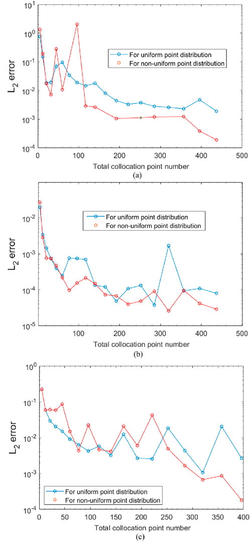
Figure 1

Figure 1. $L_2-\text{error}$ curve versus the total collocation number for example 1 (a), example 2 (b), example 3 (c).

For example 2, at time $t=1$, the variation in the total collocation point number versus the $L_2-\text{error}$ is presented in Figure 1b for both uniform and non-uniform point distributions. It can be observed that the $L_2-\text{error}$ curve converges smoothly for the non-uniform point distribution case, while there is a sharp increase for the uniform point distribution case. At the same time, the non-uniform point distribution case also performs better than the uniform case.

For example 3, at time $t=10$ with interval $\left[a,b\right]=\left[0,1\right]$, the variation in the total collocation point number versus the $L_2-\text{error}$ is presented in Figure 1c for both uniform and non-uniform point distributions. It can be observed that the $L_2-\text{error}$ curve converges smoothly for the uniform point distribution case for relatively few points. For larger points, the non-uniform case also performs better than the uniform case. Thus, we selected three different collocation numbers in the following analysis to show the numerical results. If we choose the same collocation number, the numerical results remain at the same level.

3.5 Accuracy analysis

For example 1, we fix the total collocation point number $NT=517$. In order to show the consistency between the numerical and exact solutions for different times $t=0.2$, $t=0.6$, and $t=1$, the solutions for non-uniform and uniform point distribution cases are presented in Figures 2a, b, respectively. From Figure 2a, we can observe that the numerical solutions of the non-uniform case coincide exactly with the exact solutions, while there is a relatively larger error at the two sides of the solution curve for the uniform case.

Figure 2

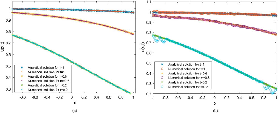
Figure 2. Numerical and analytical solutions at different times for the non-uniform case (a) and the uniform case (b).

For example 2 with fixed total collocation point number $NT=429$, Figure 3 demonstrates the strong consistency between the numerical and analytical solutions at different times $t=0.1$, $t=0.5$, and $t=1$ for the non-uniform point distribution case. It was found that the numerical solutions coincide exactly with the exact solutions for all the different times.

Figure 3

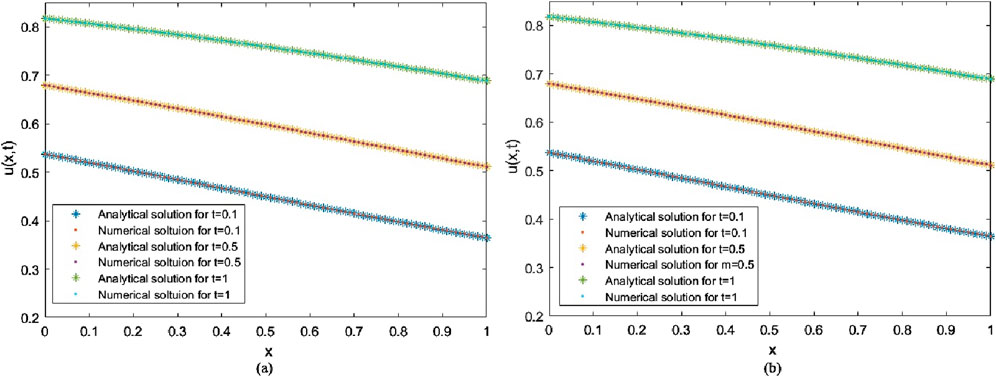
Figure 3. Numerical and analytical solutions at different times for the non-uniform case (a) and the uniform case (b).

For example 3 with interval $\left[a,b\right]=\left[-1,1\right]$ and fixed total collocation point number $NT=472$, Figure 4 illustrates the close agreement between the numerical and analytical solutions for different times $t=1$, $t=5$, and $t=10$.

Figure 4

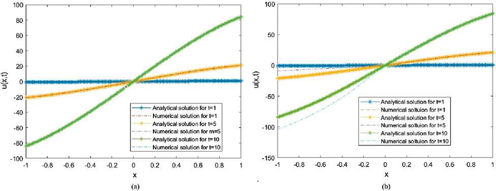
Figure 4. Numerical and analytical solutions at different times for the non-uniform case (a) and the uniform case (b).

3.6 Discussion

Numerical experiments have demonstrated the impact of two different point distributions and the total number of collocation points on solution accuracy. For all the given examples, increasing the total number of collocation points can reduce oscillations and ensure smoother convergence of the solution curve, especially for non-uniform distributions. It is notable that in cases where the total number of distribution points is relatively large, the non-uniform point distribution cases always perform better than the uniform distribution cases with higher solution accuracy. At different times, the non-uniform distribution exhibits strong consistency with the exact solution at all testing time points, while the uniform distribution shows significant errors near the domain boundaries in some cases. This may contribute to the relatively dense collocation points along the time axis; in other words, dense information at the initial boundary leads to more accurate results than in the uniform information case.

These findings emphasize the practical advantages of using non-uniform collocation with a relatively large number of points to ensure numerical stability and accuracy when solving Fisher–KPP equations.

4 Concluding remarks

In this paper, the one-level thin plate spline radial basis function collocation method is provided as an efficient and accurate approach for simulating the spatial diffusion of invasive species. The proposed method eliminates the need for complex mesh generation or adaptive re-meshing, significantly reducing the computational overhead while maintaining stability. Non-uniform point distributions yield higher accuracy than uniform distributions, especially with increased collocation point density. This work highlights the potential of mesh-free RBF-based approaches for simulating complex biological systems governed by non-linear partial differential equations.

Furthermore, the method shows promise for extension to fractional differential equations. The theoretical foundations, especially those pertaining to convergence and stability within generalized frameworks, still require significant exploration. Future research should address these directions through systematic investigation.

Data availability statement

The original contributions presented in the study are included in the article/supplementary material; further inquiries can be directed to the corresponding authors.

Author contributions

YM: Writing – review and editing, Methodology, Conceptualization, Writing – original draft, Formal Analysis, Data curation, Resources. FW: Writing – review and editing, Validation, Funding acquisition, Supervision, Formal Analysis, Resources, Writing – original draft, Software, Data curation, Visualization, Project administration, Conceptualization, Investigation, Methodology. EH: Investigation, Validation, Conceptualization, Writing – review and editing, Methodology, Writing – original draft.

Funding

The author(s) declare that financial support was received for the research and/or publication of this article. This work was partially supported by the University Natural Science Research Project of Anhui Province (Project No. 2023AH050314) and the Horizontal Scientific Research Funds in Huaibei Normal University (No. 2024340603000006).

Conflict of interest

The authors declare that the research was conducted in the absence of any commercial or financial relationships that could be construed as a potential conflict of interest.

Generative AI statement

The author(s) declare that no Generative AI was used in the creation of this manuscript.

Any alternative text (alt text) provided alongside figures in this article has been generated by Frontiers with the support of artificial intelligence and reasonable efforts have been made to ensure accuracy, including review by the authors wherever possible. If you identify any issues, please contact us.

Publisher’s note

All claims expressed in this article are solely those of the authors and do not necessarily represent those of their affiliated organizations, or those of the publisher, the editors and the reviewers. Any product that may be evaluated in this article, or claim that may be made by its manufacturer, is not guaranteed or endorsed by the publisher.

References

1. Fisher R. The wave of advance of advantageous genes. Ann Eugenics (1937) 7:355–69. doi:10.1111/j.1469-1809.1937.tb02153.x

CrossRef Full Text | Google Scholar

2. Siniukov S, Trifonov A, Shapovalov A. Examples of asymptotic solutions obtained by the complex germ method for the one-dimensional nonlocal Fisher–Kolmogorov–Petrovsky–Piskunov equation. Russ Phys J (2021) 64:1542–1552. doi:10.1007/s11182-021-02488-y

CrossRef Full Text | Google Scholar

3. Dangui-Mbani U, Sui J, Zheng L, Bin-Mohsin B, Chen G. Fisher–kolmogorov–Petrovsky–Piscounov reaction and n-Diffusion cattaneo telegraph equation. J Heat Transfer (2017) 139:074502. doi:10.1115/1.4036005

CrossRef Full Text | Google Scholar

4. Oruç Ö. An efficient wavelet collocation method for nonlinear two-space dimensional fisher–kolmogorov–petrovsky–piscounov equation and two-space dimensional extended Fisher–Kolmogorov equation. Eng Comput (2020) 36:839–56. doi:10.1007/s00366-019-00734-z

CrossRef Full Text | Google Scholar

5. Deng D, Liang Y. Analysis of a class of stabilized and structure-preserving finite difference methods for fisher-kolmogorov-petrovsky-piscounov equation. Comput Math Appl (2025) 184:86–106. doi:10.1016/j.camwa.2025.02.009

CrossRef Full Text | Google Scholar

6. Shapovalov AV, Trifonov AY. Adomian decomposition method for the one-dimensional nonlocal fisher–kolmogorov–petrovsky–piskunov equation. Russ Phys J (2019) 62:710–9. doi:10.1007/s11182-019-01768-y

CrossRef Full Text | Google Scholar

7. El-Hachem M, McCue S, Jin W, Du Y, Simpson M. Revisiting the fisher–kolmogorov–petrovsky–piskunov equation to interpret the spreading–extinction dichotomy. P Roy Soc A-math Phys (2019) 475:20190378. doi:10.1098/rspa.2019.0378

PubMed Abstract | CrossRef Full Text | Google Scholar

8. Ngamsaad W, Suantai S. Perturbative traveling-wave solution for a flux-limited reaction-diffusion morphogenesis equation. J Korean Phys Soc (2020) 76:323–9. doi:10.3938/jkps.76.323

CrossRef Full Text | Google Scholar

9. Kim S, Lee C, Lee H, Kim H, Kwak S, Hwang Y, et al. An unconditionally stable positivity-preserving scheme for the one-dimensional fisher–kolmogorov–petrovsky–piskunov equation. Discrete Dyn Nat Soc (2021). 2021:7300471–11. doi:10.1155/2021/7300471

CrossRef Full Text | Google Scholar

10. Rodrigo MR. Bounds on the critical times for the general Fisher–KPP equation. ANZIAM J (2021) 63:448–68. doi:10.1017/s1446181121000365

CrossRef Full Text | Google Scholar

11. Shapovalov AV, Kulagin AE, Siniukov SA. Pattern Formation in a nonlocal fisher–kolmogorov–petrovsky–piskunov model and in a nonlocal model of the kinetics of an metal vapor active medium. Russ Phys J (2022) 65:695–702. doi:10.1007/s11182-022-02687-1

CrossRef Full Text | Google Scholar

12. El-Hachem M, McCue S, Simpson M. Non-vanishing sharp-fronted travelling wave solutions of the Fisher–Kolmogorov model. Math Med Biol (2022) 39:226–50. doi:10.1093/imammb/dqac004

PubMed Abstract | CrossRef Full Text | Google Scholar

13. Andreu-Vilarroig C, Cortés J, Pérez C, Villanueva R. A random spatio-temporal model for the dynamics of Candida Auris in Intensive Care Units with regular cleaning. Physica A (2023) 630:129254. doi:10.1016/j.physa.2023.129254

CrossRef Full Text | Google Scholar

14. Uma D, Jafari H, Balachandar S, Venkatesh S. A mathematical modeling and numerical study for stochastic Fisher–SI model driven by space uniform white noise. Math Method Appl Sci (2023) 46:10886–902. doi:10.1002/mma.9157

CrossRef Full Text | Google Scholar

15. Kaczvinszki M, Braun S. Moving singularities of the forced Fisher–KPP equation: an asymptotic approach. SIAM J Appl Math (2024) 84:710–31. doi:10.1137/23m1552905

CrossRef Full Text | Google Scholar

16. Benito J, García A, Negreanu M, Ureña F, Vargas A. Solving nonlinear fisher–kolmogorov–petrovsky–piskunov equation using two meshless methods. Comput Part Mech (2024) 11:2373–9. doi:10.1007/s40571-024-00794-z

CrossRef Full Text | Google Scholar

17. Davydov A, Platov A, Tunitsky D. Existence of an optimal stationary solution in the KPP model under nonlocal competition. P Stekl Math (2024) 327(Suppl. 1):S66–S73. doi:10.1134/s0081543824070058

CrossRef Full Text | Google Scholar

18. Kang S, Kwak S, Hwang Y, Kim J. Positivity preserving and unconditionally stable numerical scheme for the three-dimensional modified fisher–kolmogorov–petrovsky–piskunov equation. J Comput Appl Math (2025) 457:116273. doi:10.1016/j.cam.2024.116273

CrossRef Full Text | Google Scholar

19. Zabihi F, Saffarian M. A meshless method using radial basis functions for numerical solution of the two-dimensional KdV-Burgers equation. Eur Phys J Plus (2016) 131:243. doi:10.1140/epjp/i2016-16243-y

CrossRef Full Text | Google Scholar

20. Hosseinian A, Assari P, Dehghan M. The numerical solution of nonlinear delay Volterra integral equations using the thin plate spline collocation method with error analysis. Comp Appl Math (2023) 42:83. doi:10.1007/s40314-023-02219-8

CrossRef Full Text | Google Scholar

21. Behroozi A, Vaghefi M. Global thin plate spline differential quadrature as a meshless numerical solution for two-dimensional viscous Burgers' equation. Sci Iran (2023) 30:1942–54. doi:10.24200/SCI.2022.60247.6685

CrossRef Full Text | Google Scholar

22. Zhang J, Lin J, Wang F, Gu Y. Simulation of antiplane piezoelectricity problems with multiple inclusions by the meshless method of fundamental solution with the LOOCV Algorithm for determining sources. Mathematics-Basel (2025) 13:920. doi:10.3390/math13060920

CrossRef Full Text | Google Scholar

23. Jiang Y, Wang F. A novel semi-analytical meshless method for Navier-stokes equations arising in fractured rock masses. Chin J Phys (2025) 95:1069–77. doi:10.1016/j.cjph.2025.03.007

CrossRef Full Text | Google Scholar

24. Lin Y, Wang F. A space-time meshfree method for heat transfer analysis in porous material. Phys Scripta (2024) 99:115274. doi:10.1088/1402-4896/ad8680

CrossRef Full Text | Google Scholar

25. Ju B, Qu W. Three-dimensional application of the meshless generalized finite difference method for solving the extended Fisher–Kolmogorov equation. Appl Math Lett (2023) 136:108458. doi:10.1016/j.aml.2022.108458

CrossRef Full Text | Google Scholar

26. Zhang J, Wang F, Hou E. The conical radial basis function for partial differential equations. J Math (2020) 2020:6664071–7. doi:10.1155/2020/6664071

CrossRef Full Text | Google Scholar