Coupling microscopic and mesoscopic models for crowd dynamics with emotional contagion

We are interested in modeling and simulating the dynamics of human crowds, where the spreading of an emotion (specifically fear) influences the pedestrians’ behavior. Our focus is on crowd dynamics in venues where dense aggregations might occur within a rarefied crowd (e.g., an airport terminal) and emotional states evolve in space and time as the result of a threat (e.g., a gunshot). In the parts of the venue where crowd density is low, we consider a microscopic, individual-based model inspired by Newtonian mechanics. In this model, the fear level of each pedestrian influences their walking speed and is affected by the fear levels of the people in their vicinity. The mesoscopic model is derived from the microscopic model via a mean-field limit approach. This ensures that the two types of models are based on the same principles and analogous parameters. The mesoscopic model is adopted in the parts of the venue where crowd density is higher, i.e., we use the crowd density as a regime indicator. We propose interface conditions to be imposed at the boundary between the regions of the domain where microscopic and mesoscopic models are used. We note that we do not consider dangerously high-density crowd scenarios, for which a macroscopic (continuum) model would be more appropriate. We test our microscopic-to-mesoscopic model on problems involving a crowd walking through a corridor or evacuating from a square.

1 Introduction

Crowds have the ability to act, think, and adapt their own movement strategies in response to environmental cues. This feature, possessed by living systems in general, sets them apart from inert matter, which follows deterministic laws of physics and behaves predictably under given conditions. It also makes the mathematical modeling of crowd dynamics particularly challenging. In fact, to be accurate even in situations when people alter their typical walking strategy in response to an external cue (e.g., a gunshot or a propagating fire), a model of crowd dynamics needs to go beyond the principles of classical mechanics. Specifically, it needs to incorporate mechanisms to account for heterogeneous behavior of individual entities and their interactions, together with the effect of an emotional state (e.g., fear) on both individuals and interactions. See, e.g., [1–7]. Such a model could be instrumental in improving crowd management in venues like airport terminals or concert arenas.

Microscopic, such as agent-based models, effectively capture individual variability since they allow each agent to adopt a unique walking strategy. See, e.g., [8–12]. For a comprehensive overview of agent-based models that implement emotional contagion in crowd simulations, we refer the reader to [13]. Unfortunately, microscopic models struggle with scalability. Specifically, they cannot accurately represent complex, non-local, and nonlinearly additive interactions as crowd size increases. Mesoscopic or kinetic models (see, e.g. [5–7, 14–18]) offer an alternative that can reproduce complex interactions in crowds. Inspired by the kinetic theory of gases, these models consider individuals as active particles, instead of passive particles, i.e., particles that interact in a conservative and reversible manner as in traditional gas dynamics. The consequence is that interactions in kinetic models for crowd dynamics are irreversible, non-conservative and, in some cases, nonlocal and nonlinearly additive [6, 7, 15]. Therefore, kinetic models offer a powerful tool to overcome the limitations of agent-based models in capturing complex interactions. However, these models, which are Boltzmann-type evolution equations for the statistical distribution of pedestrian positions and velocities, become computationally expensive when the size of the computational domain is large.

This paper proposes a hybrid approach to the study of crowds under the influence of a spreading emotion aiming to combine the advantages of microscopic and kinetic models, while lessening the respective limitations. The starting point for our hybrid model is a microscopic model from [19] in which the emotional state (i.e., the fear level) of each person influences their walking speed and is affected by the emotional state of the people in their vicinity. Note that the emotional state is introduced as a variable that, in response to interactions with other people, can change in space and time and, in turn, alter the walking strategy, as it happens in real-life situations [4]. Through a mean-field limit approach, from the microscopic model we derived a (Bhatnagar–Gross–Krook-like) kinetic model. This operation in 1D is presented in [19], while here we extend it to 2D and propose how the kinetic and microscopic models can be interfaced, so that each model can be used where its use is most appropriate. Specifically, the microscopic model is adopted in the parts of the domain where the crowd density is lower than a prescribed value since in this case such model is computationally cheap and accurate. Where the density is above the prescribed value and the microscopic model loses accuracy and computational efficiency, we adopt the kinetic model. Since we limit the size of the domain where the kinetic model holds, our hybrid microscopic-to-mesoscopic approach remains computationally efficient. Figure 1 shows a picture of a real crowd with mixed density: the vertical black line separates the higher density crowd (left), which would be simulated with the kinetic model, from the lower density crowd (right), which would be simulated with the microscopic model.

Figure 1

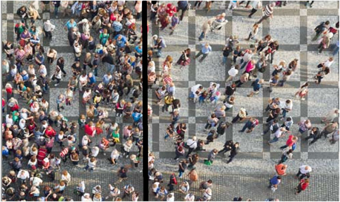
Figure 1. Example of a mixed density crowd, with dense aggregations (left of the black line) near low-density regions (right of the black line).

In addition to the advantages discussed so far, our hybrid model stems from a multiscale vision, i.e., the dynamics at the microscopic scale define the conceptual basis toward the derivation of the models at a higher scale (mesoscopic). The reader interested in the further derivation of a macroscopic model from the kinetic model is referred to [19], where results are limited to one space dimension. At the macroscopic level, the crowd is seen as a continuum and thus macroscopic models are suited for densely packed crowds. It is shown in [19] that the kinetic description provides better resolution than the macroscopic model whose viscosity solution becomes incorrect when the characteristics at the particle level cross. Because of this, we do not consider the macroscopic model and how it interfaces to the models at the lower scales.

Following [19], for simplicity we assume that the walking direction is prescribed. This means that our model cannot reproduce the tendency of an individual in a stressful situation to follow the stream of people, also referred to as herding in the literature [20]. The reader interested in kinetic models that allow for a change in walking direction as a results of interactions with other people and the environment (i.e., walls and other kinds of obstacle) is referred to [16–18, 21–25]. We remark that only in [23] the emotional state is treated as a variable, while it is parameterized as a constant in space and time in [16, 18, 21, 22, 25] and as a function of space and time in [17, 24].

We assess our hybrid method through test cases in one and two dimensions. The tests in 1D represent one-directional motion through a corridor, where half of the people have a high fear level and the remaining half have no fear at all. This situation leads to a localized high crowd density as the panicked people walk faster than the non-panicked. The 2D tests also create a localized high-density region, resulting from a scenario similar to a group of panicked people trying to evacuate a square.

The rest of the paper is organized as follows. Section 2 briefly recalls the derivation of the 1D mesoscopic model from the 1D microscopic model from [19], extends the derivation to 2D and then presents the discretization of the 2D microscopic and mesoscopic models. The interface conditions that allow to use microscopic and mesoscopic models in different parts of a given domain are discussed in Section 3. Section 4 presents the numerical results and conclusions are drawn in Section 5.

2 From microscopic to mesoscopic

2.1 In one dimension

We consider a system of $N$ agents that are described by their positions $x_i(t),i=1,\dots ,N$ in spatial domain $\mathrm{\Omega }\subset \mathbb{R}$ and fear levels $q_i(t),i=1,\dots ,N$ for time $t$ belonging to a time interval of interest $(0,T]$. Each agent moves with speed equal to the agent’s fear level and the fear level of an agent tends to the local average of fear levels of nearby agents. The microscopic model, also called agent-based, is described by the following system of ordinary differential equations:

$\frac{d{x}_i}{dt}=q_i,\frac{d{q}_i}{dt}=\gamma \left(q_i^{*}-q_i\right),(1)$

for $i=1,\dots ,N$, where $q_i^{*}$, the average fear level for agent $i$, defined as:

$q_i^{*}=\frac{{\sum }_{j=1}^N{\kappa }_{i,j}{q}_j}{{\sum }_{j=1}^N{\kappa }_{i,j}},(2)$

${\kappa }_{i,j}=\kappa (|x_i-x_j|)$ being an interaction kernel. One of the commonly used formulas for this kernel is

$\kappa \left(r\right)=\frac{R}{\left(r^2+R^2\right)\pi },r\ge 0,(3)$

see for example, [19]. Parameter $R>0$ in Equation 3 characterizes the radius of interactions. Parameter $\gamma$ in Equation 1 describes the interaction strength. For simplicity, we assume that the interaction strengths of all agents are equal, although for one test in Section 4.1 we will make its value variable from one agent to the other.

We note that Equation 1 is simply Newton’s law, assuming that fear is the only driver for motion. In this simple model, every agent has the same mass, which then gets normalized to 1.

The kinetic formulation is derived from Equations 1, 2 via a mean-field limit approach. For this, we denote the empirical distribution density as:

$f^N\left(x,q,t\right)=\frac{1}{N}{\displaystyle \sum _{i=1}^N}\delta \left(x-x_i\left(t\right)\right)\delta \left(q-q_i\left(t\right)\right),(4)$

where $(x_i(t),q_i(t))$ is as in Equation 1, and $\delta$ represents the Dirac delta function. To obtain the kinetic model, let $\psi \in C_0^1({\mathbb{R}}^2)$ be a test function, multiply Equation 4 by $\psi$, integrate with respect to space and fear level over the respective domain and differentiate in time:

$\begin{array}{ll}\hfill \frac{d}{dt}\iint f^N\left(x,q,t\right)\psi \left(x,q\right)dxdq& =\frac{1}{N}{\displaystyle \sum _{i=1}^N}\frac{d}{dt}\iint \delta \left(x-x_i\left(t\right)\right)\hfill \\ \hfill & \delta \left(q-q_i\left(t\right)\right)\psi \left(x,q\right)dxdq.\hfill \end{array}$

By manipulating the above equation as explained in [19], one gets the following integral equation:

$\begin{array}{ll}\hfill \iint \psi & \left[f^N{\left(x,q,t\right)}_t+{\left(f^N\left(x,q,t\right)\cdot q\right)}_x\right.\hfill \\ \hfill & \left.+\gamma {\left(\left[\frac{\left(\kappa \ast m_{f^N}\right)\left(x,t\right)}{\left(\kappa \ast {\rho }_{f^N}\right)\left(x,t\right)}-q\right]f^N\left(x,q,t\right)\right)}_q\right]dxdq=0,\hfill \end{array}(5)$

where

$\begin{array}{ll}\hfill m_{f^N}\left(x,t\right)& =\frac{1}{N}{\displaystyle \sum _{j=1}^N}\delta \left(x-x_j\right)q_j=\iint \frac{1}{N}{\displaystyle \sum _{j=1}^N}\delta \left(x-x_j\right)\delta \left(q-q_j\right)qdxdq\hfill \\ \hfill & =\int f^N\left(x,q,t\right)qdq,\hfill \end{array}$

and

${\rho }_{f^N}\left(x,t\right)=\frac{1}{N}{\displaystyle \sum _{i=1}^N}\delta \left(x-x_i\right)=\int f^N\left(x,q,t\right)dq.$

Since $\psi$ is an arbitrary test function, Equation 5 leads to the following equation:

$f_t^N+{\left(f^{N}q\right)}_x+\gamma {\left(\left[\frac{\left(\kappa \ast m_{f^N}\right)\left(x,t\right)}{\left(\kappa \ast {\rho }_{f^N}\right)\left(x,t\right)}-q\right]f^N\right)}_q=0,$

which can be rewritten as:

$f_t^N+{\left(q{f}^N\right)}_x+\gamma {\left(\left(q^{*}-q\right)f^N\right)}_q=0,$

where the local average fear level $q^{*}(t,x)$ is given by:

$q^{*}\left(x,t\right)=\frac{\iint \kappa \left(|x-y|\right)f^N\left(y,q,t\right)qdqdy}{\iint \kappa \left(|x-y|\right)f^N\left(y,q,t\right)dqdy}.$

Under appropriate compactness assumptions, the empirical distribution $f^N$ converges weakly to a limiting distribution $f(x,q,t)$ as $N\to \infty$, resulting in the following kinetic equation:

$f_t+{\left(qf\right)}_x+\gamma {\left(\left(q^{*}-q\right)f\right)}_q=0.$

2.2 In two dimensions

The $N$ agents are now described by their positions ${\mathbf{x}}_i(t)=(x_i(t),y_i(t))$ within domain $\mathrm{\Omega }\subset {\mathbb{R}}^2$ and fear levels $q_i(t),i=1,\dots ,N$. The time interval of interest is $(0,T]$. Each agent moves with speed equal to their fear level and with a prescribed direction ${\theta }_i$. This could be, e.g., the direction to the nearest exit if we are considering an evacuation scenario. So, we obtain the following microscopic model:

$\frac{d{\mathbf{x}}_i}{dt}=q_i\left(\cos {\theta }_i,\sin {\theta }_i\right),\frac{d{q}_i}{dt}=\gamma \left(q_i^{*}-q_i\right),(6)$

for $i=1,\dots ,N$, where $q_i^{*}$, the average fear level for agent $i$, defined as:

$q_i^{*}=\frac{{\sum }_{j=1}^N{\kappa }_{i,j}{q}_j}{{\sum }_{j=1}^N{\kappa }_{i,j}},$

${\kappa }_{i,j}=\kappa (|{\mathbf{x}}_i-{\mathbf{x}}_j)|$ being an interaction kernel. We consider again the kernel in Equation 3.

For the derivation of the kinetic model, we follow the same steps used in 1D. We denote the empirical distribution density as:

$f^N\left(\mathbf{x},q,t\right)=\frac{1}{N}{\displaystyle \sum _{i=1}^N}\delta \left(\mathbf{x}-{\mathbf{x}}_i\left(t\right)\right)\delta \left(q-q_i\left(t\right)\right),(7)$

where $({\mathbf{x}}_i(t),q_i(t))$ is as in Equation 6 and $\delta$ is the Dirac delta function. We multiply Equation 7 by a test function $\psi \in C_0^1({\mathbb{R}}^3)$, integrate with respect to space and fear level and differentiate in time:

$\begin{array}{ll}\hfill \frac{d}{dt}\iint f^N\left(\mathbf{x},q,t\right)\psi \left(\mathbf{x},q\right)d\mathbf{x}dq& =\frac{1}{N}{\displaystyle \sum _{i=1}^N}\frac{d}{dt}\iint \delta \left(\mathbf{x}-{\mathbf{x}}_i\left(t\right)\right)\delta \hfill \\ \hfill & \left(q-q_i\left(t\right)\right)\psi \left(\mathbf{x},q\right)d\mathbf{x}dq.\hfill \end{array}$

Since $\iint \delta (\mathbf{x}-{\mathbf{x}}_i(t))\delta (q-q_i(t))\psi (\mathbf{x},q)d\mathbf{x}dq=\psi ({\mathbf{x}}_i(t),q_i(t))$, then

$\begin{array}{ll}\hfill \frac{d}{dt}\iint f^N\left(\mathbf{x},q,t\right)\psi \left(\mathbf{x},q\right)d\mathbf{x}dq& =\frac{1}{N}{\displaystyle \sum _{i=1}^N}\frac{d}{dt}\psi \left({\mathbf{x}}_i\left(t\right),q_i\left(t\right)\right)\hfill \\ \hfill & =\frac{1}{N}{\displaystyle \sum _{i=1}^N}\left(\left({\psi }_x\left({\mathbf{x}}_i,q_i\right),{\psi }_y\left({\mathbf{x}}_i,q_i\right)\right)\cdot \right.\hfill \\ \hfill & \left.\frac{d{\mathbf{x}}_i}{dt},+,{\psi }_q,\left({\mathbf{x}}_i,q_i\right),\frac{d{q}_i}{dt}\right).\hfill \end{array}$

By plugging Equation 6 into the above equation, we obtain:

$\begin{array}{ll}\hfill & \frac{d}{dt}\iint f^N\left(\mathbf{x},q,t\right)\psi \left(\mathbf{x},q\right)d\mathbf{x}dq\hfill \\ \hfill & =\frac{1}{N}{\displaystyle \sum _{i=1}^N}\left(\left({\psi }_x\left({\mathbf{x}}_i,q_i\right),{\psi }_y\left({\mathbf{x}}_i,q_i\right)\right)\cdot q_i\left(\cos {\theta }_i,\sin {\theta }_i\right)+{\psi }_q\left({\mathbf{x}}_i,q_i\right)\gamma \left(q_i^{*}-q_i\right)\right)\hfill \\ \hfill & =\frac{1}{N}{\displaystyle \sum _{i=1}^N}\iint \delta \left(\mathbf{x}-{\mathbf{x}}_i\right)\delta \left(q-q_i\right)\left({\psi }_x\left(\mathbf{x},q\right)\cos \theta +{\psi }_y\left(\mathbf{x},q\right)\sin \theta \right)qd\mathbf{x}dq\hfill \\ \hfill & +\frac{\gamma }{N}{\displaystyle \sum _{i=1}^N}{\psi }_q\left({\mathbf{x}}_i,q_i\right)\left(\frac{{\sum }_{j=1}^N{\kappa }_{i,j}{q}_j}{{\sum }_{j=1}^N{\kappa }_{i,j}}-q_i\right).\hfill \end{array}$

Using Equation 7, we get

$\begin{array}{ll}\hfill \frac{d}{dt}\iint f^N\left(\mathbf{x},q,t\right)\psi \left(\mathbf{x},q\right)d\mathbf{x}dq& =\iint f^N\left(\mathbf{x},q,t\right)\left({\psi }_x\left(\mathbf{x},q\right)\cos \theta +{\psi }_y\left(\mathbf{x},q\right)\sin \theta \right)\hfill \\ \hfill & qd\mathbf{x}dq+\frac{\gamma }{N}{\displaystyle \sum _{i=1}^N}{\psi }_q\left({\mathbf{x}}_i,q_i\right)\left(\frac{{\sum }_{j=1}^N{\kappa }_{i,j}{q}_j}{{\sum }_{j=1}^N{\kappa }_{i,j}}-q_i\right).\hfill \end{array}(8)$

We have:

$\begin{array}{ll}\hfill \frac{1}{N}{\displaystyle \sum _{j=1}^N}{\kappa }_{i,j}{q}_j& =\frac{1}{N}{\displaystyle \sum _{j=1}^N}\kappa \left(|{\mathbf{x}}_i-{\mathbf{x}}_j|\right)q_j=\int \kappa \left(|{\mathbf{x}}_i-\mathbf{x}|\right)\frac{1}{N}{\displaystyle \sum _{j=1}^N}\delta \left(\mathbf{x}-{\mathbf{x}}_j\right)\hfill \\ \hfill & q_{j}d\mathbf{x}=\iint \kappa \left(|{\mathbf{x}}_i-\mathbf{x}|\right)m_{f^N}\left(\mathbf{x},t\right)d\mathbf{x}=\left(\kappa \ast m_{f^N}\right)\left({\mathbf{x}}_i,t\right),\hfill \end{array}(9)$

where

$\begin{array}{ll}\hfill m_{f^N}\left(x,y,t\right)& =\frac{1}{N}{\displaystyle \sum _{j=1}^N}\delta \left(\mathbf{x}-{\mathbf{x}}_j\right)q_j=\iint \frac{1}{N}{\displaystyle \sum _{j=1}^N}\delta \left(\mathbf{x}-{\mathbf{x}}_j\right)\delta \left(q-q_j\right)\hfill \\ \hfill & qd\mathbf{x}dq=\int f^N\left(\mathbf{x},q,t\right)qdq.\hfill \end{array}$

Similarly, we have:

$\begin{array}{ll}\hfill \frac{1}{N}{\displaystyle \sum _{j=1}^N}{\kappa }_{ij}& =\int \kappa \left(|{\mathbf{x}}_i-\mathbf{x}|\right)\left(\frac{1}{N}{\displaystyle \sum _{j=1}^N}\delta \left(\mathbf{x}-{\mathbf{x}}_j\right)\right)d\mathbf{x}\hfill \\ \hfill & =\int \kappa \left(|{\mathbf{x}}_i-\mathbf{x}|\right){\rho }_{f^N}\left(\mathbf{x},t\right)d\mathbf{x}=\left(\kappa \ast {\rho }_{f^N}\right)\left({\mathbf{x}}_i,t\right),\hfill \end{array}(10)$

where

${\rho }_{f^N}\left(\mathbf{x},t\right)=\frac{1}{N}{\displaystyle \sum _{i=1}^N}\delta \left(\mathbf{x}-{\mathbf{x}}_i\right)=\int f^N\left(\mathbf{x},q,t\right)dq.$

Using Equations 9, 10, the second term at the right-hand side of Equation 8 can be written as:

$\begin{array}{ll}\hfill & \frac{\gamma }{N}{\displaystyle \sum _{i=1}^N}{\psi }_q\left({\mathbf{x}}_i,q_i\right)\left[\frac{\left(\kappa \ast m_{f^N}\right)\left({\mathbf{x}}_i,t\right)}{\left(\kappa \ast {\rho }_{f^N}\right)\left({\mathbf{x}}_i,t\right)}-q_i\right]\hfill \\ \hfill & =\gamma \iint {\psi }_q\left(\mathbf{x},q\right)\left[\frac{\left(\kappa \ast m_{f^N}\right)\left(\mathbf{x},t\right)}{\left(\kappa \ast {\rho }_{f^N}\right)\left(\mathbf{x},t\right)}-q\right]\frac{1}{N}{\displaystyle \sum _{i=1}^N}\delta \left(\mathbf{x}-{\mathbf{x}}_i\right)\delta \left(q-q_i\right)d\mathbf{x}dq\hfill \\ \hfill & =\gamma \iint {\psi }_q\left(\mathbf{x},q\right)\left[\frac{\left(\kappa \ast m_{f^N}\right)\left(\mathbf{x},t\right)}{\left(\kappa \ast {\rho }_{f^N}\right)\left(\mathbf{x},t\right)}-q\right]f^N\left(\mathbf{x},q,t\right)d\mathbf{x}dq.\hfill \end{array}$

Thus, Equation 8 becomes

$\begin{array}{ll}\hfill \frac{d}{dt}\iint f^N\left(\mathbf{x},q,t\right)\psi \left(\mathbf{x},q\right)d\mathbf{x}dq& =\iint f^N\left(\mathbf{x},q,t\right)\left({\psi }_x\left(\mathbf{x},q\right)\cos \theta +{\psi }_y\left(\mathbf{x},q\right)\sin \theta \right)\hfill \\ \hfill & qd\mathbf{x}dq+\gamma \iint {\psi }_q\left(\mathbf{x},q\right)\left[\frac{\left(\kappa \ast m_{f^N}\right)\left(\mathbf{x},t\right)}{\left(\kappa \ast {\rho }_{f^N}\right)\left(\mathbf{x},t\right)}-q\right]\hfill \\ \hfill & f^N\left(\mathbf{x},q,t\right)d\mathbf{x}dq\hfill \end{array}$

Integrating the terms on the right-hand side of this equation by parts, assuming that $\psi$ vanishes at the boundaries, and rearranging the terms, we get:

$\begin{array}{ll}\hfill \iint \psi & \left[f^N{\left(\mathbf{x},q,t\right)}_t+{\left(q\cos \theta f^N\left(\mathbf{x},q,t\right)\right)}_x+{\left(q\sin \theta f^N\left(\mathbf{x},q,t\right)\right)}_y\right.\hfill \\ \hfill & \left.+\gamma {\left(\left[\frac{\left(\kappa \ast m_{f^N}\right)\left(\mathbf{x},t\right)}{\left(\kappa \ast {\rho }_{f^N}\right)\left(\mathbf{x},t\right)}-q\right]f^N\left(\mathbf{x},q,t\right)\right)}_q\right]d\mathbf{x}dq=0.\hfill \end{array}$

Since $\psi$ is an arbitrary test function, this leads to:

$f_t^N+{\left(q\cos \theta f^N\right)}_x+{\left(q\sin \theta f^N\right)}_y+\gamma {\left(\left[\frac{\left(\kappa \ast m_{f^N}\right)}{\left(\kappa \ast {\rho }_{f^N}\right)}-q\right]f^N\right)}_q=0,$

which can be rewritten as:

$f_t^N+{\left(q\cos \theta f^N\right)}_x+{\left(q\sin \theta f^N\right)}_y+\gamma {\left(\left(q^{*}-q\right)f^N\right)}_q=0,$

where the local average fear level $q^{*}$ is given by:

$q^{*}\left(\mathbf{x},t\right)=\frac{\iint \kappa \left(|\mathbf{x}-{\mathbf{x}}^{\prime }|\right)f^N\left({\mathbf{x}}^{\prime },q,t\right)qd{\mathbf{x}}^{\prime }dq}{\iint \kappa \left(|\mathbf{x}-{\mathbf{x}}^{\prime }|\right)f^N\left({\mathbf{x}}^{\prime },q,t\right)d{\mathbf{x}}^{\prime }dq}.$

Under appropriate compactness assumptions, the empirical distribution $f^N$ converges weakly to a limiting distribution $f(\mathbf{x},q,t)$ as $N\to \infty$, resulting in the following kinetic equation:

$f_t+{\left(q\cos \theta f\right)}_x+{\left(q\sin \theta f\right)}_y+\gamma {\left(\left(q^{*}-q\right)f\right)}_q=0.(11)$

2.3 Discretization of the 2D models

We use the explicit Euler scheme for the system of ordinary differential Equation 8. Let $\mathrm{\Delta }t$ be a time step and $t_n=n\mathrm{\Delta }t$, $n=0,\dots ,\frac{T}{\mathrm{\Delta }t}$. Denote by $({\mathbf{x}}_i^n,q_i^n)$ the values of the position and the fear level of agent $i$ at time $t_n$. The values at time $t_{n+1}$ are given by

${\mathbf{x}}_i^{n+1}={\mathbf{x}}_i^n+q_i^n\left(\cos {\theta }_i^n,\sin {\theta }_i^n\right)\mathrm{\Delta }t,q_i^{n+1}=q_i^n+\gamma \left(q_i^{*,n}-q_i^n\right)\mathrm{\Delta }t,(12)$

with

$q_i^{*,n}=\frac{{\sum }_{j=1}^N\kappa \left(|{\mathbf{x}}_i^n-{\mathbf{x}}_j^n|\right)q_j^n}{{\sum }_{j=1}^N\kappa \left(|{\mathbf{x}}_i^n-{\mathbf{x}}_j^n|\right)}.$

Next, we consider the discretization of Equation 11 in space, time, and fear level using a finite difference method. We assume that $\mathbf{x}\in \mathrm{\Omega }=[-D,D]\times [-D,D]$, for given $D$. We partition $\mathrm{\Omega }$ using mesh size $\mathrm{\Delta }x$ along the $x$ axis and $\mathrm{\Delta }y$ along the $y$ axis, so to obtain cells:

${\mathrm{\Omega }}_{i,j}=\left(x_{i-\frac{1}{2}},x_{i+\frac{1}{2}}\right)\times \left(y_{j-\frac{1}{2}},y_{j+\frac{1}{2}}\right),x_{i+\frac{1}{2}}=x_i+\frac{\mathrm{\Delta }x}{2},y_{j+\frac{1}{2}}=y_j+\frac{\mathrm{\Delta }y}{2},$

where the centers of the cells $(x_i,y_j)$ are given by $(i\mathrm{\Delta }x-D,j\mathrm{\Delta }y-D)$, for $i=\mathrm{0,1},\dots ,N_x$ and $j=\mathrm{0,1},\dots ,N_y$, where $N_x=2D/\mathrm{\Delta }x$, and $N_y=2D/\mathrm{\Delta }y$. The fear level varies in interval $[\mathrm{0,1}]$, with $q=0$ indicating no stress and $q=1$ indicating the highest stress level. Interval [0,1] is partitioned into intervals of equal length $\mathrm{\Delta }q$:

$\left(q_{j-\frac{1}{2}},q_{j+\frac{1}{2}}\right),q_{j+\frac{1}{2}}=q_j+\frac{\mathrm{\Delta }q}{2},$

where the centers of the cells $q_j$ are given by $q_j=j\mathrm{\Delta }q$, for $j=\mathrm{0,1},\dots ,N_q$, with $N_q=1/\mathrm{\Delta }q$. These partitions of $\mathrm{\Omega }$ and [0,1] induce a partition of the 3D domain $\mathrm{\Omega }\times [\mathrm{0,1}]$ into 3D cells.

Let $(0,T]$ be the time interval of interest and set the time step $\mathrm{\Delta }t$ to

$\mathrm{\Delta }t=\frac{1}{2}\min \left\{\frac{\mathrm{\Delta }x}{{\max }_j{q}_j},\frac{\mathrm{\Delta }y}{{\max }_j{q}_j},\frac{\mathrm{\Delta }q}{2\gamma {\max }_j{q}_j}\right\}.(13)$

to satisfy the Courant–Friedrichs–Lewy (CFL) condition (see, e.g. [26]). Further, we denote $t^n=n\mathrm{\Delta }t$, $n=\mathrm{0,1},\dots ,T/\mathrm{\Delta }t$, and for any given quantity $g$, its approximation at a specific time point $t^n$ is denoted with $g^n$.

The finite difference method produces an approximation of the average over the cell

$f_{j,k,l}^n\approx \frac{1}{|{\mathrm{\Omega }}_{j,k}|\mathrm{\Delta }q}{\int }_{{\mathrm{\Omega }}_{j,k}}{\int }_{q_{l-\frac{1}{2}}}^{q_{l+\frac{1}{2}}}f\left(\mathbf{x},q,t^n\right)d\mathbf{x}dq.$

To write the finite difference discretization of Equation 11, we introduce

$\begin{array}{ll}\hfill q_{j,k}^{*,n}& =\frac{{\sum }_l{\sum }_{\bar{j}}{\sum }_{\bar{k}}{\kappa }_{j,\bar{j},k,\bar{k}}{f}_{\bar{j},\bar{k},l}^n{q}_l\mathrm{\Delta }q|{\mathrm{\Omega }}_{\bar{j},\bar{k}}|}{{\sum }_l{\sum }_{\bar{j}}{\sum }_{\bar{k}}{\kappa }_{j,\bar{j},k,\bar{k}}{f}_{\bar{j},\bar{k},l}^n\mathrm{\Delta }q|{\mathrm{\Omega }}_{\bar{j},\bar{k}}|},\hfill \\ \hfill & {\kappa }_{j,\bar{j},k,\bar{k}}=\frac{R}{\left({\left(x_j-x_{\bar{j}}\right)}^2+{\left(y_k-y_{\bar{k}}\right)}^2+R^2\right)\pi }.\hfill \end{array}(14)$

Additionally, let $\varphi$ be slope limiter function. For the numerical results in Section 4, we will consider and compare two slope limiters: the van Leer limiter

$\varphi \left(\theta \right)=\frac{|\theta |+\theta }{1+|\theta |},$

and the minmod slope limiter

$\varphi \left(\theta \right)=\left\{\begin{array}{cc}\mathrm{0\hspace{0.17em}\hspace{0.17em}}\hfill & \text{\hspace{1em}if\hspace{1em}}\theta \le 0,\hfill \\ \mathrm{\theta \hspace{0.17em}\hspace{0.17em}}\hfill & \text{\hspace{1em}if\hspace{1em}}0\le \theta \le 1,\hfill \\ \mathrm{1\hspace{0.17em}\hspace{0.17em}}\hfill & \text{\hspace{1em}if\hspace{1em}}\theta \ge 1.\hfill \end{array}\right.$

See, e.g., [26] for more details.

A finite difference scheme for Equation 11 is as follows: At time step $t^{n+1}$, find $f_{j,k,l}^{n+1}$ for $j=1,\dots ,N_x-1$, $k=1,\dots ,N_x-1$ and $l=1,\dots ,N_q-1$, such that:

$\begin{array}{ll}\hfill \frac{f_{j,k,l}^{n+1}-f_{j,k,l}^n}{\mathrm{\Delta }t}& +\frac{{\eta }_{j+\frac{1}{2},k,l}^n-{\eta }_{j-\frac{1}{2},k,l}^n}{\mathrm{\Delta }x}+\frac{{\zeta }_{j,k+\frac{1}{2},l}^n-{\zeta }_{j,k-\frac{1}{2},l}^n}{\mathrm{\Delta }y}+\gamma \frac{{\xi }_{j,k,l+\frac{1}{2}}^n-{\xi }_{j,k,l-\frac{1}{2}}^n}{\mathrm{\Delta }q}\hfill \\ \hfill & +\gamma \frac{C_{j,k,l+\frac{1}{2}}^n-C_{j,k,l-\frac{1}{2}}^n}{\mathrm{\Delta }q}=0,\hfill \end{array}$

where the flux in $x$ variable is

${\eta }_{j+\frac{1}{2},k,l}^n={\eta }_{j+\frac{1}{2},k,l}^{n,+}+{\eta }_{j+\frac{1}{2},k,l}^{n,-},$

with

$\begin{array}{ll}\hfill {\eta }_{j+\frac{1}{2},k,l}^{n,+}& ={\eta }_{j,k,l}^{n,+}+\frac{\mathrm{\Delta }x}{2}{\sigma }_{j,k,l}^{n,+},{\eta }_{j+\frac{1}{2},k,l}^{n,-}={\eta }_{j+1,k,l}^{n,-}-\frac{\mathrm{\Delta }x}{2}{\sigma }_{j+1,k,l}^{n,-},\hfill \\ \hfill & {\eta }_{j,k,l}^{n,+}=\frac{|q_l\cos {\theta }_{j,k}|+q_l\cos {\theta }_{j,k}}{2}{f}_{j,k,l}^n,\hfill \\ \hfill & {\eta }_{j,k,l}^{n,-}=\frac{q_l\cos {\theta }_{j,k}-|q_l\cos {\theta }_{j,k}|}{2}{f}_{j,k,l}^n,\hfill \\ \hfill & {\sigma }_{j,k,l}^{n,+}=\frac{{\eta }_{j+1,k,l}^{n,+}-{\eta }_{j,k,l}^{n,+}}{\mathrm{\Delta }x}\varphi \left(\frac{{\eta }_{j,k,l}^{n,+}-{\eta }_{j-1,k,l}^{n,+}}{{\eta }_{j+1,k,l}^{n,+}-{\eta }_{j,k,l}^{n,+}}\right),\hfill \\ \hfill & {\sigma }_{j,k,l}^{n,-}=\frac{{\eta }_{j,k,l}^{n,-}-{\eta }_{j-1,k,l}^{n,-}}{\mathrm{\Delta }x}\varphi \left(\frac{{\eta }_{j+1,k,l}^{n,-}-{\eta }_{j,k,l}^{n,-}}{{\eta }_{j,k,l}^{n,-}-{\eta }_{j-1,k,l}^{n,}}\right),\hfill \end{array}$

and the flux in $y$ variable is

${\zeta }_{j,k+\frac{1}{2},l}^n={\zeta }_{j,k+\frac{1}{2},l}^{n,+}+{\zeta }_{j,k+\frac{1}{2},l}^{n,-},$

with

$\begin{array}{ll}\hfill {\zeta }_{j,k+\frac{1}{2},l}^{n,+}& ={\zeta }_{j,k,l}^{n,+}+\frac{\mathrm{\Delta }x}{2}{\omega }_{j,k,l}^{n,+},{\zeta }_{j+\frac{1}{2},k,l}^{n,-}={\zeta }_{j,k+1,l}^{n,-}-\frac{\mathrm{\Delta }x}{2}{\omega }_{j,k+1,l}^{n,-},\hfill \\ \hfill & {\zeta }_{j,k,l}^{n,+}=\frac{|q_l\sin {\theta }_{j,k}|+q_l\sin {\theta }_{j,k}}{2}{f}_{j,k,l}^n,\hfill \\ \hfill & {\zeta }_{j,k,l}^{n,-}=\frac{q_l\sin {\theta }_{j,k}-|q_l\sin {\theta }_{j,k}|}{2}{f}_{j,k,l}^n,\hfill \\ \hfill & {\omega }_{j,k,l}^{n,+}=\frac{{\zeta }_{j,k+1,l}^{n,+}-{\zeta }_{j,k,l}^{n,+}}{\mathrm{\Delta }y}\varphi \left(\frac{{\zeta }_{j,k,l}^{n,+}-{\zeta }_{j,k-1,l}^{n,+}}{{\zeta }_{j,k+1,l}^{n,+}-{\zeta }_{j,k,l}^{n,+}}\right),\hfill \\ \hfill & {\omega }_{j,k,l}^{n,-}=\frac{{\zeta }_{j,k,l}^{n,-}-{\zeta }_{j,k-1,l}^{n,-}}{\mathrm{\Delta }y}\varphi \left(\frac{{\zeta }_{j,k+1,l}^{n,-}-{\zeta }_{j,k,l}^{n,-}}{{\zeta }_{j,k,l}^{n,-}-{\zeta }_{j,k-1,l}^{n,}}\right).\hfill \end{array}$

The flux and flux limiter in $q$ is

$\begin{array}{ll}\hfill {\xi }_{j,k,l+\frac{1}{2}}^n& =\frac{|q_{j,k}^{*,n}-q_{l+\frac{1}{2}}^n|+\left(q_{j,k}^{*,n}-q_{l+\frac{1}{2}}^n\right)}{2}{f}_{j,k,l}^n\hfill \\ \hfill & +\frac{|q_{j,k}^{*,n}-q_{l+\frac{1}{2}}^n|-\left(q_{j,k}^{*,n}-q_{l+\frac{1}{2}}^n\right)}{2}{f}_{j,k,l+1}^n,\hfill \\ \hfill & C_{j,k,l+\frac{1}{2}}^n=\frac{1}{2}|s_{j,k,l+\frac{1}{2}}^n|\left(1-\frac{\mathrm{\Delta }t}{\mathrm{\Delta }q}\left|s_{j,k,l+\frac{1}{2}}^n\right|\right)W_{j,k,l+\frac{1}{2}}^n\varphi \left(\frac{W_{j,k,b+\frac{1}{2}}^n}{W_{j,k,l+\frac{1}{2}}^n}\right),\hfill \end{array}(15)$

with

$s_{j,k,l+\frac{1}{2}}^n=q_{j,k}^{*,n}-q_{l+\frac{1}{2}}^n\text{and}{W}_{j,k,l+\frac{1}{2}}^n=f_{j,k,l+1}^n-f_{j,k,l}^n.$

The subscript $b$ in Equation 15 is $l-1$ if $s_{j,k,l+\frac{1}{2}}>0$ and $l+1$ if $s_{j,k,l+\frac{1}{2}}<0$.

Scheme Equation 14 is second-order in the fear level variable $q$ when the solution is smooth. If one sets $\varphi (\theta )=0$, for all $\theta$ in Equation 14, a first-order upwind numerical scheme [26] is obtained.

Finally, we remark that by setting to 0 all terms in $y$ one can easily write down the 1D counterparts of Equations 12, 14.

3 Hybrid microscopic-to-mesoscopic approach

The main idea of the hybrid scheme is to use different models depending on the local crowd density. In regions of the domain where the density is lower than a critical threshold ${\rho }_c$, we will use the agent-based formulation and in the regions where the density is larger than a certain threshold, we will use the mesoscopic or kinetic formulation. For clarity, we present the hybrid scheme in one dimension first, and then extend it to two dimensions.

3.1 In one dimension

For simplicity of description, we assume that the kinetic domain, i.e., the part of the computational domain where the kinetic model holds, is an interval $K^n=[x_{I_n^{-}},x_{I_n^{+}}]$, where $x_{I_n^{-}}$ and $x_{I_n^{+}}$ belong to the spatial mesh and can change from one time step to another. In other words, the locations of the interfaces between the agent-based and the kinetic regimes change over time. Because of this, a cell that belongs to the kinetic domain at time $t^n$ might be located in the agent-based domain at the next time $t^{n+1}$. This happens if $x_{I_n^{-}}<x_{I_{n+1}^{-}}$ or $x_{I_{n+1}^{+}}<x_{I_n^{+}}$. Additionally, the agents’ trajectories can cross the interface boundaries of the kinetic domain. Thus, our algorithm must describe how to transfer information from the kinetic formulation to the agent-based formulation, and vice versa. In general, the cells that belong to the kinetic domain do not have to be adjacent, i.e., we can have multiple microscopic-kinetic interfaces. So, in general, $K^n$ would denote the collection of cells in the kinetic regime.

In order to conserve the total “mass” of people, i.e., total number of people in the system when both probabilistic and deterministic models are used, we introduce a generalized microscopic model in which agents can have different, and in general, non-integer masses. To describe how it works, let $A^n$ be a set of integers representing the labels of agents present in the model at time step $t^n$ and let $(x_i^n,m_i^n,q_i^n)$ denote the position, mass, and fear level of agent $i\in A^n$. Position and fear level come from the discrete model, i.e., the 1D counterpart of Equation 12, and initially the masses of all agents are equal to 1, as mentioned in Section 2.1. Let $\{f_{i,k}^n\}$ be the discrete probability density function at time $t^n$ computed with the 1D counterpart of Equation 14. We assume that $f_{i,k}^n$ is defined at all mesh points $x_i$ regardless of whether they belong to $K^n$ or not, with $f_{i,k}^n=0$ for $x_i\notin K^n$. Then, initially the total density of the system at the mesh points $x_i$ is given by

${\rho }_i^n={\displaystyle \sum _{j\in A^n}}E\left(x_i-x_j^n\right)+{\displaystyle \sum _k}{f}_{i,k}^n\mathrm{\Delta }q,E\left(x\right)=\frac{1}{\sqrt{\pi }r}{e}^{-\frac{x^2}{r^2}}(16)$

where $E(x)$ is an approximation of the Dirac delta function $\delta (x)$. The values of ${\rho }_i^n$ are used to determine if mesh point $x_i$ belong to the kinetic domain at next time step $t^{n+1}$, i.e., $K^{n+1}$. Specifically, if ${\rho }_i^n\ge {\rho }_c$, then $x_i$ will belong to $K^{n+1}$. Let $x_{I_{n+1}^{-}}$ and $x_{I_{n+1}^{+}}$ be the position of these interfaces at time $t^{n+1}$.

When agents cross an interface and pass from the microscopic domain to the kinetic domain, we have an inflow of mass into the kinetic domain. We handle this as follows: if agent $i^{\prime }$ crosses the microscopic-to-kinetic interface, this agent is added to the probability distribution function $f_{i,j}^n$:

$f_{i,j}^n\leftarrow f_{i,j}^n+E_{R_0}\left(x_i-x_{i^{\prime }}^n\right)E_{R_0}\left(q_j-q_{i^{\prime }}^n\right)m_{i^{\prime }}^n,(17)$

where $E_{R_0}$ is a piece-wise approximation of the delta function:

$E_{R_0}\left(x\right)=\left\{\begin{array}{cc}\frac{1}{2R_0},\hfill & |x|\le R_0,\hfill \\ 0,\hfill & |x|>R_0.\hfill \end{array}\right.(18)$

Note that in this case we choose a simpler approximation for the Dirac delta to have a more direct control on the support. The updated $f_{i,j}^n$ in Equation 17 is plugged into Equation 14 to find $f_{i,j}^{n+1}$ and index $i^{\prime }$ is removed from set $A^n$, i.e., $A^{n+1}=A^n\backslash \{i^{\prime }\}$.

Next, we consider crossing the interface in the opposite direction, i.e., from the kinetic domain to the microscopic domain. Suppose $x_{I_{n+1}^{-}}>x_{I_n^{-}}$, i.e., the microscopic-to-kinetic interface moves to the right from time $t^n$ to $t^{n+1}$. Let $I$ be the set of indexes $j$ such that $x_j\in [x_{I_n^{-}},x_{I_{n+1}^{-}}]$. Then, the mass of people that occupy a position in $[x_{I_n^{-}},x_{I_{n+1}^{-}}]$ at time $t^n$ is given by:

${\displaystyle \sum _{j\in I}}{\displaystyle \sum _k}{f}_{j,k}^n\mathrm{\Delta }q\mathrm{\Delta }x.(19)$

Since at time $t^{n+1}$, interval $[x_{I_n^{-}},x_{I_{n+1}^{-}}]$ belongs to the microscopic domain (and hence a deterministic model holds there), we create a new agent $i^{\prime }$ that occupies the midpoint of $[x_{I_n^{-}},x_{I_{n+1}^{-}}]$. For conservation of mass, agent $i^{\prime }$ has mass equal to the mass in $[x_{I_n^{-}},x_{I_{n+1}^{-}}]$, and fear level equal to the average in $[x_{I_n^{-}},x_{I_{n+1}^{-}}]$. This means:

$x_{i^{\prime }}^n=\frac{1}{2}\left(x_{I_n^{-}}^n+x_{I_{n+1}^{-}}^n\right),m_{i^{\prime }}^n={\displaystyle \sum _{j\in I}}{\displaystyle \sum _k}{f}_{j,k}^n\mathrm{\Delta }q\mathrm{\Delta }x,q_{i^{\prime }}^n=\frac{{\sum }_{j\in I}{\sum }_k{q}_k{f}_{j,k}^n\mathrm{\Delta }q\mathrm{\Delta }x}{{\sum }_{j\in I}{\sum }_k{f}_{j,k}^n\mathrm{\Delta }q\mathrm{\Delta }x}.$

Then, index $i^{\prime }$ gets added to $A^n$ to form $A^{n+1}=A^n\cup \{i^{\prime }\}$. This procedure is repeated at the other (kinetic-to-microscopic) interface and, in general, at all other interfaces.

To avoid loss or creation of mass (i.e., people), if Equation 19 is smaller than 1, a new agent is not created and the position of the interface is not changed. However, over a certain number of time steps the mass leaving the kinetic domain for the microscopic domain will amount to 1 or more. We note that in our simplified model, all pedestrians have non-negative fear levels and move with the assigned walking direction, which is aligned with the positive $x$-axis. Thus, in general, an out-flux of mass happens at the interface positioned at $x_{I_n^{+}}$. Since the walking speed equals the fear level, the mass of agents with fear level $q_j$ per unit of time flowing out of the kinetic region through the interface at $x_{I_n^{+}}$ equals

$q_j{f}_{x_{I^{+}},j}^n\mathrm{\Delta }q\mathrm{\Delta }t(20)$

Note that, since $q_j$ is speed, $q_j\mathrm{\Delta }t$ is length and thus Equation 20 is indeed a mass. Over the time interval $[t^m,t^n]$, the number of agents with fear level $q_j$ that leave the kinetic domain equals

${\displaystyle \sum _{k=m}^n}{q}_j{f}_{I_k^{+},j}^k\mathrm{\Delta }q\mathrm{\Delta }t,$

and the total number of agents leaving the kinetic domain equals

${\displaystyle \sum _j}{\displaystyle \sum _{k=m}^n}{q}_j{f}_{I_k^{+},j}^k\mathrm{\Delta }q\mathrm{\Delta }t.$

So, when this mass is greater than 1, we create a new agent $j^{\prime }$ with parameters

$x_{j^{\prime }}^n=x_{I_n^{+}}^n,q_{j^{\prime }}^n=\frac{{\sum }_j{\sum }_{k=m}^n{\left(q_j\right)}^2{f}_{I_k^{+},j}^k\mathrm{\Delta }q\mathrm{\Delta }t}{{\sum }_j{\sum }_{k=m}^n{q}_j{f}_{I_k^{+},j}^k\mathrm{\Delta }q\mathrm{\Delta }t},m_{j^{\prime }}^n={\displaystyle \sum _j}{\displaystyle \sum _{k=m}^n}{q}_j{f}_{I_k^{+},j}^k\mathrm{\Delta }q\mathrm{\Delta }t.$

In conclusion, at time $t^{n+1}$ for all agents $i\in A^{n+1}$ in the microscopic domain, position and fear level are given by the 1D counterpart of Equation 12, and the mass is computed as explained above. For the cells that belong to the kinetic domain $K^{n+1}$, the values of the probability distribution function $f_{i,k}^{n+1}$ are determined using the 1D counterpart of Equation 14. For both models, the average fear level $q_i^{*,n}$ is computed by

$q_i^{*,n}=\frac{{\displaystyle \sum _{j\in A^n}}\kappa \left(|x_j^n-x|\right)m_j^n{q}_j^n+{\displaystyle \sum _{j\in I}}{\displaystyle \sum _k}\kappa \left(|x_j^n-x|\right)q_k{f}_{j,k}^n\mathrm{\Delta }x\mathrm{\Delta }q}{{\displaystyle \sum _{j\in A^n}}\kappa \left(|x_j^n-x|\right)m_j^n+{\displaystyle \sum _{j\in I}}{\displaystyle \sum _k}\kappa \left(|x_j^n-x|\right)f_{j,k}^n\mathrm{\Delta }x\mathrm{\Delta }q}.(21)$

where $x$ is either the position of agent $i$, i.e., $x_i^n$, or mesh point $x_i$. Note that Equation 21 computes the average regarding of whether a neighborhood of agent $i$ belongs entirely to the microscopic domain, the kinetic domain, or is across the two domains.

3.2 In two dimensions

For simplicity of description, we assume that the kinetic domain, i.e., the part of the computational domain where the kinetic model holds, is a rectangle

$B^n=\left[x_{I_n^{-}},x_{I_n^{+}}\right]\times \left[y_{J_n^{-}},y_{J_n^{+}}\right],$

where $x_{I_n^{-}},x_{I_n^{+}}$ and $x_{J_n^{-}},x_{J_n^{+}}$ belong to the spatial mesh. Again, we denote by $A^n$ the set of integers representing the labels of the agents present in the microscopic domain at time step $t^n$. The generic agent $i\in A^n$ is characterized by their mass $m_i^n$, which is initially equal to 1, position and fear level from Equation 12. We assume that the discrete probability density $f_{i,j,k}^n$ from Equation 14 is defined at all mesh points regardless of whether they below to $B^n$ or not, with $f_{i,j,k}^n=0$ if ${\mathbf{x}}_i\notin B^n$. Then, at time $t^n$ the total density of the system at the mesh points ${\mathbf{x}}_i$ is approximated by

${\rho }_{i,j}^n={\displaystyle \sum _{l\in A^n}}E\left({\mathbf{x}}_i-{\mathbf{x}}_l^n\right)+{\displaystyle \sum _k}{f}_{i,j,k}^n\mathrm{\Delta }q.$

where $E(\cdot )$ is defined component-wise in Equation 16.

We use ${\rho }_{i,j}^n$ to determine the discrete positions of the interfaces between microscopic and kinetic domains at the next time step $t^{n+1}$:

$\begin{array}{ll}\hfill I_{n+1}^{-}& =\min \left\{i:{\max }_j\left\{{\rho }_{i,j}^n\right\}\ge {\rho }_c\right\},I_{n+1}^{+}=\max \left\{i:{\max }_j\left\{{\rho }_{i,j}^n\right\}\le {\rho }_c\right\},\hfill \\ \hfill & J_{n+1}^{-}=\min \left\{j:{\max }_i\left\{{\rho }_{i,j}^n\right\}\ge {\rho }_c\right\},J_{n+1}^{+}=\max \left\{j:{\max }_i\left\{{\rho }_{i,j}^n\right\}\le {\rho }_c\right\}.\hfill \end{array}$

Then, the kinetic domain at time $t^{n+1}$ is $B^{n+1}=[x_{I_{n+1}^{-}},x_{I_{n+1}^{+}}]\times [y_{J_{n+1}^{-}},y_{J_{n+1}^{+}}]$. See Figure 2.

Figure 2

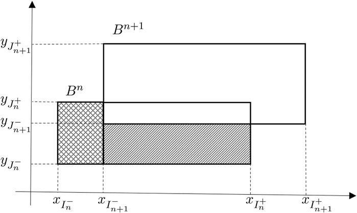
Figure 2. Kinetic domains $B^n$ and $B^{n+1}$ at two successive time steps. The shaded rectangles form the region in Equation 22.

When an agent $i^{\prime }$ crosses an interface and pass from the microscopic domain to the kinetic domain, the agent is added to the probability distribution function $f_{i,j,k}^n$:

$f_{i,j,k}^n\leftarrow f_{i,j,k}^n+E_{R_0}\left({\mathbf{x}}_i-{\mathbf{x}}_{i^{\prime }}\right)E_{R_0}\left(q_j-q_{i^{\prime }}\right)m_{i^{\prime }},$

where $E_{R_0}$ is defined component-wise in Equation 18. This updated $f_{i,j,k}^n$ is plugged into Equation 14 and index $i^{\prime }$ is removed from set $A^n$, so that $A^{n+1}=A^n\backslash \{i^{\prime }\}$.

Next, we consider crossing the interface in the opposite direction, i.e., from the kinetic domain to the microscopic domain. Suppose that $x_{I_{n+1}^{-}}>x_{I_n^{-}}$, $x_{I_{n+1}^{+}}>x_{I_n^{+}}$ and $y_{J_{n+1}^{-}}>y_{J_n^{-}}$, $y_{J_{n+1}^{+}}>y_{J_n^{+}}$, as in Figure 2. Other cases are treated analogously. Then, the following region becomes part of the microscopic domain:

$\left[x_{I_n^{-}},x_{I_{n+1}^{-}}\right]\times \left[y_{J_n^{-}},y_{J_n^{+}}\right]\cup \left[x_{I_{n+1}^{-}},x_{I_n^{+}}\right]\times \left[y_{J_n^{-}},y_{J_{n+1}^{-}}\right].(22)$

This is the union of the shaded rectangles in Figure 2.

We explain the procedure we follow for $[x_{I_n^{-}},x_{I_{n+1}^{-}}]\times [y_{J_n^{-}},y_{J_n^{+}}]$, with the understanding that the same procedure is repeated for $[x_{I_{n+1}^{-}},x_{I_n^{+}}]\times [y_{J_n^{-}},y_{J_{n+1}^{-}}]$. Let $I_1$ be the set of indexes $i$ such that $x_i\in [x_{I_n^{-}},x_{I_{n+1}^{-}}]$ and $J_1$ be the set of indexes $j$ such that $y_i\in [y_{J_n^{-}},y_{J_n^{+}}]$. The mass of people that occupy a position in $[x_{I_n^{-}},x_{I_{n+1}^{-}}]\times [y_{J_n^{-}},y_{J_n^{+}}]$, which belongs to the microscopic domain at time $t^{n+1}$, is given by:

${\displaystyle \sum _{i\in I_1}}{\displaystyle \sum _{j\in J_1}}{\displaystyle \sum _k}{f}_{i,j,k}^n|{\mathrm{\Omega }}_{i,j}|\mathrm{\Delta }q.(23)$

Hence, we create a new agent $i^{\prime }$ at the midpoint of $[x_{I_n^{-}},x_{I_{n+1}^{-}}]\times [y_{J_n^{-}},y_{J_n^{+}}]$, with mass equal Equation 23 for conservation and fear level equal to the average fear level in $[x_{I_n^{-}},x_{I_{n+1}^{-}}]\times [y_{J_n^{-}},y_{J_n^{+}}]$:

$\begin{array}{ll}\hfill & x_{i^{\prime }}^n=\frac{1}{2}\left(x_{I_n^{-}}^n+x_{I_{n+1}^{-}}^n\right),y_{i^{\prime }}^n=\frac{1}{2}\left(y_{J_n^{-}}+y_{J_n^{+}}\right),m_{i^{\prime }}^n={\displaystyle \sum _{i\in I_1}}{\displaystyle \sum _{j\in J_1}}{\displaystyle \sum _k}{f}_{i,j,k}^n|{\mathrm{\Omega }}_{i,j}|\mathrm{\Delta }q,\hfill \\ \hfill & q_{i^{\prime }}^n=\frac{{\sum }_{i\in I_1}{\sum }_{j\in J_1}{\sum }_k{q}_k{f}_{i,j,k}^n|{\mathrm{\Omega }}_{i,j}|\mathrm{\Delta }q}{{\sum }_{i\in I_1}{\sum }_{j\in J_1}{\sum }_k{f}_{i,j,k}^n|{\mathrm{\Omega }}_{i,j}|\mathrm{\Delta }q}.\hfill \end{array}$

Index $i^{\prime }$ gets added to $A^n$ to form $A^{n+1}=A^n\cup \{i^{\prime }\}$. Just like in 1D, if Equation 23 is smaller than 1, a new agent is not created and the position of the interfaces are not changed. However, over a certain number of time steps, the mass leaving the kinetic domain for the microscopic domain will be equal or exceed 1, and then the interface changes.

Let us consider interface $\{x_{I_n^{+}}\}\times [y_{J_n^{-}},y_{J_n^{+}}]$. For simplicity, we assume that $x_{I_n^{+}}$ corresponds to $x_i$ (mesh point) and that ${\theta }_{i,j}$ is positive for all $j$ in $[y_{J_n^{-}},y_{J_n^{+}}]$. The total number of agents leaving the kinetic domain through this interface over time interval $[t^m,t^n]$ equals

${\displaystyle \sum _k}{\displaystyle \sum _{l=m}^n}{\displaystyle \sum _{j\in J_1}}{q}_k\cos {\theta }_{i,j}{f}_{i,j,k}^l\mathrm{\Delta }y\mathrm{\Delta }q\mathrm{\Delta }t.$

When this mass is greater than or equal 1, we create a new agent $j^{\prime }$ with parameters

$\begin{array}{ll}\hfill x_{j^{\prime }}^n& =x_{I_n^{+}}^n,q_{j^{\prime }}^n=\frac{{\sum }_k{\sum }_{l=m}^n{\sum }_{j\in J_1}{\left(q_k\right)}^2\cos {\theta }_{i,j}{f}_{i,j,k}^l\mathrm{\Delta }y\mathrm{\Delta }q\mathrm{\Delta }t}{{\sum }_k{\sum }_{l=m}^n{\sum }_{j\in J_1}{q}_k\cos {\theta }_{i,j}{f}_{x_i,j,k}^l\mathrm{\Delta }y\mathrm{\Delta }q\mathrm{\Delta }t},\hfill \\ \hfill m_{j^{\prime }}^n& ={\displaystyle \sum _k}{\displaystyle \sum _{l=m}^n}{\displaystyle \sum _{j\in J_1}}{q}_k\cos {\theta }_{i,j}{f}_{i,j,k}^l\mathrm{\Delta }y\mathrm{\Delta }q\mathrm{\Delta }t,\hfill \end{array}$

and $y_{j^{\prime }}^n$ is randomly chosen from the interval $[y_{J_n^{-}},y_{J_n^{+}}]$. A similar computation is performed at the interface $[x_{I_n^{-}},x_{I_n^{+}}]\times \{y_{J_n^{+}}\}$.

In conclusion, at time $t^{n+1}$ for all agents $i\in A^{n+1}$ in the microscopic domain, position and fear level are given by Equation 12, the mass is computed as explained above, and the average fear level q_i*^,n is computed by

$q_i^{*,n}=\frac{{\sum }_{l\in A^n}\kappa \left(|\left({\mathbf{x}}_l^n-{\mathbf{x}}_i^n|\right)m_l^n{q}_l^n+{\sum }_{\left(i^{\prime },{ȷ}^{\prime }\right)\in B^n}{\sum }_k\kappa \left(|\left(x_{i^{\prime }},y_{j^{\prime }}\right)\right.-\left(x_i^n,y_i^n\right)|\right)q_k{f}_{i^{\prime },j^{\prime },k}^n|{\mathrm{\Omega }}_{i^{\prime },j^{\prime }}|\mathrm{\Delta }q}{{\sum }_{l\in A^n}\kappa \left(|\left({\mathbf{x}}_l^n-{\mathbf{x}}_i^n|\right)m_l^n+{\sum }_{\left(i^{\prime },j^{\prime }\right)\in B^n}{\sum }_k\kappa \left(|\left(x_{i^{\prime }},y_{j^{\prime }}\right)\right.-\left(x_i^n,y_i^n\right)|\right)f_{i^{\prime },j^{\prime },k}^n|{\mathrm{\Omega }}_{i^{\prime },j^{\prime }}|\mathrm{\Delta }q}.$

For the cells that belong to the kinetic domain $B^n=[x_{I_{n+1}^{-}},x_{I_{n+1}^{+}}]\times [y_{J_{n+1}^{-}},y_{J_{n+1}^{+}}]$, the values of the probability distribution function $f_{j,k,l}^{n+1}$ are given by scheme Equation 14. At a mesh point $(x_i,y_j)$ of the kinetic domain, the average fear level q_i,j*^,n is computed by:

$q_{i,j}^{*,n}=\frac{{\sum }_{l\in A^n}\kappa \left(|{\mathbf{x}}_l^n-{\mathbf{x}}_i^n|\right)m_l^n{q}_l^n+{\sum }_{\left(i^{\prime },j^{\prime }\right)\in B^n}{\sum }_k\kappa \left(|\left(x_{i^{\prime }},y_{j^{\prime }}\right)-\left(x_i,y_j\right)|\right)q_k{f}_{i^{\prime },j^{\prime },k}^n|{\mathrm{\Omega }}_{i^{\prime },j^{\prime }}|\mathrm{\Delta }q}{{\sum }_{l\in A^n}\kappa \left(|{\mathbf{x}}_l^n-{\mathbf{x}}_i^n|\right)m_l^n+{\sum }_{\left(i^{\prime },j^{\prime }\right)\in B^n}{\sum }_k\kappa \left(|\left(x_{i^{\prime }},y_{j^{\prime }}\right)-\left(x_i,y_j\right)|\right)f_{i^{\prime },j^{\prime },k}^n|{\mathrm{\Omega }}_{i^{\prime },j^{\prime }}|\mathrm{\Delta }q}.$

4 Numerical results

We assess our hybrid method through test cases in one dimension, presented in Section 4.1, and two dimensions, reported in Section 4.2.

4.1 Tests in one dimension

We consider $N=1000$ agents that are initially uniformly distributed on the computational domain $[-\mathrm{50,50}]$, so we have an initial uniform density of 10. We initially set the fear level of the agents in the interval $[-\mathrm{50,0}]$ to be equal to 1 and the fear level of the agents in the interval $[\mathrm{0,50}]$ to be 0. This is an unlikely but challenging case where half of the people in the domain have no fear, and thus do not walk, while the remaining half behind them is panicking and hence getting in motion with maximum walking speed. We recall that everyone walks with a direction aligned with the positive $x$-axis. We set the strength of fear contagion $\gamma =1$ and the interaction radius $R=0.1$ in Equation 3. The time interval of interest is [0,4].

The agent based dynamics is obtained via the 1D counterpart of Equation 12 with $\mathrm{\Delta }t=10^{-3}$. Figure 3 shows the plots of the agent density

$\rho \left(x,t\right)={\displaystyle \sum _i}E\left(x-x_i\left(t\right)\right),$

and the average fear level

$q\left(x,t\right)=\frac{{\sum }_i{q}_i\left(t\right)E\left(x-x_i\left(t\right)\right)}{{\sum }_{i}E\left(x-x_i\left(t\right)\right)},$

with $E(x)$ defined in Equation 16 and $r=0.3$, over a part of the computational domain at different times. We see that a region of high density develops near the center of the domain and it propagates to the right.

Figure 3

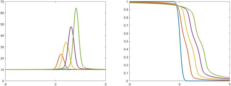
Figure 3. The density of agents (left) and the average fear level (right) from the microscopic model at times $t=0$ (blue) $t=1$ (orange) $t=2$ (yellow), $t=3$ (purple), and $t=4$ (green) over $x\in [-\mathrm{5,5}]$.

Next, we apply the hybrid microscopic-kinetic methods from Section 3.1, with critical density ${\rho }_c=15$. As can be seen from Figure 3, initially we have $\rho <{\rho }_c$ everywhere. Thus, our approach starts with the agent-based model everywhere in $[-\mathrm{50,50}]$. Then, as time passes, $\rho$ becomes larger than ${\rho }_c$ over part of the domain. This is when our approach becomes indeed hybrid, with the kinetic domain moving to the right as time evolves. We consider 4 different meshes with mesh size $\mathrm{\Delta }x=\mathrm{\Delta }y=\mathrm{\Delta }q=0.025$ and the time step is set according to Equation 13. We start with the first order numerical scheme, i.e., no limiter is used. Figure 4 compares the crowd density obtained by the hybrid scheme with the density given by the microscopic model at the end of the time interval of interest, i.e., at $t=4$. We see that for coarser meshes the results given by hybrid model and the microscopic model differ significantly. However, when the mesh is refined the densities computed by the 2 methods become closer and closer, as one would expect.

Figure 4

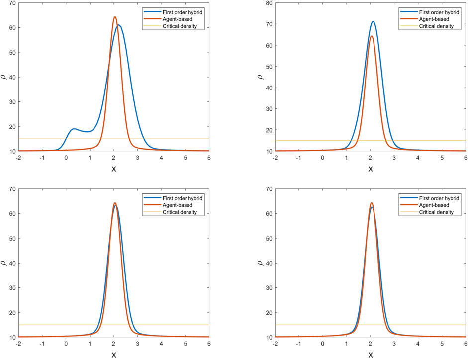
Figure 4. Crowd density given by the microscopic model and the first order hybrid method with meshes $\mathrm{\Delta }x=\mathrm{\Delta }q=0.1$ (top, left), $\mathrm{\Delta }x=\mathrm{\Delta }q=0.05$ (top, right), $\mathrm{\Delta }x=\mathrm{\Delta }q=0.025$ (bottom, left), and $\mathrm{\Delta }x=\mathrm{\Delta }q=0.0125$ (bottom, right) at $t=4$.

Now, let us consider the same meshes and time steps as above, with the second-order scheme. Figures 5, 6 show the crowd density when the van Leer limiter and the minmod limiter are applied, respectively, and the comparison with the crowd density given by the microscopic model. Again, we see great agreement as the mesh is refined.

Figure 5

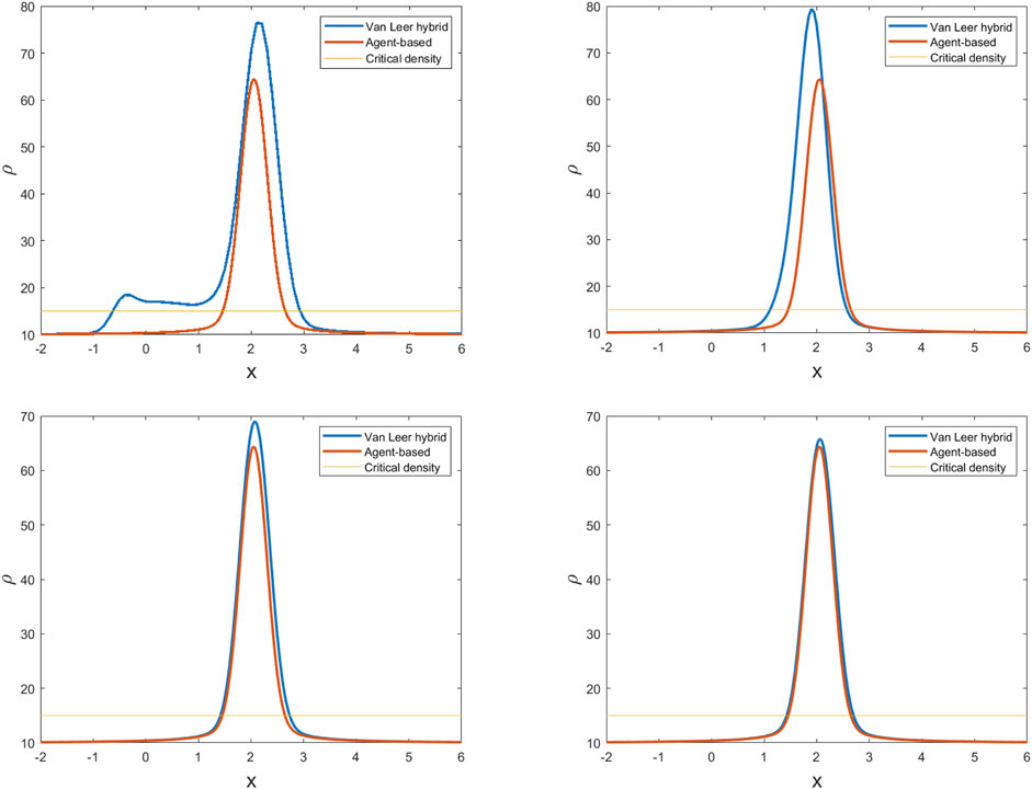
Figure 5. Crowd density given by the microscopic model and the hybrid method with the van Leer limiter and meshes $\mathrm{\Delta }x=\mathrm{\Delta }q=0.1$ (top, left), $\mathrm{\Delta }x=\mathrm{\Delta }q=0.05$ (top, right), $\mathrm{\Delta }x=\mathrm{\Delta }q=0.025$ (bottom, left), and $\mathrm{\Delta }x=\mathrm{\Delta }q=0.0125$ (bottom, right) at time $t=4$.

Figure 6

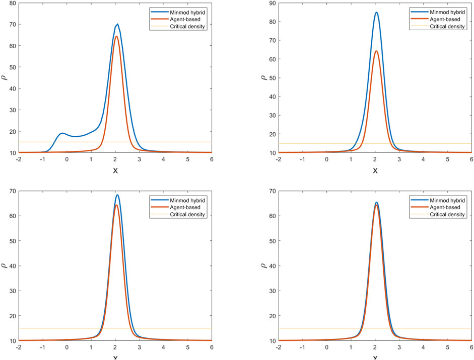
Figure 6. Crowd density given by the microscopic model and the hybrid method with the minmod limiter and meshes $\mathrm{\Delta }x=\mathrm{\Delta }q=0.1$ (top, left), $\mathrm{\Delta }x=\mathrm{\Delta }q=0.05$ (top, right), $\mathrm{\Delta }x=\mathrm{\Delta }q=0.025$ (bottom, left), and $\mathrm{\Delta }x=\mathrm{\Delta }q=0.0125$ (bottom, right) at time $t=4$.

To quantify the comparisons in Figures 4–6 and Tables 1, 2 report the corresponding differences in $L^1$ and $L^2$ norms. From these tables, we see that the second-order schemes perform marginally better than the first-order scheme and are comparable to each other. We notice that this is not a convergence test, as the solution given by the microscopic model cannot be considered the exact solution for the kinetic model. It is just showing that when the crowd is rather dense and the mesh is fine enough, the microscopic model and the hybrid approach are in agreement.

Table 1

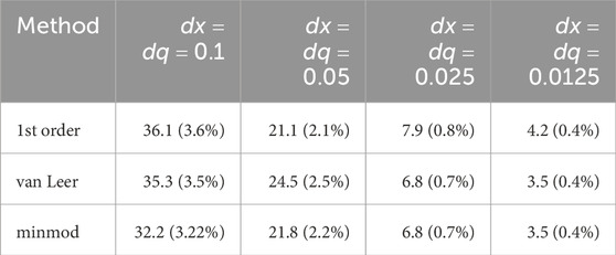
Table 1. Difference between the solution given by the microscopic model and the solution given by the hybrid approaches in $L^1$ norm at time $t=4$, with relative difference included in parenthesis.

Table 2

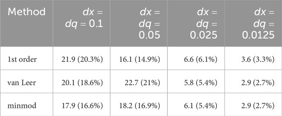
Table 2. Difference between the solution given by the microscopic model and the solution given by the hybrid approaches in $L^2$ norm at time $t=4$, with relative difference included in parenthesis.

Finally, we present some results that show the importance of model parameter $\gamma$. Recall that $\gamma$ in Equation 1 is the interaction strength, i.e., how much an agent is willing to adjust their fear level, and hence walking speed, to equilibrate it with the local average. The results presented thus far were obtained with $\gamma =1$. Figure 7 shows the crowd density given by the hybrid method for $\gamma =0.1,10$ with the minmod limiter. All the other settings are the same used so far. By comparing Figure 7 with Figure 3 (left), we see that the crowd density is very sensitive to the value of $\gamma$, both in terms of magnitude of the peaks and overall distribution.

Figure 7

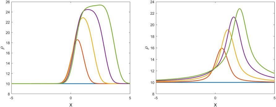
Figure 7. Crowd density given by the hybrid method for $\gamma =0.1$ (left) and $\gamma =10$ (right) with the minmod limiter at times $t=0$ (blue) $t=1$ (orange) $t=2$ (yellow), $t=3$ (purple), and $t=4$ (green) over $x\in [-\mathrm{5,5}]$. The results refer to mesh $\mathrm{\Delta }x=\mathrm{\Delta }q=0.025$.

While constant $\gamma$ is convenient, it is not very realistic since different people react differently to a spreading emotion. Figure 8 reports the results obtained with the microscopic model and random values of $\gamma \in (\mathrm{0,1})$ assigned to the agents, shown in the leftmost panel. Notice how the heterogeneity in the values of $\gamma$ leads to local oscillations in the density (central panel) and average fear level (rightmost panel).

Figure 8

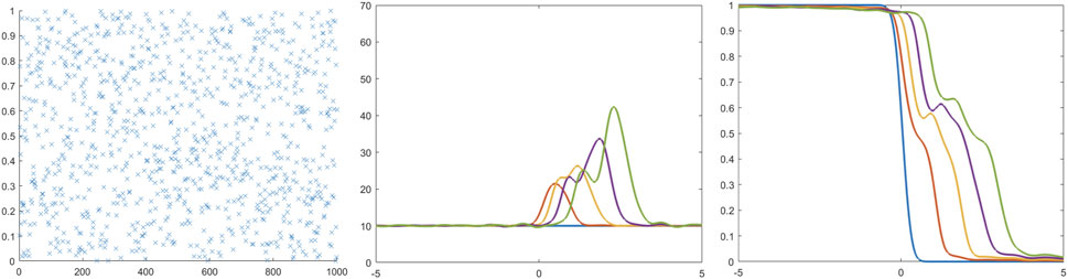
Figure 8. Scatter plot showing the random gamma values for each of 1,000 agents (left), along with corresponding agent density (center) and average fear level (right) given by the microscopic model at times $t=0$ (blue) $t=1$ (orange) $t=2$ (yellow), $t=3$ (purple), and $t=4$ (green).

4.2 Tests in two dimensions

We consider $N=900$ agents initially placed uniformly in computational domain $[-\mathrm{10,10}]\times [-\mathrm{10,10}]$, so that the initial density is equal to 9 everywhere in the domain. The initial fear level is set to 1 inside the circle of radius 3 centered at the origin of the axes, while everywhere else it is set to 0. This set up is meant to reproduce a case where a group of people inside a uniformly dense crowd gets scared (by, e.g., the onset of a fire) and panics, while all other people are not aware of the threat and thus do not move. We assume that all moving agents choose walking direction $\theta =\pi /4$, possibly the direction where an exit is located. We set $\gamma =1$ and $R=0.1$ in Equation 3. The time interval of interest is [0,5].

The agent based dynamics is obtained by using Equation 12 with $\mathrm{\Delta }t=10^{-3}$. Figure 9 shows the plots of the agent density

$\rho \left(\mathbf{x},t\right)={\displaystyle \sum _i}E\left(\mathbf{x}-{\mathbf{x}}_i\left(t\right)\right),$

and the average fear level

$q\left(\mathbf{x},t\right)=\frac{{\sum }_i{q}_i\left(t\right)E\left(\mathbf{x}-{\mathbf{x}}_i\left(t\right)\right)}{{\sum }_{i}E\left(\mathbf{x}-{\mathbf{x}}_i\left(t\right)\right)}$

at $t=\mathrm{4,4.5},5$, with $E(x)$ defined component-wise in Equation 16 and $r=0.3$.

Figure 9

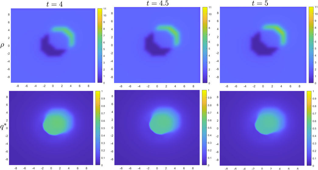
Figure 9. The density of agents (top row) and average fear level (bottom row) given by the microscopic model at times $t=4$ (left), $t=4.5$ (center), and $t=5$ (right).

Next, we apply the hybrid microscopic-kinetic methods from Section 3.2, with critical density ${\rho }_c=4$. Since initially $\rho <{\rho }_c$ everywhere in the domain, our scheme starts with the microscopic model everywhere. As time passes, $\rho$ becomes larger than ${\rho }_c$ over parts of the domain and our approach becomes truly hybrid. We consider 3 different meshes with mesh size $\mathrm{\Delta }x=\mathrm{\Delta }y=\mathrm{\Delta }q=0.25,0.125,0.0625$. The time step is set according to Equation 13. We start with the first order numerical scheme, i.e., no limiter is used. Figure 10 compares the crowd density obtained by the microscopic model (top left panel) with the density computed by the hybrid approach with the three meshes under consideration at time $t=5$. As in the one-dimensional case, the results from the hybrid and microscopic models differ significantly when a coarse mesh is used. However, as the mesh is refined, the densities computed by the two methods become increasingly closer.

Figure 10

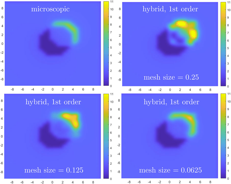
Figure 10. Crowd density given by the microscopic model (top, left) and first order hybrid method with meshes $\mathrm{\Delta }x=\mathrm{\Delta }y=\mathrm{\Delta }q=0.25$ (top, right), $\mathrm{\Delta }x=\mathrm{\Delta }y=\mathrm{\Delta }q=0.125$ (bottom, left), and $\mathrm{\Delta }x=\mathrm{\Delta }y=\mathrm{\Delta }q=0.0625$ (bottom, right) at $t=5$.

We repeat the comparison using a second-order schemes, with the same meshes and time step as above. Figures 11, 12 report the microscopic vs. hybrid comparison in terms of crowd density when the van Leer limiter and the minmod limiter are applied, respectively. Again, we see that the agreement improves as the computational mesh is refined.

Figure 11

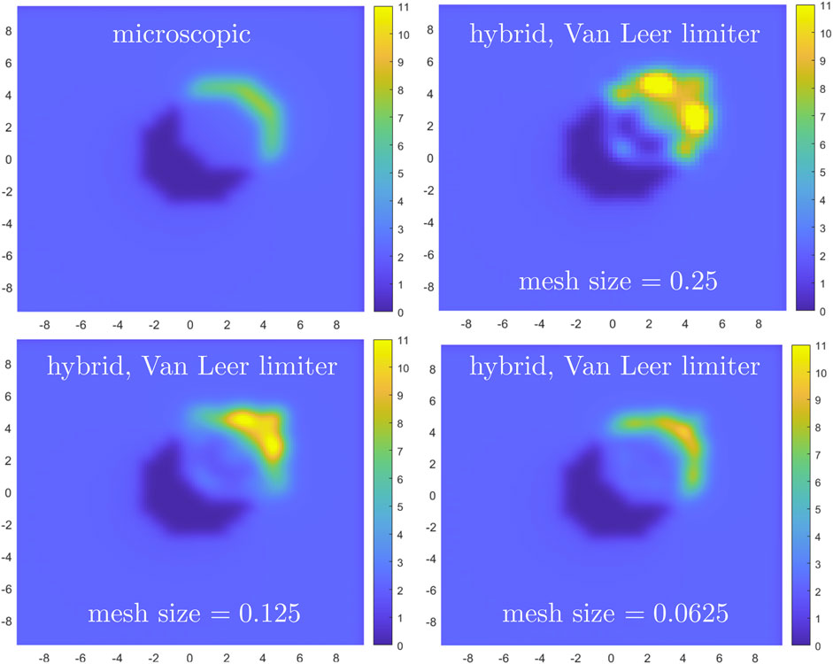
Figure 11. Crowd density given by the microscopic model (top, left) and the hybrid method with the Van Leer limiter scheme for meshes $\mathrm{\Delta }x=\mathrm{\Delta }y=\mathrm{\Delta }q=0.25$ (top, right), $\mathrm{\Delta }x=\mathrm{\Delta }y=\mathrm{\Delta }q=0.125$ (bottom, left), and $\mathrm{\Delta }x=\mathrm{\Delta }y=\mathrm{\Delta }q=0.0625$ (bottom, right) at $t=5$.

Figure 12

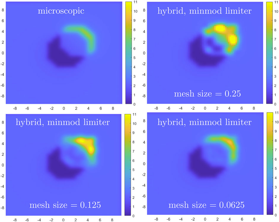
Figure 12. Crowd density given by the microscopic model (top, left) and the hybrid method with the minmod limiter scheme for meshes $\mathrm{\Delta }x=\mathrm{\Delta }y=\mathrm{\Delta }q=0.25$ (top, right), $\mathrm{\Delta }x=\mathrm{\Delta }y=\mathrm{\Delta }q=0.125$ (bottom, left), and $\mathrm{\Delta }x=\mathrm{\Delta }y=\mathrm{\Delta }q=0.0625$ (bottom, right) at $t=5$.

To quantify the level of agreement shown in Figures 10–12, we report in Tables 3, 4 the difference in absolute value between the solution given by the microscopic model and the solution given by the hybrid approach in the $L^1$ and $L^2$ norms. In this comparison, which we recall is not a convergence test, we do not observe a significant difference when using limiters compared to the first-order scheme. Like in the 1D case, we see that when the crowd is rather dense and the mesh is fine enough, the microscopic model and the hybrid approach are in agreement.

Table 3

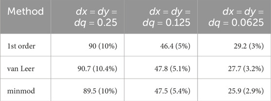
Table 3. Difference in absolute value between the solution given by the microscopic model and the solution given by the hybrid approaches in the $L^1$ norm at time $T=5$, with relative difference included in parenthesis.

Table 4

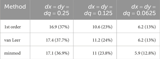
Table 4. Difference in absolute value between the solution given by the microscopic model and the solution given by the hybrid approaches in the $L^2$ norm at time $T=5$, with relative difference included in parenthesis.

We conclude by considering the more realistic case where the value of the interaction strength varies from one agent to the other. Like for the corresponding 1D test, we assign a random value of $\gamma$ in interval (0,1) to each agent. See the assigned values in Figure 13. Figure 14 reports the crowd density and average fear level at $t=\mathrm{4,4.5},5$ obtained with the microscopic model and these random values of $\gamma$. In both quantities, we observe local oscillations that were absent when the value of $\gamma$ was constant in space (see Figure 9).

Figure 13

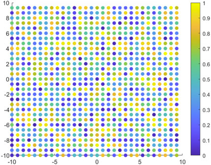
Figure 13. Random values of $\gamma$ for each of the 900 agents.

Figure 14

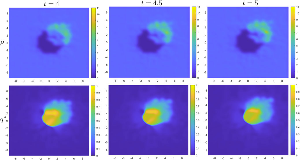
Figure 14. Crowd density (top row) and average fear level (bottom row) given by the microscopic model with the values of $\gamma$ shown in Figure 13 at times $t=4$ (left), $t=4.5$ (center), and $t=5$ (right).

5 Conclusions and future perspectives

We developed and numerically analyzed a hybrid modeling approach for simulating crowd dynamics under the influence of propagating fear in walking venues with mixed crowd densities. The hybrid nature is related to the fact that our approach uses a microscopic (agent-based) model in low-density regions, while in higher-density areas it adopts a mesoscopic (kinetic) model, derived from the microscopic model via a mean-field limit approach. The microscopic model captures individual variability and local interactions, while the mesoscopic model efficiently handles collective behaviors in denser crowds. By coupling the two models with appropriate interface conditions, we take advantages of their strengths while mitigating their respective limitations. We ensured consistency between the two models through a mean-field limit and proposed interface conditions to enable seamless coupling of regions of varying density.

We performed tests in one and two dimensional spatial domains. We showed that our hybrid approach produces results in agreement with those provided by the microscopic model when the crowd is sufficiently dense and the computational mesh is fine enough. This validates the effectiveness of our hybrid strategy in accurately capturing crowd dynamics across varying density regimes. Additionally, our tests demonstrate the sensitivity of the computed crowd density and average fear level on model parameter $\gamma$, which controls the strength of emotional interactions. Thus, one would have to find a way to carefully set this parameter to realistically simulate crowd responses in fear-driven scenarios.

In order to focus on the behavioral features of crowd dynamics, we have introduced a strong simplification in this work: the walking direction is prescribed. This choice represents the main limitation of the hybrid model presented in this paper. In reality, each individual in a crowd has their own purposes and abilities, which lead to the selection of a walking strategy, i.e., a trajectory to follow in order to reach the desired target(s) and a speed to move along such trajectory. The walking strategy is influenced by the emotional state (considered in this paper) and the interactions with other people in the crowd and the environment, which includes walls, exits, and obstacles (not considered in this paper). A relatively easy way to account for such interactions is with tools of game theory, as we have done in [18, 23]. However, the resulting more realistic model presents difficulties at the numerical level related to need to contain high computational costs. One possible way to meet this need is through splitting algorithms, which break the model into a set of subproblems that are easier to solve and for which practical algorithms are readily available. The inclusion of interactions with people and the environment and the development of suitable splitting algorithms will be object of future work.

Data availability statement

The raw data supporting the conclusions of this article will be made available by the authors upon request, without undue reservation.

Author contributions

IP: Validation, Writing – original draft, Visualization, Methodology, Formal Analysis, Investigation, Software, Writing – review and editing. AQ: Conceptualization, Investigation, Methodology, Supervision, Writing – review and editing, Writing – original draft.

Funding

The author(s) declare that no financial support was received for the research and/or publication of this article.

Conflict of interest

The authors declare that the research was conducted in the absence of any commercial or financial relationships that could be construed as a potential conflict of interest.

Generative AI statement

The author(s) declare that no Generative AI was used in the creation of this manuscript.

Publisher’s note

All claims expressed in this article are solely those of the authors and do not necessarily represent those of their affiliated organizations, or those of the publisher, the editors and the reviewers. Any product that may be evaluated in this article, or claim that may be made by its manufacturer, is not guaranteed or endorsed by the publisher.

References

1. Helbing D, Johansson A, Al-Abideen HZ. Dynamics of crowd disasters: an empirical study. Phys Rev E (2007) 75:046109. doi:10.1103/PhysRevE.75.046109

PubMed Abstract | CrossRef Full Text | Google Scholar

2. Helbing D, Johansson A. Pedestrian, crowd, and evacuation dynamics. New York, NY: Springer New York (2009). p. 1–28. doi:10.1007/978-3-642-27737-5_382-5

CrossRef Full Text | Google Scholar

3. Wijermans N, Conrado C, van Steen M, Martella C, Li J. A landscape of crowd-management support: an integrative approach. Saf Sci (2016) 86:142–64. doi:10.1016/j.ssci.2016.02.027

CrossRef Full Text | Google Scholar

4. Haghani M, Sarvi M. Social dynamics in emergency evacuations: disentangling crowd’s attraction and repulsion effects. Physica A: Stat Mech its Appl (2017) 475:24–34. doi:10.1016/j.physa.2017.02.010

CrossRef Full Text | Google Scholar

5. Aylaj B, Bellomo N, Gibelli L, Reali A. A unified multiscale vision of behavioral crowds. Math Models Methods Appl Sci (2020) 30(1):1–22. doi:10.1142/s0218202520500013

CrossRef Full Text | Google Scholar

6. Bellomo N, Gibelli L, Quaini A, Reali A. Towards a mathematical theory of behavioral human crowds. Math Models Methods Appl Sci (2022) 32(02):321–58. doi:10.1142/s0218202522500087

CrossRef Full Text | Google Scholar

7. Bellomo N, Liao J, Quaini A, Russo L, Siettos C. Human behavioral crowds review, critical analysis and research perspectives. Math Models Methods Appl Sci (2023) 33(08):1611–59. doi:10.1142/s0218202523500379

CrossRef Full Text | Google Scholar

8. Helbing D, Farkas I, Vicsek T. Simulating dynamical features of escape panic. Natures (2000) 407:487–90. doi:10.1038/35035023

PubMed Abstract | CrossRef Full Text | Google Scholar

9. Wang J, Zhang L, Shi Q, Yang P, Hu X. Modeling and simulating for congestion pedestrian evacuation with panic. Physica A: Stat Mech its Appl (2015) 428:396–409. doi:10.1016/j.physa.2015.01.057

CrossRef Full Text | Google Scholar

10. Zou Y, Xie J, Wang B. Evacuation of pedestrians with two motion modes for panic system. PLoS One (2016) 11(4):e0153388. doi:10.1371/journal.pone.0153388

PubMed Abstract | CrossRef Full Text | Google Scholar

11. Rahmati Y, Talebpour A. Learning-based game theoretical framework for modeling pedestrian motion. Phys Rev E (2018) 98:032312. doi:10.1103/PhysRevE.98.032312

CrossRef Full Text | Google Scholar

12. Xu M, Xie X, Lv P, Niu J, Wang H, Li C, et al. Crowd behavior simulation with emotional contagion in unexpected multihazard situations. IEEE Trans Syst Man, Cybernetics: Syst (2021) 51(3):1–15. doi:10.1109/TSMC.2019.2899047

CrossRef Full Text | Google Scholar

13. van Haeringen E, Gerritsen C, Hindriks K. Emotion contagion in agent-based simulations of crowds: a systematic review. Auton Agent Multi-agent Syst (2023) 37:6. doi:10.1007/s10458-022-09589-z

CrossRef Full Text | Google Scholar

14. Bellomo N, Bellouquid A. On multiscale models of pedestrian crowds from mesoscopic to macroscopic. Commun Math Sci (2015) 13:1649–64. doi:10.4310/cms.2015.v13.n7.a1

CrossRef Full Text | Google Scholar

15. Bellomo N, Bellouquid A, Gibelli L, Outada N. A quest towards a mathematical theory of living systems. In: Modeling and simulation in science, engineering and technology. Birkhäuser (2017). doi:10.1007/978-3-319-57436-3

CrossRef Full Text | Google Scholar

16. Bellomo N, Gibelli L. Toward a mathematical theory of behavioral-social dynamics for pedestrian crowds. Math Models Methods Appl Sci (2015) 25(13):2417–37. doi:10.1142/S0218202515400138

CrossRef Full Text | Google Scholar

17. Bellomo N, Gibelli L, Outada N. On the interplay between behavioral dynamics and social interactions in human crowds. Kinetic Relat Models (2019) 12(2):397–409. doi:10.3934/krm.2019017

CrossRef Full Text | Google Scholar

18. Kim D, Quaini A. A kinetic theory approach to model pedestrian dynamics in bounded domains with obstacles. Kinetic Relat Models (2019) 12(6):1273–96. doi:10.3934/krm.2019049

CrossRef Full Text | Google Scholar

19. Wang L, Short MB, Bertozzi AL. Efficient numerical methods for multiscale crowd dynamics with emotional contagion. Math Models Methods Appl Sci (2017) 27(1):205–30. doi:10.1142/S0218202517400073

CrossRef Full Text | Google Scholar

20. Llorca D, Haghani M, Cristiani E, Bode N, Boltes M, Corbetta A. Panic, irrationality, and herding: three ambiguous terms in crowd dynamics research. J Adv Transportation (2019) 2019:1–58. doi:10.1155/2019/9267643

CrossRef Full Text | Google Scholar

21. Bellomo N, Bellouquid A, Knopoff D. From the microscale to collective crowd dynamics. SIAM Multiscale Model and Simulation (2013) 11(3):943–63. doi:10.1137/130904569

CrossRef Full Text | Google Scholar

22. Agnelli JP, Colasuonno F, Knopoff D. A kinetic theory approach to the dynamics of crowd evacuation from bounded domains. Math Models Methods Appl Sci (2015) 25(01):109–29. doi:10.1142/S0218202515500049

CrossRef Full Text | Google Scholar

23. Kim D, O’Connell K, Ott W, Quaini A. A kinetic theory approach for 2D crowd dynamics with emotional contagion. Math Models Methods Appl Sci (2021) 31(06):1137–62. doi:10.1142/S0218202521400030

CrossRef Full Text | Google Scholar

24. Kim D, Labate D, Mily K, Quaini A. Data-driven learning to enhance a kinetic model of distressed crowd dynamics. Math Models Methods Appl Sci (2025) 35(07):1609–36. doi:10.1142/S021820252540007X

CrossRef Full Text | Google Scholar

25. Bakhdil N, El Mousaoui A, Hakim A. A kinetic BGK model for pedestrian dynamics accounting for anxiety conditions. Symmetry (2025) 17(1):19. doi:10.3390/sym17010019

CrossRef Full Text | Google Scholar

26. LeVeque RJ. Numerical methods for conservation laws. In: Lectures in mathematics, ETH Zürich. Basel: Birkhäuser Verlag (1990).

Google Scholar