Distributed-order -deformed Lévy processes and their spectral properties

Lévy processes play a central role in stochastic modeling, providing a unifying framework for jump dynamics, anomalous diffusion, and heavy-tailed phenomena across physics and applied sciences. We propose a novel framework for $(q,\tau ,\alpha ,\beta )$-generalized Lévy processes, extending fractional and tempered stable models with $(q,\tau )$-Gamma and $(q,\tau )$-Mittag--Leffler functions. The construction uses Laplace transforms of $(q,\tau )$-inverse subordinators combined with the Lévy--Khintchine representation to obtain explicit expressions for characteristic functions. Numerical results show how variations in $q$ and $\tau$ affect ${\mathrm{\Gamma }}_{q,\tau }(x)$ and $E_{\beta }^{(q,\tau )}(z)$, leading to slower relaxation, heavier tails, and enhanced memory effects relative to classical counterparts. These outcomes demonstrate that $(q,\tau )$-deformation provides a flexible mechanism for modeling anomalous diffusion, nonlocal dynamics, and heavy-tailed processes relevant in physics, finance, and geophysics.

1 Introduction

For simulating a wide range of complicated events with heavy tails, memory effects, and nonlocal interactions, L’evy processes and their fractional generalizations have become essential tools. Applications include biological systems displaying LEvy flight behavior [1–4], financial time series containing extreme events, and anomalous transport in physics and turbulent flows. The Lévy–Khintchine expression, which links the process generator to its characteristic exponent and the underlying Lévy measure, is the foundation of the classical theory of Lévy processes [5–7, 9]. By adding operators of non-integer order, fractional L’evy processes expand this framework and produce multi-scaling behavior and rich nonlocal dynamics [8–10].

New tools for fractional modeling have recently been made available by generalized families of special functions that arise in quantum calculus [11–13]. The quantum Gamma function [14, 15] is another name for the $(q,\tau )$-Gamma function, which in particular makes it possible to create $(q,\tau )$-deformed analogues of classical fractional operators. Memory and tempering effects that are absent from conventional fractional models are introduced by these operators, which combine fractional scaling and deformation effects controlled by the parameters $q$ and $\tau$. The temporal development of the associated distorted processes is provided by $(q,\tau )$-Mittag-Leffler functions, which naturally emerge as solutions of $(q,\tau )$-fractional differential equations in this context [16–18]. By combining these tools, it is possible to formulate $(q,\tau )$-deformed Lévy processes with tunable spectral properties and more flexible generators. The inclusion of distributed-order models, in which the fractional order $\alpha$ is not set but rather distributed according to a measure, is a significant extension of this concept. It has been demonstrated that complicated systems with heterogeneous scaling, including biological transport processes, porous media, and viscoelastic materials, may be modeled using distributed-order fractional dynamics.

This paper aims to create and analyze distributed-order $(q,\tau )$-deformed Lévy processes, to examine their spectral features, and to formally identify their generators. Our attention is specifically directed towards the scaling coefficient $K_{q,\tau }^{(\alpha ,\beta )}$, which regulates the interaction between memory, scaling, and deformation effects and governs the spectral behavior of the generators in Fourier space. Through numerical comparisons with both the asymptotic and exact behavior of $K_{q,\tau }^{(\alpha ,\beta )}$ across different regimes, we validate the theoretical results, prove important properties of the generators, and provide a rigorous analysis of the corresponding $(q,\tau )$-Gamma and $(q,\tau )$-Mittag-Leffler functions. For a variety of physics applications, the suggested framework provides a versatile and physically validated extension of Lévy-based models.

2 Objectives and applications of the study

The fundamental objective of this work is to formulate and analyze a new class of stochastic processes driven by distributed-order $(q,\tau )$-deformed fractional dynamics. These approaches enhance typical time-fractional Lévy models by adding fractional orders $\alpha ,\beta >0$, $\tau >0$, and deformation parameters $q\in (\mathrm{0,1})$. These characteristics collectively represent jump heterogeneity, memory, and scaling asymmetry. By proposing the $(q,\tau )$-Lévy-Khintchine exponent and showing that the Laplace transform of the process is governed by a deformed Mittag-Leffler function, the research extends the concept of temporal subordination in fractional stochastic mathematical modeling.

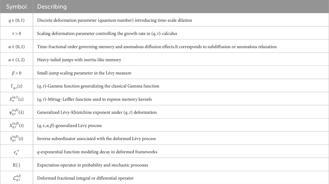
This approach is primarily inspired by complex systems that exhibit multiscale and nonlocal behavior. Applications of the proposed paradigm can be found in many scientific domains. In quantum physics, the $(q,\tau )$-deformation captures algebraic structures related to quantum model phenomena, such as fractional tunneling and memory-driven decoherence. In materials research, the technique can be used for anomalous diffusion in porous or disordered media. In financial mathematics, the memory kernels and flexible jump structure are helpful for simulating large tails and volatility clustering. The model also considers spatial memory, various tissue interactions, and delays in biomedical transport and bio-imaging. Finally, in control and signal processing, the deformed kernel is used as a foundation for adaptive control methods, memory-tuned responses, and nonlocal filtering. These wide-ranging uses validate the $(q,\tau )$-fractional Lévy framework’s adaptability and originality. The summary of the model symbolic is in Table 1.

Table 1

Table 1. Summary of notations utilized in the study.

3 Generalized Time-Fractional Lévy Process

Let $L(t)$ be a Lévy process with Laplace exponent $\psi (\lambda )$. The time-fractional Lévy process $X^{(\alpha )}(t)$ is defined by:

$\mathbb{E}\left[e^{-\lambda X^{\left(\alpha \right)\left(t\right)}}\right]=E_{\alpha }\left(-t^{\alpha }\psi \left(\lambda \right)\right),$

where $E_{\alpha }(\cdot )$ is the one-parameter Mittag–Leffler function:

$E_{\alpha }\left(z\right)≔{\displaystyle \sum _{k=0}^{\infty }}\frac{z^k}{\mathrm{\Gamma }\left(\alpha k+1\right)}.$

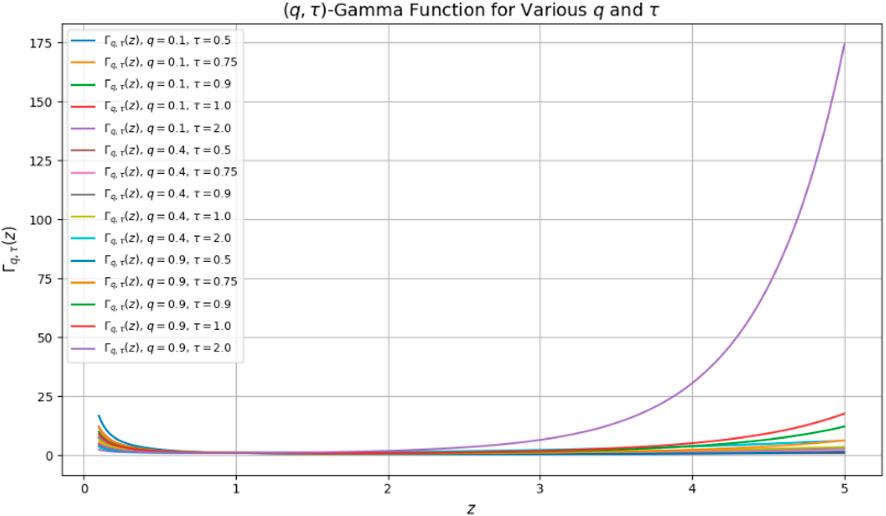
Definition 3.1. The $(q,\tau )$-Gamma function is defined as (see Figure 1):

${\mathrm{\Gamma }}_{q,\tau }\left(z\right)≔{\left(1-q\right)}^{1-z}\prod _{n=0}^{\infty }\frac{1-q^{\tau \left(n+1\right)}}{1-q^{\tau \left(n+z\right)}},0<q<1,\tau >0.$

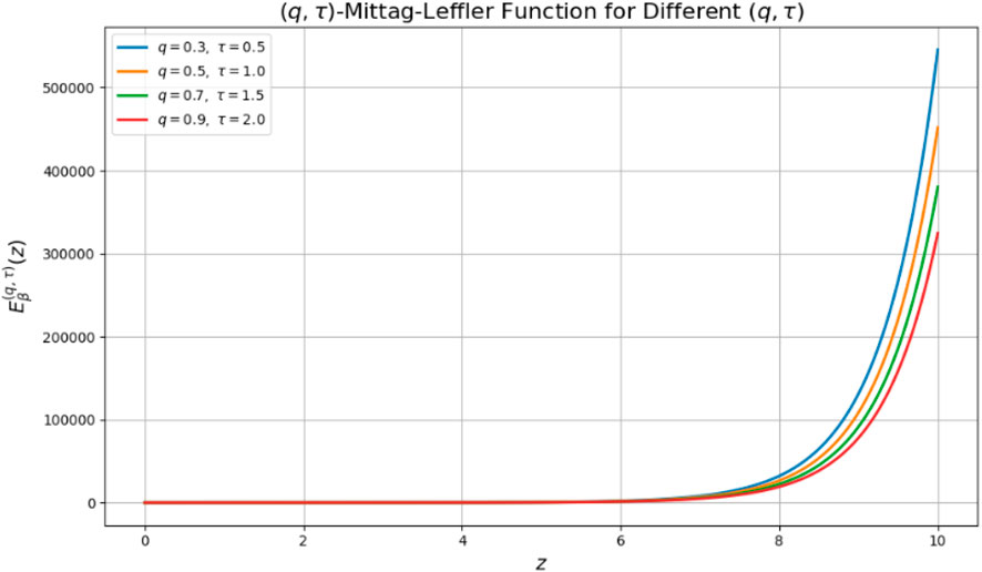
The associated $(q,\tau )$-Mittag–Leffler function is given by (see Figure 2):

$E_{\beta }^{\left(q,\tau \right)}\left(z\right)≔{\displaystyle \sum _{k=0}^{\infty }}\frac{z^k}{{\mathrm{\Gamma }}_{q,\tau }\left(\beta k+1\right)}.$

Figure 1

Figure 1. The graph of the $(q,\tau )$-Gamma function ${\mathrm{\Gamma }}_{q,\tau }(x)$ illustrates how the deformation parameters $q$ and $\tau$ modify the growth pattern of the classical gamma function. The curve corresponds with $\mathrm{\Gamma }(x)$ for $q=1,\tau =1$, however for big $x$, $q<1$ introduces a damping effect that delays divergence, improving memory in fractional kernels. As a scaling factor, the parameter $\tau$ amplifies the damping while $\tau >1$ somewhat accelerates growth. These deformations directly affect waiting-time distributions and tail behavior in fractional L’evy process models, offering a customizable equilibrium between decay rate and memory durability.

Figure 2

Figure 2. In contrast to the classical example, the graph of the $(q,\tau )$-Mittag–Leffler function $E_{\beta }^{(q,\tau )}(z)$ for $\beta =0.9$ illustrates how $(q,\tau )$-deformation modifies the decay profile. Stronger memory effects in the underlying fractional dynamics are reflected in the function’s slower decline when $q<1$. This behavior is modulated by the parameter $\tau$: $\tau >1$ somewhat speeds up the decay rate, but $\tau <1$ increases persistence. These effects give $(q,\tau )$-fractional Lévy-type processes a versatile way to adjust their relaxation behavior.

Proposition 3.2. Let $0<q<1$, $\tau >0$, and $\beta >0$. The $(q,\tau )$-Gamma function is defined as:

${\mathrm{\Gamma }}_{q,\tau }\left(\beta \right)={\left(1-q\right)}^{1-\beta }\cdot \frac{{\left(q^{\tau };q\right)}_{\infty }}{{\left(q^{\tau +\beta };q\right)}_{\infty }},(1)$

where ${(a;q)}_{\infty }={\prod }_{k=0}^{\infty }(1-a{q}^k)$ is the $q$-Pochhammer symbol. The following properties hold:

1. Classical limit. As $\tau \to 1,q\to 1^{-}$, one has:

${\mathrm{\Gamma }}_{q,\tau }\left(\beta \right)\to \mathrm{\Gamma }\left(\beta \right).$

2. Scaling behavior in $\tau$. For fixed $q<1$, the dependence on $\tau$ satisfies:

${\mathrm{\Gamma }}_{q,\tau }\left(\beta \right)={\mathrm{\Gamma }}_{q,1}\left(\beta \right)\cdot \prod _{k=0}^{\infty }\frac{1-q^{\tau +k}}{1-q^{\tau +\beta +k}}.$

3. Monotonicity in $\beta$. The function ${\mathrm{\Gamma }}_{q,\tau }(\beta )$ is strictly decreasing in $\beta$.

4. Asymptotic behavior. For large $\tau$, one has:

${\mathrm{\Gamma }}_{q,\tau }\left(\beta \right)\sim {\left(1-q\right)}^{1-\beta }\cdot q^{-\beta \tau }\cdot C_q,$

where $C_q$ is a constant independent of $\tau$.

Proof. (1) Classical limit. It is known (see standard results in $q$-calculus) that:

$\underset{q\to 1^{-}}{\lim }{\left(a;q\right)}_{\infty }=\exp \left(-{\displaystyle \sum _{n=1}^{\infty }}\frac{a^n}{n}\right)={\left(1-a\right)}^{-1}.$

Applying this to ${(q^{\tau };q)}_{\infty }$ and ${(q^{\tau +\beta };q)}_{\infty }$, and using ${(1-q)}^{1-\beta }\to 1$ as $q\to 1^{-}$, we obtain [12].

${\mathrm{\Gamma }}_{q,\tau }\left(\beta \right)\to \mathrm{\Gamma }\left(\beta \right).$

(2) Scaling behavior in $\tau$. From the definition:

${\mathrm{\Gamma }}_{q,\tau }\left(\beta \right)={\left(1-q\right)}^{1-\beta }\cdot \frac{{\left(q^{\tau };q\right)}_{\infty }}{{\left(q^{\tau +\beta };q\right)}_{\infty }}.$

Now, we observe that

$\frac{{\left(q^{\tau };q\right)}_{\infty }}{{\left(q^{\tau +\beta };q\right)}_{\infty }}=\prod _{k=0}^{\infty }\frac{1-q^{\tau +k}}{1-q^{\tau +\beta +k}},$

Which gives the scaling property.

(3) Monotonicity in $\beta$. Each factor in the product:

$\frac{1-q^{\tau +k}}{1-q^{\tau +\beta +k}}$

is a strictly decreasing function of $\beta$, since the denominator increases with $\beta$. Therefore, the entire product decreases with $\beta$, so ${\mathrm{\Gamma }}_{q,\tau }(\beta )$ is decreasing.

(4) Asymptotic behavior. For large $\tau$, we have:

$1-q^{\tau +\beta +k}\approx q^{\tau +\beta +k},$

and similarly for $1-q^{\tau +k}$. Therefore:

$\prod _{k=0}^{\infty }\frac{1-q^{\tau +k}}{1-q^{\tau +\beta +k}}\sim q^{-\beta \tau }\cdot C_q,$

where $C_q$ is a constant independent of $\tau$. The prefactor ${(1-q)}^{1-\beta }$ remains, giving the full asymptotic behavior.

Proposition 3.3. Let $0<q<1$, $\tau >0$, $\beta >0$, and $z\in \mathbb{C}$. The $(q,\tau )$-Mittag-Leffler function is defined as:

$E_{\beta }^{\left(q,\tau \right)}\left(z\right)≔{\displaystyle \sum _{k=0}^{\infty }}\frac{z^k}{{\mathrm{\Gamma }}_{q,\tau }\left(\beta k+1\right)}.(2)$

The following properties hold:

1. Classical limit. As $q\to 1^{-}$, one has:

$E_{\beta }^{\left(q,\tau \right)}\left(z\right)\to E_{\beta }\left(z\right)={\displaystyle \sum _{k=0}^{\infty }}\frac{z^k}{\mathrm{\Gamma }\left(\beta k+1\right)},$

recovering the standard Mittag-Leffler function.

2. Entire function. $E_{\beta }^{(q,\tau )}(z)$ is an entire function of $z$, of order $1/\beta$.

3. Asymptotic behavior. For large $|z|$, one has:

$E_{\beta }^{\left(q,\tau \right)}\left(z\right)\sim \frac{1}{{\mathrm{\Gamma }}_{q,\tau }\left(1-\beta \right)}{z}^{-1},$

along suitable sectors in the complex plane.

4. Monotonicity on ${\mathbb{R}}^{+}$. For $z\ge 0$, $E_{\beta }^{(q,\tau )}(-z)$ is completely monotonic for $0<\beta \le 1$.

Proof. (1) Classical limit. As $q\to 1^{-}$, by Proposition 2 (see previous result), we have:

${\mathrm{\Gamma }}_{q,\tau }\left(\beta k+1\right)\to \mathrm{\Gamma }\left(\beta k+1\right).$

Therefore, the series reduces to the classical Mittag-Leffler function:

$E_{\beta }^{\left(q,\tau \right)}\left(z\right)\to E_{\beta }\left(z\right).$

(2) Entire function. The radius of convergence $R$ is infinite because:

$\underset{k\to \infty }{\lim }\left|\frac{z^{k+1}}{{\mathrm{\Gamma }}_{q,\tau }\left(\beta \left(k+1\right)+1\right)}\cdot \frac{{\mathrm{\Gamma }}_{q,\tau }\left(\beta k+1\right)}{z^k}\right|\to 0.$

Since ${\mathrm{\Gamma }}_{q,\tau }(\beta k+1)$ grows faster than any polynomial in $k$, the series converges for all $z\in \mathbb{C}$. Hence, $E_{\beta }^{(q,\tau )}(z)$ is an entire function.

(3) Asymptotic behavior. For large $|z|$, the leading order of the Mittag-Leffler function behaves like:

$E_{\beta }\left(z\right)\sim \frac{1}{\mathrm{\Gamma }\left(1-\beta \right)}{z}^{-1},z\to \infty .$

Similarly, using the asymptotics of ${\mathrm{\Gamma }}_{q,\tau }(\beta k+1)$:

${\mathrm{\Gamma }}_{q,\tau }\left(\beta k+1\right)\sim \sqrt{2\pi }\cdot {\left(\beta k\right)}^{\beta k+\frac{1}{2}}\cdot e^{-\beta k}\cdot q^{\tau \left(\beta k+1\right)},\text{as\hspace{0.17em}}k\to \infty .(3.3)$

Therefore, the dominant term is $z^{-1}$ as $z\to \infty$, and:

$E_{\beta }^{\left(q,\tau \right)}\left(z\right)\sim \frac{1}{{\mathrm{\Gamma }}_{q,\tau }\left(1-\beta \right)}{z}^{-1}.$

(4) Monotonicity on ${\mathbb{R}}^{+}$. It is known that $E_{\beta }(-z)$ is completely monotonic for $z\ge 0$ and $0<\beta \le 1$. Since ${\mathrm{\Gamma }}_{q,\tau }(\beta k+1)$ preserves the positivity and monotonicity properties of the denominator, $E_{\beta }^{(q,\tau )}(-z)$ inherits the complete monotonicity property on ${\mathbb{R}}^{+}$ for $0<\beta \le 1$.

Definition 3.4. (Definition of $(q,\tau ,\alpha ,\beta )$-Time-Fractional Lévy Process). A $(q,\tau ,\alpha ,\beta )$-time-fractional Lévy process $X_{q,\tau }^{(\alpha ,\beta )}(t)$ is defined by its Laplace transform:

$\mathbb{E}\left[e^{-\lambda X_{q,\tau }^{\left(\alpha ,\beta \right)}\left(t\right)}\right]=E_{\alpha }^{\left(q,\tau \right)}\left(-t^{\alpha }{\psi }_{q,\tau }^{\left(\alpha ,\beta \right)}\left(\lambda \right)\right),$

where ${\psi }_{q,\tau }^{(\alpha ,\beta )}(\lambda )$ is the advance Lévy-Khintchine exponent of a reference Lévy process and $\beta >0$ is an extra parameter controlling small jumps

${\psi }_{q,\tau }^{\left(\alpha ,\beta \right)}\left(\lambda \right)=\frac{C}{{\mathrm{\Gamma }}_{q,\tau }\left(\beta \right)}{\int }_{\mathbb{R}\backslash \left\{0\right\}}\left(e^{i\lambda y}-1-i\lambda y{\mathbf{1}}_{|y|<1}\right)|y{|}^{\beta -\alpha -2}{e}_q^{-\lambda |y|}dy.$

Proposition 3.5. (Justification of Time-Fractionality). Let $X_{q,\tau }^{(\alpha ,\beta )}(t)$ be a stochastic process defined via its Laplace transform:

$\mathbb{E}\left[e^{-\lambda X_{q,\tau }^{\left(\alpha ,\beta \right)}\left(t\right)}\right]=E_{\alpha }^{\left(q,\tau \right)}\left(-t^{\alpha }{\psi }_{q,\tau }^{\left(\alpha ,\beta \right)}\left(\lambda \right)\right),$

where $0<\alpha <1$, $\beta >0$, and ${\psi }_{q,\tau }^{(\alpha ,\beta )}(\lambda )$ is a Lévy-Khintchine-type exponent with deformation parameters $q\in (\mathrm{0,1})$ and $\tau >0$. Then $X_{q,\tau }^{(\alpha ,\beta )}(t)$ is a time-fractional Lévy process, in the sense that it is a classical Lévy process subordinated to an inverse $(q,\tau )$-stable process.

Proof. We compare the Laplace formulation with that of traditional time-fractional Lévy processes. In the traditional theory (see [19, 20]), a time-fractional Lévy process $X^{\alpha }(t)$ admits

$\mathbb{E}\left[e^{-\lambda X^{\alpha }\left(t\right)}\right]=E_{\alpha }\left(-t^{\alpha }\psi \left(\lambda \right)\right),$

where $E_{\alpha }$ is the Mittag-Leffler function and $\psi (\lambda )$ is the Lévy-Khintchine exponent of the base Lévy process. Since the $(q,\tau )$-Mittag-Leffler function $E_{\alpha }^{(q,\tau )}(z)={\sum }_{n=0}^{\infty }\frac{z^n}{{\mathrm{\Gamma }}_{q,\tau }(\alpha n+1)}$ reduces to the classical $E_{\alpha }(z)$ in the limit $q\to 1^{-}$, $\tau \to 1$, then

$\underset{q\to 1^{-}}{\lim }\underset{\tau \to 1}{\lim }{E}_{\alpha }^{\left(q,\tau \right)}\left(-t^{\alpha }{\psi }_{q,\tau }^{\left(\alpha ,\beta \right)}\left(\lambda \right)\right)=E_{\alpha }\left(-t^{\alpha }{\psi }_{q,\tau }^{\left(\alpha ,\beta \right)}\left(\lambda \right)\right),$

recovering the classical time-fractional case. As a result, $X_{q,\tau }^{(\alpha ,\beta )}(t)$ exhibits subdiffusive memory behavior, which is known to be a process whose development is controlled by a fractional-time convolution kernel expressed in Laplace space via $E_{\alpha }^{(q,\tau )}$. Accordingly, $X_{q,\tau }^{(\alpha ,\beta )}(t)$ can be regarded as a Lévy process that is subservient to a generalized inverse $(q,\tau )$-stable subordinator, that is,

$X_{q,\tau }^{\left(\alpha ,\beta \right)}\left(t\right)=L\left(S_{q,\tau }^{\left(\alpha ,\beta \right)}\left(t\right)\right),$

where $L$ is a Lévy process and $S_{q,\tau }^{(\alpha ,\beta )}(t)$ is the inverse $(q,\tau )$-fractional subordinator. Hence, the process is justifiably termed a time-fractional Lévy process.

Proposition 3.5 is justified to the $(q,\tau )$-derivative and its associated integral and differential operators as fractional-type generalizations, particularly when used in conjunction with memory kernels such as the deformed Mittag–Leffler functions. This framework extends the reach of classical fractional calculus to accommodate quantum effects, temporal deformation, and multiscale memory.

Definition 3.6. ($(q,\tau ,\alpha ,\beta )$-Tempered Stable Processes). Let the Lévy measure of a tempered stable process be generalized via:

${\nu }_{q,\tau }^{\left(\alpha ,\beta \right)}\left(dx\right)=\frac{C}{|x{|}^{1+\alpha }}\cdot \frac{|x{|}^{\beta -1}}{{\mathrm{\Gamma }}_{q,\tau }\left(\beta \right)}{e}_q^{-\lambda |x|}dx,$

where $e_q^{-\lambda |x|}$ is the $q$-exponential function.

Definition 3.7. ($(q,\tau ,\alpha ,\beta )$-Distributed Order Lévy Process). A $(q,\tau ,\alpha ,\beta )$-distributed order Lévy process is given by:

$\mathbb{E}\left[e^{-\lambda X_{q,\tau }^{\left(\alpha ,\beta \right)}\left(t\right)}\right]={\int }_0^1{E}_{\alpha }^{\left(q,\tau \right)}\left(-t^{\alpha }{\psi }_{q,\tau }^{\left(\alpha ,\beta \right)}\left(\lambda \right)\right)\mu \left(d\alpha \right),$

where $\mu$ is a distribution on $(\mathrm{0,1})$.

Definition 3.8. (Generator of the $(q,\tau ,\alpha ,\beta )$-Lévy Process). The infinitesimal generator ${\mathcal{L}}_{q,\tau }$ of the $(q,\tau ,\alpha ,\beta )$-Lévy process acts on a function $f\in C_b^2(\mathbb{R})$ as:

${\mathcal{L}}_{q,\tau }^{\alpha ,\beta }f\left(x\right)={\int }_{\mathbb{R}}\left(f\left(x+y\right)-f\left(x\right)-y{\mathbf{1}}_{|y|<1}\nabla f\left(x\right)\right){\nu }_{q,\tau }^{\left(\alpha ,\beta \right)}\left(dy\right)$

$=\frac{C}{{\mathrm{\Gamma }}_{q,\tau }\left(\beta \right)}{\int }_{\mathbb{R}\backslash \left\{0\right\}}\left(f\left(x+y\right)-f\left(x\right)-y{f}^{\prime }\left(x\right){\mathbf{1}}_{|y|<1}\right)|y{|}^{-\left(\alpha +2-\beta \right)}{e}_q^{-\lambda |y|}dy,$

where ${\nu }_{q,\tau }^{(\alpha ,\beta )}(dy)$ is the $(q,\tau ,\alpha ,\beta )$-deformed Lévy measure (Theorem 4.4).

The $q\in (\mathrm{0,1})$ deformation parameter, introduces non-extensive. $\tau >0$: scaling parameter, modifies the memory structure. $\alpha \in (\mathrm{0,1})$: fractional order, governs the anomalous diffusion and $\beta >0$: is an extra parameter controlling small jumps.

4 Existence results

Theorem 4.1. (Existence of $(q,\tau ,\alpha ,\beta )$-Generalized Lévy Processes). Let $\alpha \in (\mathrm{0,1})$ be a fixed fractional order, $\beta >0$ be a parameter controlling the small-jump scaling, allowing for a flexible modeling of the Lévy measure and let ${\mathrm{\Gamma }}_{q,\tau }(\cdot )$ be the $(q,\tau )$-Gamma function. Define the $(q,\tau )$-Mittag–Leffler function:

$E_{\alpha }^{\left(q,\tau \right)}\left(z\right)={\displaystyle \sum _{k=0}^{\infty }}\frac{z^k}{{\mathrm{\Gamma }}_{q,\tau }\left(\alpha k+1\right)}.$

Then there exists a stochastic process $X_{q,\tau }^{(\alpha ,\beta )}(t)$, called the $(q,\tau ,\alpha ,\beta )$-generalized Lévy process, such that

$\mathbb{E}\left[e^{-\lambda X_{q,\tau }^{\left(\alpha ,\beta \right)}\left(t\right)}\right]=E_{\alpha }^{\left(q,\tau \right)}\left(-t^{\alpha }{\psi }_{q,\tau }^{\left(\alpha ,\beta \right)}\left(\lambda \right)\right),\lambda \ge 0,t\ge 0.$

Moreover,

1. $X_{q,\tau }^{(\alpha ,\beta )}(t)$ has stationary and independent increments.

2. $X_{q,\tau }^{(\alpha ,\beta )}(t)$ admits a representation as a subordinated Lévy process:

$X_{q,\tau }^{\left(\alpha ,\beta \right)}\left(t\right)\stackrel{d}{=}L\left(S_{q,\tau }^{\left(\alpha ,\beta \right)}\left(t\right)\right),$

where $S_{q,\tau }^{(\alpha ,\beta )}(t)$ is an inverse subordinator with Laplace transform:

$\mathbb{E}\left[e^{-u{S}_{q,\tau }^{\left(\alpha ,\beta \right)}\left(t\right)}\right]=E_{\alpha }^{\left(q,\tau \right)}\left(-t^{\alpha }{u}^{\beta }\right).$

Proof. We begin with the definition of the inverse subordinator $S_{q,\tau }^{(\alpha ,\beta )}(t)$ with Laplace transform:

$\mathbb{E}\left[e^{-u{S}_{q,\tau }^{\left(\alpha ,\beta \right)}\left(t\right)}\right]=E_{\alpha }^{\left(q,\tau \right)}\left(-t^{\alpha }{u}^{\beta }\right).$

A valid distribution for a non-decreasing process $S_{q,\tau }^{(\alpha ,\beta )}(t)$ is defined by established findings on the complete monotonicity of the $(q,\tau )$-Mittag–Leffler function (given moderate requirements on $q,\tau ,\alpha ,\beta$). Next, we consider the subordinated process:

$X_{q,\tau }^{\left(\alpha ,\beta \right)}\left(t\right)=L\left(S_{q,\tau }^{\left(\alpha ,\beta \right)}\left(t\right)\right).$

Now, compute its Laplace transform by conditioning:

$\begin{array}{cc}\hfill \mathbb{E}\left[e^{-\lambda X_{q,\tau }^{\left(\alpha ,\beta \right)}\left(t\right)}\right]& =\mathbb{E}\left[\mathbb{E}\left[\left[e^{-\lambda L\left(S_{q,\tau }^{\left(\alpha ,\beta \right)}\left(t\right)\right)}\right|S_{q,\tau }^{\left(\alpha ,\beta \right)}\left(t\right)\right]\right]\hfill \\ \hfill & =\mathbb{E}\left[e^{-S_{q,\tau }^{\left(\alpha ,\beta \right)}\left(t\right){\psi }_{q,\tau }^{\left(\alpha ,\beta \right)}\left(\lambda \right)}\right]\hfill \\ \hfill & =E_{\alpha }^{\left(q,\tau \right)}\left(-t^{\alpha }{\psi }_{q,\tau }^{\left(\alpha ,\beta \right)}\left(\lambda \right)\right).\hfill \end{array}$

Lastly, the subordinated process $X_{q,\tau }^{(\alpha ,\beta )}(t)$ also has stationary and independent increments since $L(t)$ has stationary and independent increments and the time-change $S_{q,\tau }^{(\alpha ,\beta )}(t)$ is independent of $L(t)$ and non-decreasing.

Remark 4.2. The process $X_{q,\tau }^{(\alpha ,\beta )}(t)$ interpolates between standard Lévy process when $\alpha =1$, $q\to 1$, $\tau \to 0\beta \to 0$, time-fractional Lévy process when $q\to 1$, $\tau \to 0$, $\alpha \in (\mathrm{0,1}),\beta \to 0$, and $(q,\tau )$-fractional Lévy process with memory effects and non-extensive scaling when $q\ne 1$ and $\tau >0$.

Example 4.3. (Analytic Solution of a $(q,\tau ,\alpha ,\beta )$-Generalized Lévy Process). Let us consider the $(q,\tau ,\alpha ,\beta )$-generalized Lévy process $X_{q,\tau }^{(\alpha ,\beta )}(t)$ described in Theorem 4.1 with the following parameters $\alpha =0.9,\beta =0.7,q=0.95,\tau =1.05.$ Let the Lévy-Khintchine-type exponent be defined by

${\psi }_{q,\tau }^{\left(\alpha ,\beta \right)}\left(\lambda \right)=\frac{C}{{\mathrm{\Gamma }}_{q,\tau }\left(\beta \right)}{\int }_{\mathbb{R}\backslash \left\{0\right\}}\left(e^{i\lambda y}-1-i\lambda y{\mathbf{1}}_{|y|<1}\right)|y{|}^{\beta -\alpha -2}{e}_q^{-\lambda |y|}dy,$

where $C=1$ is a scaling constant, and $e_q^{-x}$ is the standard $q$-exponential function. We define the Laplace transform of the process as:

$\mathbb{E}\left[e^{-\lambda X_{q,\tau }^{\left(\alpha ,\beta \right)}\left(t\right)}\right]=E_{\alpha }^{\left(q,\tau \right)}\left(-t^{\alpha }{\psi }_{q,\tau }^{\left(\alpha ,\beta \right)}\left(\lambda \right)\right),$

Which is an analytic expression in closed form involving the $(q,\tau )$-Mittag–Leffler function $E_{\alpha }^{(q,\tau )}(z)={\sum }_{k=0}^{\infty }\frac{z^k}{{\mathrm{\Gamma }}_{q,\tau }(\alpha k+1)}$. We terminate the series at a large number of terms (e.g., 500) for convergence in order to numerically assess this function. Assume that we use a simplified expression to approximate the Lévy exponent at a given $\lambda =1$ (for the purposes of illustration, omitting the integral’s primary value):

${\psi }_{q,\tau }^{\left(\alpha ,\beta \right)}\left(1\right)\approx \frac{1}{{\mathrm{\Gamma }}_{0.95,1.05}\left(0.7\right)}\cdot {\int }_0^1\left(e^{iy}-1-iy\right)y^{-1.3}{e}_q^{-y}dy.$

We numerically evaluate the right-hand side and use it in the series:

$\mathbb{E}\left[e^{-X_{q,\tau }^{\left(\alpha ,\beta \right)}\left(t\right)}\right]\approx {\displaystyle \sum _{k=0}^{500}}\frac{{\left(-t^{0.9}{\psi }_{q,\tau }^{\left(\alpha ,\beta \right)}\left(1\right)\right)}^k}{{\mathrm{\Gamma }}_{0.95,1.05}\left(0.9k+1\right)}.$

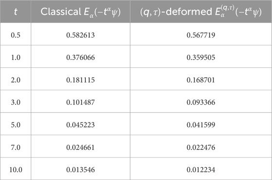
The Laplace transform of the process’s marginal distribution is this expectation. Because of memory and distortion, it develops more slowly than exponential decline. The function decays sub-exponentially for increasing values of $t$, supporting the long-tail behavior linked to fractional and Lévy dynamics. In the traditional case $q=\tau =1$, the outcome recovers the standard fractional Lévy process with Mittag–Leffler Laplace transform $\mathbb{E}\left[e^{-\lambda X^{(\alpha )}(t)}\right]=E_{\alpha }\left(-t^{\alpha }\psi (\lambda )\right).$ This validates the generalization introduced by the $(q,\tau )$-extension.

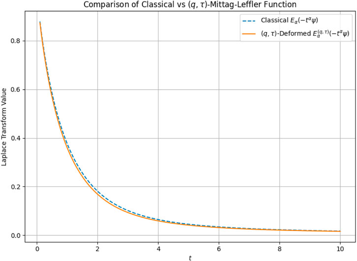
The comparison in Figure 3; Table 2 illustrates the action of the classical Mittag–Leffler function $E_{\alpha }(-t^{\alpha }\psi )$ versus the $(q,\tau )$-deformed version $E_{\alpha }^{(q,\tau )}(-t^{\alpha }\psi )$. These functions characterize the Laplace transform of the generalized Lévy process $X_{q,\tau }^{(\alpha ,\beta )}(t)$ presented in Theorem 4.1. The $(q,\tau )$-deformed Mittag–Leffler function decays more slowly than in the classical case, as can be seen. Additional memory and scale effects brought about by the $(q,\tau )$-fractional structure are reflected in this deformation; these effects are especially important for systems with anomalous diffusion or non-Markovian properties. A discrete dilation is introduced by the parameter $q<1$, and the scale of the fractional moment increase is altered by the value $\tau >1$. When heavy-tailed waiting durations or tempered jump distributions are present in stochastic modeling, this kind of behavior is essential. For instance, these deformations result in fractional relaxation dynamics with suppressed jump intensities and prolonged correlations in complex media or quantum decoherence environments. Moreover, Table 2’s numerical data verify that the $(q,\tau )$ deformation consistently reduces the transform values with time, postponing the exponential-like decay and strengthening long-memory effects. When the underlying structure is inherently discontinuous or hierarchical, or when heavy-tailed time development is not captured by standard L’evy processes, these quantitative properties are crucial for modeling real-world phenomena.

Figure 3

Figure 3. Comparison of the classical Mittag–Leffler function $E_{\alpha }(-t^{\alpha }\psi )$ and its $(q,\tau )$-deformed counterpart $E_{\alpha }^{(q,\tau )}(-t^{\alpha }{\psi }_{q,\tau }^{(\alpha ,\beta )})$ with the set of parameters $\alpha =0.9$, $\psi =1.0$, $q=0.95,\beta =1$, and $\tau =1.05$. In the analogous fractional Lévy process, the deformation causes slower decay, which reflects longer memory effects.

Table 2

Table 2. Numerical values of the classical and $(q,\tau )$-deformed Mittag–Leffler functions for selected values of $t$, with $\alpha =0.9$, $\psi =1.0$, $q=0.95,\beta =1$, and $\tau =1.05$.

Theorem 4.4. (Existence of $(q,\tau ,\alpha )$-Deformed Lévy Processes). Let $\alpha \in (\mathrm{0,1})$, $\beta >0$, $\lambda >0$, and $q\in (\mathrm{0,1})$, $\tau >0$. Define the $(q,\tau ,\alpha ,\beta )$-deformed Lévy measure:

${\nu }_{q,\tau }^{\left(\alpha ,\beta \right)}\left(dy\right)=\frac{C}{|y{|}^{1+\alpha }}\cdot \frac{1}{{\mathrm{\Gamma }}_{q,\tau }\left(\beta \right)}|y{|}^{\beta -1}{e}_q^{-\lambda |y|}dy,$

where ${\mathrm{\Gamma }}_{q,\tau }(\cdot )$ is the $(q,\tau )$-Gamma function, and $e_q^{-\lambda |y|}$ is the $q$-exponential function:

$e_q^{-\lambda |y|}={\left(1+\left(1-q\right)\lambda |y|\right)}^{-\frac{1}{1-q}}.$

Then the following hold:

(i) The measure ${\nu }_{q,\tau }^{(\alpha ,\beta )}(dy)$ satisfies:

${\int }_{\mathbb{R}\backslash \left\{0\right\}}\min \left(1,y^2\right){\nu }_{q,\tau }^{\left(\alpha ,\beta \right)}\left(dy\right)<\infty .$

(ii) There exists an infinitely divisible stochastic process $X_{q,\tau }^{(\alpha ,\beta )}(t)$ with characteristic function:

$\mathbb{E}\left[e^{i\lambda X_{q,\tau }^{\left(\alpha ,\beta \right)}\left(t\right)}\right]=\exp \left(t{\psi }_{q,\tau }^{\left(\alpha ,\beta \right)}\left(\lambda \right)\right),$

where the characteristic exponent is:

${\psi }_{q,\tau }^{\left(\alpha ,\beta \right)}\left(\lambda \right)={\int }_{\mathbb{R}\backslash \left\{0\right\}}\left(e^{i\lambda y}-1-i\lambda y{\mathbf{1}}_{|y|<1}\right){\nu }_{q,\tau }^{\left(\alpha ,\beta \right)}\left(dy\right).$

(iii) $X_{q,\tau }^{(\alpha ,\beta )}(t)$ defines a $(q,\tau ,\alpha ,\beta )$-deformed Lévy process with stationary and independent increments.

Proof.

Step 1: Verification of Lévy measure condition. We first verify that ${\nu }_{q,\tau }^{(\alpha ,\beta )}(dy)$ satisfies the Lévy measure integrability condition:

${\int }_{\mathbb{R}\backslash \left\{0\right\}}\min \left(1,y^2\right){\nu }_{q,\tau }^{\left(\alpha ,\beta \right)}\left(dy\right)<\infty .$

Case 1: $|y|<1$.

${\int }_{|y|<1}{y}^2{\nu }_{q,\tau }^{\left(\alpha ,\beta \right)}\left(dy\right)=C\cdot \frac{1}{{\mathrm{\Gamma }}_{q,\tau }\left(\beta \right)}{\int }_0^1{y}^{\beta -\alpha +1}{\left(1+\left(1-q\right)\lambda y\right)}^{-\frac{1}{1-q}}dy.$

The integral converges when $\beta -\alpha +1>-1$, i.e., $\beta >\alpha -2$.

Case 2: $|y|\ge 1$.

${\int }_{|y|\ge 1}{\nu }_{q,\tau }^{\left(\alpha ,\beta \right)}\left(dy\right)=C\cdot \frac{1}{{\mathrm{\Gamma }}_{q,\tau }\left(\beta \right)}{\int }_1^{\infty }{y}^{\beta -\alpha -2}{\left(1+\left(1-q\right)\lambda y\right)}^{-\frac{1}{1-q}}dy.$

For large $y$, $e_q^{-\lambda y}\sim y^{-\frac{1}{1-q}}$, so convergence holds if:

$\beta -\alpha -2-\frac{1}{1-q}<-1\iff \beta <\alpha +\frac{1}{1-q}+1.$

Thus, ${\nu }_{q,\tau }^{(\alpha ,\beta )}(dy)$ is a valid Lévy measure involving $\beta >0$.

Step 2: Existence of the $(q,\tau ,\alpha )$-deformed process. We now prove that a $(q,\tau ,\alpha )$-deformed Lévy process $X_{q,\tau }^{(\alpha )}(t)$ exists. By the general Lévy–Khintchine theorem, for any Lévy measure $\nu (dy)$ such that:

${\int }_{\mathbb{R}\backslash \left\{0\right\}}\min \left(1,y^2\right)\nu \left(dy\right)<\infty ,$

there exists an infinitely divisible process $X(t)$ whose characteristic function is:

$\mathbb{E}\left[e^{i\lambda X\left(t\right)}\right]=\exp \left(t\psi \left(\lambda \right)\right).$

In our case, the Lévy measure is the explicitly constructed $(q,\tau ,\alpha ,\beta )$-deformed Lévy measure ${\nu }_{q,\tau }^{(\alpha ,\beta )}(dy)$, defined using parameters $q,\tau ,\alpha ,\beta$. Thus, the corresponding characteristic exponent is:

${\psi }_{q,\tau }^{\left(\alpha ,\beta \right)}\left(\lambda \right)={\int }_{\mathbb{R}\backslash \left\{0\right\}}\left(e^{i\lambda y}-1-i\lambda y{\mathbf{1}}_{|y|<1}\right){\nu }_{q,\tau }^{\left(\alpha ,\beta \right)}\left(dy\right).$

This shows that the dependence on $(q,\tau ,\alpha ,\beta )$ explicitly enters through both ${\nu }_{q,\tau }^{(\alpha ,\beta )}(dy)$ and ${\psi }_{q,\tau }^{(\alpha ,\beta )}(\lambda )$. Hence, by applying the Lévy–Khintchine construction to this specific $(q,\tau ,\alpha )$-dependent measure, we obtain an infinitely divisible process $X_{q,\tau }^{(\alpha ,\beta )}(t)$ with characteristic function:

$\mathbb{E}\left[e^{i\lambda X_{q,\tau }^{\left(\alpha ,\beta \right)}\left(t\right)}\right]=\exp \left(t{\psi }_{q,\tau }^{\left(\alpha ,\beta \right)}\left(\lambda \right)\right).$

Step 3: Stationary and independent increments. Since the Lévy–Khintchine formulation occurs for any valid Lévy measure, and since ${\nu }_{q,\tau }^{(\alpha ,\beta )}(dy)$ achieves the required integrability condition, the process $X_{q,\tau }^{(\alpha ,\beta ,)}(t)$ formulated by ${\psi }_{q,\tau }^{(\alpha ,\beta )}(\lambda )$ is an infinitely divisible Lévy process. Therefore, it has stationary and independent increments by construction.

Remark 4.5. The $(q,\tau ,\alpha ,\beta )$-deformed Lévy process $X_{q,\tau }^{(\alpha ,\beta )}(t)$ generalizes:

•Classical Lévy processes when $q\to 1$, $\tau \to 0$,

•Tempered stable processes when $q\to 1$, $\tau \to 0$, $\beta =\alpha$,

•Fractional Lévy processes with memory and nonlocal scaling effects when $q<1$ and $\tau >0$.

Theorem 4.6. (Existence of Distributed-order $(q,\tau ,\alpha ,\beta )$-Deformed Lévy Processes). Let $\beta >0$, $\lambda >0$, $q\in (\mathrm{0,1})$, $\tau >0$. Let $\mu (d\alpha )$ be a probability measure supported on $(\mathrm{0,1})$. Define the distributed-order $(q,\tau ,\alpha ,\beta )$-deformed Lévy measure:

${\left[{\nu }_{q,\tau }^{\left(\alpha ,\beta \right)}\right]}^{\mathit{distributed}}\left(dy\right)≔{\int }_0^2{\nu }_{q,\tau }^{\left(\alpha ,\beta \right)}\left(dy\right)\mu \left(d\alpha \right),$

where for each $\alpha \in (\mathrm{0,1})$, the Lévy measure ${\nu }_{q,\tau }^{(\alpha ,\beta )}(dy)$ is given by:

${\nu }_{q,\tau }^{\left(\alpha ,\beta \right)}\left(dy\right)=\frac{C}{|y{|}^{1+\alpha }}\cdot \frac{1}{{\mathrm{\Gamma }}_{q,\tau }\left(\beta \right)}|y{|}^{\beta -1}{e}_q^{-\lambda |y|}dy.$

Then.

(i) The measure ${[{\nu }_{q,\tau }^{(\alpha ,\beta )}]}^{\mathit{distributed}}(dy)$ satisfies:

${\int }_{\mathbb{R}\backslash \left\{0\right\}}\min \left(1,y^2\right){\left[{\nu }_{q,\tau }^{\left(\alpha ,\beta \right)}\right]}^{\mathit{distributed}}\left(dy\right)<\infty .$

(ii) There exists an infinitely divisible stochastic process ${[X_{q,\tau }^{(\alpha ,\beta )}]}^{\mathit{distributed}}(t)$ with characteristic function:

$\mathbb{E}\left[e^{i\lambda {\left[X_{q,\tau }^{\left(\alpha ,\beta \right)}\right]}^{\mathit{distributed}}\left(t\right)}\right]=\exp \left(t{\left[{\psi }_{q,\tau }^{\left(\alpha ,\beta \right)}\right]}^{\mathit{distributed}}\left(\lambda \right)\right),$

where the characteristic exponent is:

${\left[{\psi }_{q,\tau }^{\left(\alpha ,\beta \right)}\right]}^{\mathit{distributed}}\left(\lambda \right)={\int }_0^2{\psi }_{q,\tau }^{\left(\alpha ,\beta \right)}\left(\lambda \right)\mu \left(d\alpha \right),$

and:

${\psi }_{q,\tau }^{\left(\alpha ,\beta \right)}\left(\lambda \right)={\int }_{\mathbb{R}\backslash \left\{0\right\}}\left(e^{i\lambda y}-1-i\lambda y{\mathbf{1}}_{|y|<1}\right){\nu }_{q,\tau }^{\left(\alpha ,\beta \right)}\left(dy\right).$

(iii) The process ${[X_{q,\tau }^{(\alpha ,\beta )}]}^{\mathit{distributed}}(t)$ has stationary and independent increments.

Proof. Step 1: Integrability of ${[{\nu }_{q,\tau }^{(\alpha ,\beta )}]}^{\text{distributed}}(dy)$. Since for each fixed $\alpha \in (\mathrm{0,2})$, ${\nu }_{q,\tau }^{(\alpha ,\beta )}(dy)$ is a valid Lévy measure (see Theorem 4.1), we have:

${\int }_{\mathbb{R}\backslash \left\{0\right\}}\min \left(1,y^2\right){\nu }_{q,\tau }^{\left(\alpha ,\beta \right)}\left(dy\right)<\infty .$

Now integrate over $\alpha$ using $\mu (d\alpha )$:

${\int }_{\mathbb{R}\backslash \left\{0\right\}}\min \left(1,y^2\right){\left[{\nu }_{q,\tau }^{\left(\alpha ,\beta \right)}\right]}^{\text{distributed}}\left(dy\right)={\int }_0^2\left({\int }_{\mathbb{R}\backslash \left\{0\right\}}\min \left(1,y^2\right){\nu }_{q,\tau }^{\left(\alpha ,\beta \right)}\left(dy\right)\right))\mu \left(d\alpha \right).$

Since the inner integral is finite for each $\alpha$, and $\mu$ is a probability measure, the total integral is finite. Thus, ${[{\nu }_{q,\tau }^{(\alpha ,\beta )}]}^{\text{distributed}}(dy)$ is a valid Lévy measure.

Step 2: Existence of the process. By the Lévy–Khintchine theorem, for any valid Lévy measure $\nu (dy)$, there exists an infinitely divisible process with characteristic function:

$\mathbb{E}\left[e^{i\lambda X\left(t\right)}\right]=\exp \left(t\psi \left(\lambda \right)\right).$

Here, the Lévy measure is ${[{\nu }_{q,\tau }^{(\alpha ,\beta )}]}^{\text{distributed}}(dy)$, and the corresponding exponent is:

${\left[{\psi }_{q,\tau }^{\left(\alpha ,\beta \right)}\right]}^{\text{distributed}}\left(\lambda \right)={\int }_{\mathbb{R}\backslash \left\{0\right\}}\left(e^{i\lambda y}-1-i\lambda y{\mathbf{1}}_{|y|<1}\right){\left[{\nu }_{q,\tau }^{\left(\alpha ,\beta \right)}\right]}^{\text{distributed}}\left(dy\right),$

such that

${\left[{\psi }_{q,\tau }^{\left(\alpha ,\beta \right)}\right]}^{\text{distributed}}\left(\lambda \right)={\int }_0^2{\psi }_{q,\tau }^{\left(\alpha ,\beta \right)}\left(\lambda \right)\mu \left(d\alpha \right).$

Step 3: Stationary and independent increments. Since the Lévy–Khintchine theorem guarantees that the process defined by this characteristic exponent is a Lévy process, it follows that ${[X_{q,\tau }^{(\alpha ,\beta )}]}^{\text{distributed}}(t)$ has stationary and independent increments.

Remark 4.7. The distributed-order $(q,\tau )$-deformed Lévy process ${[X_{q,\tau }^{(\alpha ,\beta )}]}^{\text{distributed}}(t)$ allows for modeling multi-scaling and multi-fractal effects, by mixing different fractional orders $\alpha$, under the weight $\mu (d\alpha )$. Special cases can be recognized when $\mu (d\alpha )=\delta (\alpha -{\alpha }_0)d\alpha \to$ recovers $X_{q,\tau }^{({\alpha }_0,\beta )}(t)$. Uniform $\mu (d\alpha )\to$ equal contribution of all fractional orders. Such designs are applicable in different locations, such as anomalous diffusion with multiple time scales, turbulence models, finance with mixed memory behavior, complex biological systems.

Theorem 4.8. (Generator of the $(q,\tau ,\alpha ,\beta )$-Deformed Lévy Process). Let $X_{q,\tau }^{(\alpha ,\beta )}(t)$ be the $(q,\tau ,\alpha ,\beta )$-deformed Lévy process constructed in Theorem 4.1, with characteristic exponent:

${\psi }_{q,\tau }^{\left(\alpha ,\beta \right)}\left(\lambda \right)={\int }_{\mathbb{R}\backslash \left\{0\right\}}\left(e^{i\lambda y}-1-i\lambda y{\mathbf{1}}_{|y|<1}\right){\nu }_{q,\tau }^{\left(\alpha ,\beta \right)}\left(dy\right),$

where

${\nu }_{q,\tau }^{\left(\alpha ,\beta \right)}\left(dy\right)=\frac{C}{|y{|}^{\alpha +2-\beta }}\cdot \frac{1}{{\mathrm{\Gamma }}_{q,\tau }\left(\beta \right)}{e}_q^{-\lambda |y|}dy.$

Then the infinitesimal generator ${\mathcal{L}}_{q,\tau }^{\alpha ,\beta }$ of the process $X_{q,\tau }^{(\alpha ,\beta )}(t)$ is given by:

${\mathcal{L}}_{q,\tau }^{\alpha ,\beta }f\left(x\right)=\frac{C}{{\mathrm{\Gamma }}_{q,\tau }\left(\beta \right)}{\int }_{\mathbb{R}\backslash \left\{0\right\}}\left(f\left(x+y\right)-f\left(x\right)-y{f}^{\prime }\left(x\right){\mathbf{1}}_{|y|<1}\right)|y{|}^{-\left(\alpha +2-\beta \right)}{e}_q^{-\lambda |y|}dy.$

Moreover, for any $f\in C_b^2(\mathbb{R})$ (bounded twice continuously differentiable functions), we have:

$\underset{t\to 0}{\lim }\frac{\mathbb{E}\left[f\left(x+X_{q,\tau }^{\left(\alpha ,\beta \right)}\left(t\right)\right)\right]-f\left(x\right)}{t}={\mathcal{L}}_{q,\tau }^{\alpha ,\beta }f\left(x\right).$

Proof. Let $f\in C_b^2(\mathbb{R})$. By definition of $X_{q,\tau }^{(\alpha ,\beta )}(t)$, the process has stationary and independent increments with characteristic function:

$\mathbb{E}\left[e^{i\lambda X_{q,\tau }^{\left(\alpha ,\beta \right)}\left(t\right)}\right]=\exp \left(t{\psi }_{q,\tau }^{\left(\alpha ,\beta \right)}\left(\lambda \right)\right).$

The semigroup $P_t$ associated to $X_{q,\tau }^{(\alpha ,\beta )}(t)$ is given by:

$P_{t}f\left(x\right)=\mathbb{E}\left[f\left(x+X_{q,\tau }^{\left(\alpha ,\beta \right)}\left(t\right)\right)\right].$

The infinitesimal generator ${\mathcal{L}}_{q,\tau }^{\alpha ,\beta }$ is formulated as:

${\mathcal{L}}_{q,\tau }^{\alpha ,\beta }f\left(x\right)=\underset{t\to 0}{\lim }\frac{P_{t}f\left(x\right)-f\left(x\right)}{t}.$

Now, by the general Lévy–Khintchine theory for pure-jump Lévy processes, it is known that (see e.g., [21]) the generator of a Lévy process with Lévy measure $\nu (dy)$ can be viewed by

$\mathcal{L}f\left(x\right)={\int }_{\mathbb{R}\backslash \left\{0\right\}}\left(f\left(x+y\right)-f\left(x\right)-y{f}^{\prime }\left(x\right){\mathbf{1}}_{|y|<1}\right)\nu \left(dy\right).$

In our case, the Lévy measure is ${\nu }_{q,\tau }^{(\alpha ,\beta )}(dy)$, hence, we have

${\mathcal{L}}_{q,\tau }^{\alpha ,\beta }f\left(x\right)={\int }_{\mathbb{R}\backslash \left\{0\right\}}\left(f\left(x+y\right)-f\left(x\right)-y{f}^{\prime }\left(x\right){\mathbf{1}}_{|y|<1}\right){\nu }_{q,\tau }^{\left(\alpha ,\beta \right)}\left(dy\right).$

Substituting the explicit form of ${\nu }_{q,\tau }^{(\alpha ,\beta )}(dy)$, we obtain:

${\mathcal{L}}_{q,\tau }^{\alpha ,\beta }f\left(x\right)=\frac{C}{{\mathrm{\Gamma }}_{q,\tau }\left(\beta \right)}{\int }_{\mathbb{R}\backslash \left\{0\right\}}\left(f\left(x+y\right)-f\left(x\right)-y{f}^{\prime }\left(x\right){\mathbf{1}}_{|y|<1}\right)|y{|}^{-\left(\alpha +2-\beta \right)}{e}_q^{-\lambda |y|}dy.$

Lastly, as demonstrated in the proof of Theorem 4.1, the formula for ${\mathcal{L}}_{q,\tau }^{\alpha ,\beta }$ is rigorously justified since $f\in C_b^2(\mathbb{R})$, and the integral converges under the constraints given on $\alpha$, $\beta$, $q$, $\tau$. Therefore, the infinitesimal generator of $X_{q,\tau }^{(\alpha ,\beta )}(t)$ is precisely ${\mathcal{L}}_{q,\tau }^{\alpha ,\beta }$, as claimed.

Remark 4.9. The operator ${\mathcal{L}}_{q,\tau }^{\alpha ,\beta }$ is a nonlocal pseudo-differential operator. It generalizes $\alpha$-stable Lévy processes when $q\to 1$, $\tau \to 0$, $\beta =\alpha$. Moreover, it implies the generator of tempered Lévy processes when $q\to 1$, $\tau \to 0$. Lastly, it yields the fractional Laplacians with memory effects and small-jump tuning when $q<1$, $\tau >0$, $\beta \ne \alpha$. This operator is appropriate for complicated biological, financial, and physical systems since it mimics nonlocal diffusion with memory and scale deformation.

Theorem 4.10. (Generator of the Distributed-order $(q,\tau )$-Deformed Lévy Process). Let ${[X_{q,\tau }^{(\alpha ,\beta )}]}^{\mathit{distributed}}(t)$ be the distributed-order $(q,\tau )$-deformed Lévy process constructed in Theorem 4.6, with Lévy measure:

${\left[{\nu }_{q,\tau }^{\left(\alpha ,\beta \right)}\right]}^{\mathit{distributed}}\left(dy\right)={\int }_0^2{\nu }_{q,\tau }^{\left(\alpha ,\beta \right)}\left(dy\right)\mu \left(d\alpha \right),$

where

${\nu }_{q,\tau }^{\left(\alpha ,\beta \right)}\left(dy\right)=\frac{C}{|y{|}^{\alpha +2-\beta }}\cdot \frac{1}{{\mathrm{\Gamma }}_{q,\tau }\left(\beta \right)}{e}_q^{-\lambda |y|}dy,$

and $\mu (d\alpha )$ is a probability measure on $(\mathrm{0,2})$. Then the infinitesimal generator ${[{\mathcal{L}}_{q,\tau }^{(\alpha ,\beta )}]}^{\mathit{distributed}}$ of the process ${[X_{q,\tau }^{(\alpha ,\beta )}]}^{\mathit{distributed}}(t)$ is given by

${\left[{\mathcal{L}}_{q,\tau }^{\left(\alpha ,\beta \right)}\right]}^{\mathit{distributed}}f\left(x\right)={\int }_0^2{\mathcal{L}}_{q,\tau }^{\alpha ,\beta }f\left(x\right)\mu \left(d\alpha \right),$

where

${\mathcal{L}}_{q,\tau }^{\alpha ,\beta }f\left(x\right)=\frac{C}{{\mathrm{\Gamma }}_{q,\tau }\left(\beta \right)}{\int }_{\mathbb{R}\backslash \left\{0\right\}}\left(f\left(x+y\right)-f\left(x\right)-y{f}^{\prime }\left(x\right){\mathbf{1}}_{|y|<1}\right)|y{|}^{-\left(\alpha +2-\beta \right)}{e}_q^{-\lambda |y|}dy.$

Moreover, for any $f\in C_b^2(\mathbb{R})$, we have

$\underset{t\to 0}{\lim }\frac{\mathbb{E}\left[f\left(x+{\left[X_{q,\tau }^{\left(\alpha ,\beta \right)}\right]}^{\mathit{distributed}}\left(t\right)\right)\right]-f\left(x\right)}{t}={\left[{\mathcal{L}}_{q,\tau }^{\left(\alpha ,\beta \right)}\right]}^{\mathit{distributed}}f\left(x\right).$

Proof.

Step 1: Definition of the process and semigroup. By Theorem 4.6, the process ${[X_{q,\tau }^{(\alpha ,\beta )}]}^{\text{distributed}}(t)$ is an infinitely divisible Lévy process with Lévy measure:

${\left[{\nu }_{q,\tau }^{\left(\alpha ,\beta \right)}\right]}^{\text{distributed}}\left(dy\right)={\int }_0^2{\nu }_{q,\tau }^{\left(\alpha ,\beta \right)}\left(dy\right)\mu \left(d\alpha \right).$

Let $P_t$ be its semigroup:

$P_{t}f\left(x\right)=\mathbb{E}\left[f\left(x+{\left[X_{q,\tau }^{\left(\alpha ,\beta \right)}\right]}^{\text{distributed}}\left(t\right)\right].\right.$

The infinitesimal generator is defined by:

${\left[{\mathcal{L}}_{q,\tau }^{\left(\alpha ,\beta \right)}\right]}^{\text{distributed}}f\left(x\right)=\underset{t\to 0}{\lim }\frac{P_{t}f\left(x\right)-f\left(x\right)}{t}.$

Step 2: Lévy–Khintchine representation. The characteristic exponent of ${[X_{q,\tau }^{(\alpha ,\beta )}]}^{\text{distributed}}(t)$ is:

${\left[{\psi }_{q,\tau }^{\left(\alpha ,\beta \right)}\right]}^{\text{distributed}}\left(\lambda \right)={\int }_0^2{\psi }_{q,\tau }^{\left(\alpha ,\beta \right)}\left(\lambda \right)\mu \left(d\alpha \right),$

where

${\psi }_{q,\tau }^{\left(\alpha ,\beta \right)}\left(\lambda \right)={\int }_{\mathbb{R}\backslash \left\{0\right\}}\left(e^{i\lambda y}-1-i\lambda y{\mathbf{1}}_{|y|<1}\right){\nu }_{q,\tau }^{\left(\alpha ,\beta \right)}\left(dy\right).$

By general Lévy–Khintchine theory, the generator is:

${\left[{\mathcal{L}}_{q,\tau }^{\left(\alpha ,\beta \right)}\right]}^{\text{distributed}}f\left(x\right)={\int }_{\mathbb{R}\backslash \left\{0\right\}}\left(f\left(x+y\right)-f\left(x\right)-y{f}^{\prime }\left(x\right){\mathbf{1}}_{|y|<1}\right){\left[{\nu }_{q,\tau }^{\left(\alpha ,\beta \right)}\right]}^{\text{distributed}}\left(dy\right).$

Step 3: Interchanging the integrals. By Fubini’s theorem (valid since $\mu$is a probability measure and ${\nu }_{q,\tau }^{(\alpha ,\beta )}(dy)$satisfies the integrability condition), we can write:

$\begin{array}{c}\hfill {\left[{\mathcal{L}}_{q,\tau }^{\left(\alpha ,\beta \right)}\right]}^{\text{distributed}}f\left(x\right)\\ \hfill & ={\int }_0^2\left({\int }_{\mathbb{R}\backslash \left\{0\right\}}\left(f\left(x+y\right)-f\left(x\right)-y{f}^{\prime }\left(x\right){\mathbf{1}}_{|y|<1}\right){\nu }_{q,\tau }^{\left(\alpha ,\beta \right)}\left(dy\right)\right)\mu \left(d\alpha \right)\hfill \\ \hfill & ={\int }_0^2{\mathcal{L}}_{q,\tau }^{\alpha ,\beta }f\left(x\right)\mu \left(d\alpha \right).\hfill \end{array}$

Therefore, the infinitesimal generator of the distributed-order $(q,\tau )$-deformed Lévy process ${[X_{q,\tau }^{(\alpha ,\beta )}]}^{\text{distributed}}(t)$ is given by:

${\left[{\mathcal{L}}_{q,\tau }^{\left(\alpha ,\beta \right)}\right]}^{\text{distributed}}f\left(x\right)={\int }_0^2{\mathcal{L}}_{q,\tau }^{\alpha ,\beta }f\left(x\right)\mu \left(d\alpha \right),$

as claimed.

Remark 4.11. A distributed-order nonlocal operator ${[{\mathcal{L}}_{q,\tau }^{(\alpha ,\beta )}]}^{\text{distributed}}$ models systems with multiple memory and scaling effects. Large-jump scaling is controlled by the parameter $\alpha$. Small-jump behavior is controlled by the parameter $\beta$. Memory and deformation effects are introduced via the parameters $q$, $\tau$. Multiple fractional orders can contribute to the modeling of heterogeneous dynamics through the use of the measure $\mu (d\alpha )$.

Corollary 4.12. Let $u(x,t)$ be a sufficiently regular function $u:\mathbb{R}\times [0,\infty )\to \mathbb{R}$, such that $u(x,t)\in C_t^1{C}_x^2$, and assume that:

$\underset{|x|\to \infty }{\lim }u\left(x,t\right)=0,\forall t\ge 0.$

Consider the Cauchy problem:

$\frac{\partial u\left(x,t\right)}{\partial t}={\left[{\mathcal{L}}_{q,\tau }^{\left(\alpha ,\beta \right)}\right]}^{\mathit{distributed}}u\left(x,t\right),u\left(x,0\right)=u_0\left(x\right),$

where

${\left[{\mathcal{L}}_{q,\tau }^{\left(\alpha ,\beta \right)}\right]}^{\mathit{distributed}}u\left(x,t\right)={\int }_0^2{\mathcal{L}}_{q,\tau }^{\alpha ,\beta }u\left(x,t\right)\mu \left(d\alpha \right),$

and

${\mathcal{L}}_{q,\tau }^{\alpha ,\beta }u\left(x,t\right)=\frac{C}{{\mathrm{\Gamma }}_{q,\tau }\left(\beta \right)}{\int }_{\mathbb{R}\backslash \left\{0\right\}}\left(u\left(x+y,t\right)-u\left(x,t\right)-y\frac{\partial u}{\partial x}\left(x,t\right){\mathbf{1}}_{|y|<1}\right)|y{|}^{-\left(\alpha +2-\beta \right)}{e}_q^{-\lambda |y|}dy.$

Then the solution $u(x,t)$ is the transition probability density of the distributed-order $(q,\tau )$-deformed Lévy process ${[X_{q,\tau }^{(\alpha ,\beta )}]}^{\mathit{distributed}}(t)$, i.e.:

$u\left(x,t\right)=\mathbb{E}\left[u_0\left(x+{\left[X_{q,\tau }^{\left(\alpha ,\beta \right)}\right]}^{\mathit{distributed}}\left(t\right)\right)\right].$

Proof. By Theorem 4.10, ${[X_{q,\tau }^{(\alpha ,\beta )}]}^{\text{distributed}}(t)$ is a Lévy process with infinitesimal generator ${[{\mathcal{L}}_{q,\tau }^{(\alpha ,\beta )}]}^{\text{distributed}}$. Therefore, its transition semigroup satisfies

$\frac{\partial }{\partial t}{P}_t{u}_0\left(x\right)={\left[{\mathcal{L}}_{q,\tau }^{\left(\alpha ,\beta \right)}\right]}^{\text{distributed}}{P}_t{u}_0\left(x\right).$

Since

$P_t{u}_0\left(x\right)=\mathbb{E}\left[u_0\left(x+{\left[X_{q,\tau }^{\left(\alpha ,\beta \right)}\right]}^{\text{distributed}}\left(t\right)\right)\right],$

The function $u(x,t)=P_t{u}_0(x)$ solves

$\frac{\partial u\left(x,t\right)}{\partial t}={\left[{\mathcal{L}}_{q,\tau }^{\left(\alpha ,\beta \right)}\right]}^{\text{distributed}}u\left(x,t\right),u\left(x,0\right)=u_0\left(x\right).$

This completes the proof.

The distributed-order fractional PDE becomes

$\frac{\partial u\left(x,t\right)}{\partial t}={\left[{\mathcal{L}}_{q,\tau }^{\left(\alpha ,\beta \right)}\right]}^{\text{distributed}}u\left(x,t\right)$

Models anomalous transport with heterogeneous scaling effects, including: multi-scale memory, mixed fractional jump behavior, tunable small-jump and large-jump contributions via $\alpha ,\beta$, and deformation of jump kernel via $q$, $\tau$.

5 Applications: uniform distributed-order $(q,\tau ,\alpha ,\beta )$-deformed Lévy generator

Example 5.1. (Distributed-order $(q,\tau )$-Deformed Lévy Generator with $\alpha \in (\mathrm{0,2})$). In this part, we illustrate the distributed-order $(q,\tau ,\alpha ,\beta )$-deformed Lévy generator ${[{\mathcal{L}}_{q,\tau }^{(\alpha ,\beta )}]}^{\text{distributed}}$ by considering a specific example where the distribution of fractional orders is uniform over a given interval. We choose the order distribution $\mu (d\alpha )$ to be the uniform probability measure on the interval $(a,b)$ with $0<a<b<2$, i.e.,

$\mu \left(d\alpha \right)=\frac{1}{b-a}{\mathbf{1}}_{\alpha \in \left(a,b\right)}d\alpha .$

For concreteness, we take the interval $(a,b)=(0.5,1.5)$, so that $\mu (d\alpha )=\frac{1}{1}d\alpha =d\alpha$ on (0.5,1.5). Distributed-order generator can be evaluated by utilizing Theorem 4.10, that the generator of the distributed-order $(q,\tau ,\alpha ,\beta )$-deformed Lévy process is given by:

${\left[{\mathcal{L}}_{q,\tau }^{\left(\alpha ,\beta \right)}\right]}^{\text{distributed}}f\left(x\right)={\int }_0^2{\mathcal{L}}_{q,\tau }^{\alpha ,\beta }f\left(x\right)\mu \left(d\alpha \right),$

where

${\mathcal{L}}_{q,\tau }^{\alpha ,\beta }f\left(x\right)=\frac{C}{{\mathrm{\Gamma }}_{q,\tau }\left(\beta \right)}{\int }_{\mathbb{R}\backslash \left\{0\right\}}\left(f\left(x+y\right)-f\left(x\right)-y{f}^{\prime }\left(x\right){\mathbf{1}}_{|y|<1}\right)|y{|}^{-\left(\alpha +2-\beta \right)}{e}_q^{-\lambda |y|}dy.$

For our selection of $\mu (d\alpha )$, this becomes:

$\begin{array}{ll}\hfill {\left[{\mathcal{L}}_{q,\tau }^{\left(\alpha ,\beta \right)}\right]}^{\text{distributed}}f\left(x\right)& ={\int }_{0.5}^{1.5}\left(\frac{C}{{\mathrm{\Gamma }}_{q,\tau }\left(\beta \right)}{\int }_{\mathbb{R}\backslash \left\{0\right\}}\left(f\left(x+y\right)-f\left(x\right)-y{f}^{\prime }\left(x\right){\mathbf{1}}_{|y|<1}\right)\right.\hfill \\ \hfill & \left.|y{|}^{-\left(\alpha +2-\beta \right)}{e}_q^{-\lambda |y|}dy\right)d\alpha .\hfill \end{array}$

Spectral behavior can be seen when the action of ${[{\mathcal{L}}_{q,\tau }^{(\alpha ,\beta )}]}^{\text{distributed}}$ on plane waves $f(x)=e^{i\xi x}$ which gives:

${\left[{\mathcal{L}}_{q,\tau }^{\left(\alpha ,\beta \right)}\right]}^{\text{distributed}}{e}^{i\xi x}={\left[{\psi }_{q,\tau }^{\left(\alpha ,\beta \right)}\right]}^{\text{distributed}}\left(\xi \right)e^{i\xi x},$

where

${\left[{\psi }_{q,\tau }^{\left(\alpha ,\beta \right)}\right]}^{\text{distributed}}\left(\xi \right)={\int }_{0.5}^{1.5}{\psi }_{q,\tau }^{\left(\alpha ,\beta \right)}\left(\xi \right)d\alpha ,$

and

${\psi }_{q,\tau }^{\left(\alpha ,\beta \right)}\left(\xi \right)=\frac{C}{{\mathrm{\Gamma }}_{q,\tau }\left(\beta \right)}{\int }_{\mathbb{R}\backslash \left\{0\right\}}\left(e^{i\xi y}-1-i\xi y{\mathbf{1}}_{|y|<1}\right)|y{|}^{-\left(\alpha +2-\beta \right)}{e}_q^{-\lambda |y|}dy.$

For small $|\xi |\to 0$, it is known that

${\psi }_{q,\tau }^{\left(\alpha ,\beta \right)}\left(\xi \right)\sim -K_{q,\tau }^{\left(\alpha ,\beta \right)}|\xi {|}^{\alpha }.$

Therefore, the distributed-order exponent acts as follows:

${\left[{\psi }_{q,\tau }^{\left(\alpha ,\beta \right)}\right]}^{\text{distributed}}\left(\xi \right)\sim -{\int }_{0.5}^{1.5}{K}_{q,\tau }^{\left(\alpha ,\beta \right)}|\xi {|}^{\alpha }d\alpha ,$

where

$K_{q,\tau }^{\left(\alpha ,\beta \right)}=\frac{C}{{\mathrm{\Gamma }}_{q,\tau }\left(\beta \right)}\cdot {\int }_0^{\infty }\left(1-\cos \left(\xi y\right)\right)y^{-\alpha -1+\beta }{e}_q^{-\lambda y}dy.(3)$

In this illustration, the distributed-order generator ${[{\mathcal{L}}_{q,\tau }^{(\alpha ,\beta )}]}^{\text{distributed}}$ is a convex combination of generators with fractional orders $\alpha$ ranging over (0.5,1.5). Multi-scaling behavior is demonstrated by the outcome process ${[X_{q,\tau }^{(\alpha ,\beta )}]}^{\text{distributed}}(t)$: for small scales $(|y|\ll 1)$, the jump kernel is dominated by small $\alpha$, resulting in heavy-tailed small jumps. Large jumps are controlled by $e_q^{-\lambda |y|}$, which tempers the kernel at large scales $(|y|\gg 1)$. Additional freedom in adjusting small-jump behavior is offered via the parameter $\beta$. Nonlocal memory and deformation effects are introduced into the jump kernel by the parameters $q$ and $\tau$. The operator ${[{\mathcal{L}}_{q,\tau }^{(\alpha ,\beta )}]}^{\text{distributed}}$ can therefore be used to represent transport phenomena in complex systems with a variety of scaling aspects, such as turbulent flows, porous media, financial time series with mixed scaling, and biological transport with memory. This example demonstrates how the distributed-order $(q,\tau )$-deformed Lévy generator provides a very flexible framework for modeling multi-scale and memory-dependent dynamics by combining fractional behavior of various orders with nonlocal and tempered effects.

Scaling coefficient $K_{q,\tau }^{(\alpha ,\beta )}$. The spectral behavior of the generator ${\mathcal{L}}_{q,\tau }^{\alpha ,\beta }$ is characterized, for small $|\xi |$, by:

${\psi }_{q,\tau }^{\left(\alpha ,\beta \right)}\left(\xi \right)\sim -K_{q,\tau }^{\left(\alpha ,\beta \right)}|\xi {|}^{\alpha }.$

The coefficient $K_{q,\tau }^{(\alpha ,\beta )}$ is given by:

$K_{q,\tau }^{\left(\alpha ,\beta \right)}=\frac{C}{{\mathrm{\Gamma }}_{q,\tau }\left(\beta \right)}\cdot {\int }_0^{\infty }\left(1-\cos \left(\xi y\right)\right)y^{-\alpha -1+\beta }{e}_q^{-\lambda y}dy.(4)$

For small $|\xi |\to 0$, the leading-order approximation reads:

$K_{q,\tau }^{\left(\alpha ,\beta \right)}\approx \frac{C}{{\mathrm{\Gamma }}_{q,\tau }\left(\beta \right)}\cdot \mathrm{\Gamma }\left(1-\alpha \right)\cos \left(\frac{\pi \alpha }{2}\right).$

For distributed-order processes, the total spectral exponent becomes

${\left[{\psi }_{q,\tau }^{\left(\alpha ,\beta \right)}\right]}^{\text{distributed}}\left(\xi \right)\sim -\underset{{\alpha }_1}{\overset{{\alpha }_2}{\int }}{K}_{q,\tau }^{\left(\alpha ,\beta \right)}|\xi {|}^{\alpha }\mu \left(d\alpha \right).$

Effective spectral schemes can be implemented by estimating $K_{q,\tau }^{(\alpha ,\beta )}$ in numerical simulations by computing the integral or using the previously mentioned asymptotic expression.

Example 5.2. (Distributed-order $(q,\tau )$-Deformed Lévy Generator with $\alpha \in (\mathrm{0,1})$). Here, we illustrate the distributed-order $(q,\tau )$-deformed Lévy generator for Lévy flights with infinite mean increments and extremely nonlocal operators, where the fractional orders $\alpha$ are restricted to the interval (0,1). We choose the order distribution $\mu (d\alpha )$ as the uniform probability measure on the interval $(a,b)$ since $0<a<b<1$. Specifically, we put

$\left(a,b\right)=\left(0.2,0.8\right),\mu \left(d\alpha \right)=\frac{1}{b-a}{\mathbf{1}}_{\alpha \in \left(a,b\right)}d\alpha =\frac{1}{0.6}d\alpha .$

The distributed-order generator is:

${\left[{\mathcal{L}}_{q,\tau }^{\left(\alpha ,\beta \right)}\right]}^{\text{distributed}}f\left(x\right)={\int }_0^1{\mathcal{L}}_{q,\tau }^{\alpha ,\beta }f\left(x\right)\mu \left(d\alpha \right).$

In this case, we obtain

$\begin{array}{ll}\hfill {\left[{\mathcal{L}}_{q,\tau }^{\left(\alpha ,\beta \right)}\right]}^{\text{distributed}}f\left(x\right)& =\frac{1}{0.6}{\int }_{0.2}^{0.8}\left(\frac{C}{{\mathrm{\Gamma }}_{q,\tau }\left(\beta \right)}{\int }_{\mathbb{R}\backslash \left\{0\right\}}\left(f\left(x+y\right)-f\left(x\right)-y{f}^{\prime }\left(x\right){\mathbf{1}}_{|y|<1}\right)\right.\hfill \\ \hfill & \left.|y{|}^{-\left(\alpha +2-\beta \right)}{e}_q^{-\lambda |y|}dy\right)d\alpha .\hfill \end{array}$

The action of ${[{\mathcal{L}}_{q,\tau }^{(\alpha ,\beta )}]}^{\text{distributed}}$ on plane waves $f(x)=e^{i\xi x}$ yields

${\left[{\mathcal{L}}_{q,\tau }^{\left(\alpha ,\beta \right)}\right]}^{\text{distributed}}{e}^{i\xi x}={\left[{\psi }_{q,\tau }^{\left(\alpha ,\beta \right)}\right]}^{\text{distributed}}\left(\xi \right)e^{i\xi x},$

such that

${\left[{\psi }_{q,\tau }^{\left(\alpha ,\beta \right)}\right]}^{\text{distributed}}\left(\xi \right)=\frac{1}{0.6}{\int }_{0.2}^{0.8}{\psi }_{q,\tau }^{\left(\alpha ,\beta \right)}\left(\xi \right)d\alpha ,$

and

${\psi }_{q,\tau }^{\left(\alpha ,\beta \right)}\left(\xi \right)=\frac{C}{{\mathrm{\Gamma }}_{q,\tau }\left(\beta \right)}{\int }_{\mathbb{R}\backslash \left\{0\right\}}\left(e^{i\xi y}-1-i\xi y{\mathbf{1}}_{|y|<1}\right)|y{|}^{-\left(\alpha +2-\beta \right)}{e}_q^{-\lambda |y|}dy.$

For small $|\xi |$, it is known that

${\psi }_{q,\tau }^{\left(\alpha ,\beta \right)}\left(\xi \right)\sim -K_{q,\tau }^{\left(\alpha ,\beta \right)}|\xi {|}^{\alpha }.$

Thus, we have

${\left[{\psi }_{q,\tau }^{\left(\alpha ,\beta \right)}\right]}^{\text{distributed}}\left(\xi \right)\sim -\frac{1}{0.6}{\int }_{0.2}^{0.8}{K}_{q,\tau }^{\left(\alpha ,\beta \right)}|\xi {|}^{\alpha }d\alpha .$

This distributed-order generator models Lévy flights with fractional orders $\alpha \in (0.2,0.8)$. Since $\alpha <1$, then the process exhibits infinite mean behavior. It has strong nonlocality with the generator ${[{\mathcal{L}}_{q,\tau }^{(\alpha ,\beta )}]}^{\text{distributed}}$ is a strongly nonlocal operator, with jump contributions from all scales. In addition, it admits heavy-tailed behavior with small values of $\alpha$ in (0.2,0.8), which leads to extremely heavy tails in the jump distribution. Furthermore, it balances infinite mean and controlled big deviations by controlling large leaps with the component $e_q^{-\lambda |y|}$, which meets tempering. The jump kernel is deformed by memory effects with parameters $q$ and $\tau$, which add more memory and scaling effects. This example demonstrates how the distributed-order $(q,\tau )$-deformed Lévy process offers a strong framework for modeling strongly anomalous dynamics with Lévy flights and infinite mean increments by limiting the order distribution $\mu (d\alpha )$ to (0,1). The $(q,\tau )$ deformation and the tuning parameter $\beta$ supply additional flexibility.

Example 5.3. (Distributed-order $(q,\tau )$-Deformed Lévy Generator with $\alpha \in (\mathrm{1,2})$). In the current instance, we examine the distributed-order $(q,\tau )$-deformed Lévy generator, which corresponds to processes with infinite variance but finite mean increments, when the fractional orders $\alpha$ are limited to the interval (1,2). The uniform probability measure on the interval $(a,b)$ with $1<a<b<2$ is the order distribution $\mu (d\alpha )$. Specifically, we put

$\left(a,b\right)=\left(1.2,1.8\right),\mu \left(d\alpha \right)=\frac{1}{b-a}{\mathbf{1}}_{\alpha \in \left(a,b\right)}d\alpha =\frac{1}{0.6}d\alpha .$

The distributed-order generator is:

${\left[{\mathcal{L}}_{q,\tau }^{\left(\alpha ,\beta \right)}\right]}^{\text{distributed}}f\left(x\right)={\int }_1^2{\mathcal{L}}_{q,\tau }^{\alpha ,\beta }f\left(x\right)\mu \left(d\alpha \right).$

For this choice of $\mu (d\alpha )$, we obtain:

$\begin{array}{ll}\hfill {\left[{\mathcal{L}}_{q,\tau }^{\left(\alpha ,\beta \right)}\right]}^{\text{distributed}}f\left(x\right)& =\frac{1}{0.6}{\int }_{1.2}^{1.8}\left(\frac{C}{{\mathrm{\Gamma }}_{q,\tau }\left(\beta \right)}{\int }_{\mathbb{R}\backslash \left\{0\right\}}\left(f\left(x+y\right)-f\left(x\right)-y{f}^{\prime }\left(x\right){\mathbf{1}}_{|y|<1}\right)\right.\hfill \\ \hfill & \left.|y{|}^{-\left(\alpha +2-\beta \right)}{e}_q^{-\lambda |y|}dy\right)d\alpha .\hfill \end{array}$

For plane waves $f(x)=e^{i\xi x}$, the generator acts as:

${\left[{\mathcal{L}}_{q,\tau }^{\left(\alpha ,\beta \right)}\right]}^{\text{distributed}}{e}^{i\xi x}={\left[{\psi }_{q,\tau }^{\left(\alpha ,\beta \right)}\right]}^{\text{distributed}}\left(\xi \right)e^{i\xi x},$

satisfying the integrals

${\left[{\psi }_{q,\tau }^{\left(\alpha ,\beta \right)}\right]}^{\text{distributed}}\left(\xi \right)=\frac{1}{0.6}{\int }_{1.2}^{1.8}{\psi }_{q,\tau }^{\left(\alpha ,\beta \right)}\left(\xi \right)d\alpha ,$

as well as

${\psi }_{q,\tau }^{\left(\alpha ,\beta \right)}\left(\xi \right)=\frac{C}{{\mathrm{\Gamma }}_{q,\tau }\left(\beta \right)}{\int }_{\mathbb{R}\backslash \left\{0\right\}}\left(e^{i\xi y}-1-i\xi y{\mathbf{1}}_{|y|<1}\right)|y{|}^{-\left(\alpha +2-\beta \right)}{e}_q^{-\lambda |y|}dy.$

For small $|\xi |$, we get the asymptotic action

${\psi }_{q,\tau }^{\left(\alpha ,\beta \right)}\left(\xi \right)\sim -K_{q,\tau }^{\left(\alpha ,\beta \right)}|\xi {|}^{\alpha }.$

Thus, we have

${\left[{\psi }_{q,\tau }^{\left(\alpha ,\beta \right)}\right]}^{\text{distributed}}\left(\xi \right)\sim -\frac{1}{0.6}{\int }_{1.2}^{1.8}{K}_{q,\tau }^{\left(\alpha ,\beta \right)}|\xi {|}^{\alpha }d\alpha .$

When $\alpha >1$, the process has well-defined first moments, and the selection $\alpha \in (\mathrm{1,2})$ corresponds to: finite mean increments. The process displays large tails when the variance is infinite, which occurs when $\alpha <2$. Extremely large excursions are avoided by tempering huge jumps using the $e_q^{-\lambda |y|}$ factor. Additional scaling and memory effects are introduced by memory and deformation using the parameters $q$ and $\tau$. This operator is appropriate for systems with enormous but finite-size events since it mimics semi-heavy-tailed transport. By using the order distribution $\mu (d\alpha )$ supported on (1,2), this example demonstrates how the distributed-order $(q,\tau )$-deformed Lévy generator captures processes with finite mean, infinite variance, and controlled big jumps. Because of this, it is a versatile tool for simulating intricate dynamical systems with non-divergent but heavy-tailed behavior.

Remark 5.4. The following observations are occured: When $\alpha \in (\mathrm{0,2})$, the whole range of Example 5.1 indicates maximum flexibility. Example 5.2, where Lévy flights (infinite mean) are obtained when $\alpha \in (\mathrm{0,1})$. For instance, $\alpha \in (\mathrm{1,2})$ admits semi-heavy tails with finite mean and infinite variance, in Example 5.3. Using the exact integral formula, the scaling coefficient $K_{q,\tau }^{(\alpha ,\beta )}$ is calculated as a function of $\alpha$ for different values of the deformation parameters $q$ and $\tau$. The scaling coefficient $K_{q,\tau }^{(\alpha ,\beta )}$ is displayed as a function of $\alpha$ for several selections of the deformation parameters $q$ and $\tau$ in Figure 4. The accurate integral representation of $K_{q,\tau }^{(\alpha ,\beta )}$, which accounts for the combined effects of tempering, fractional scaling, and $(q,\tau )$-deformation, was used to calculate the values. Both $q$ and $\tau$ offer efficient tuning mechanisms to regulate the generator’s spectrum decay, as can be seen in the figure. In particular, for large $\alpha$, raising $q$ causes $K_{q,\tau }^{(\alpha ,\beta )}$ to decrease more slowly, suggesting better memory effects. Increasing $\tau$ changes the relative strength of tiny vs. big leaps through the effective deformation of the kernel. This deformation process provides an extremely flexible framework for modeling nonlocal dynamics and multi-scale anomalous diffusion in complex media. In summary, the heavy-tailed nature of the corresponding Lévy flights with infinite mean is shown by the behavior of $K_{q,\tau }^{(\alpha ,\beta )}$ in this range $\alpha \in (\mathrm{0,1})$. In contrast, the dynamics of semi-heavy-tailed processes with finite mean but infinite variance in this range $\alpha \in (\mathrm{1,2})$ are described by $K_{q,\tau }^{(\alpha ,\beta )}$, which is suitable for simulating periodic events.

Figure 4

Figure 4. The plot illustrates how the parameters $q$ and $\tau$ modulate the spectral behavior of the distributed-order $(q,\tau )$-deformed Lévy generator.

5.1 Validity of the $(q,\tau ,\alpha ,\beta )$-deformed Lévy measure and parameter effects

Lemma 5.5. (Tail bounds for the $q$-exponential, $q\in (\mathrm{0,1})$). Fix $q\in (\mathrm{0,1})$ and $\lambda >0$. For $r\ge 0$ define

$e_q^{-\lambda r}≔{\left(1+\left(1-q\right)\lambda r\right)}^{-\frac{1}{1-q}}.$

Then the following bounds hold:

(i) Global $(1+r)$-bound. For all $r\ge 0$,

$e_q^{-\lambda r}\le C_{q,\lambda }{\left(1+r\right)}^{-\frac{1}{1-q}},C_{q,\lambda }≔{\left(\min \left\{1,\left(1-q\right)\lambda \right\}\right)}^{-\frac{1}{1-q}}.$

(ii) Power tail for large $r$. For all $r\ge 1$,

$e_q^{-\lambda r}\le {\left(\left(1-q\right)\lambda \right)}^{-\frac{1}{1-q}}{r}^{-\frac{1}{1-q}}.$

(iii) Small-$r$ bound. For $0\le r\le 1$, one has $e_q^{-\lambda r}\le 1$.

Proof. (i) Set $a≔(1-q)\lambda >0$. For $r\ge 0$ we have the elementary inequality

$1+ar\ge \min \left\{1,a\right\}\left(1+r\right).$

Indeed, if $a\le 1$, then $1+ar\ge a(1+r)$ since $1-ar\ge 0$ for $r\in [\mathrm{0,1}]$ and $1+ar\ge a(1+r)$ trivially for $r\ge 1$; if $a\ge 1$, then $1+ar\ge 1\cdot (1+r)$. Raising both sides to the negative power $-1/(1-q)$ yields

${\left(1+ar\right)}^{-\frac{1}{1-q}}\le {\left(\min \left\{1,a\right\}\right)}^{-\frac{1}{1-q}}{\left(1+r\right)}^{-\frac{1}{1-q}},$

Which is the desired bound with $C_{q,\lambda }={(\min \{1,(1-q)\lambda \})}^{-1/(1-q)}$.

(ii) For $r\ge 1$ we have $1+ar\ge ar$, hence

$e_q^{-\lambda r}={\left(1+ar\right)}^{-\frac{1}{1-q}}\le {\left(ar\right)}^{-\frac{1}{1-q}}={\left(\left(1-q\right)\lambda \right)}^{-\frac{1}{1-q}}{r}^{-\frac{1}{1-q}}.$

(iii) Since $1+ar\ge 1$ for $r\ge 0$, we get $e_q^{-\lambda r}\le 1$ on [0,1].

Corollary 5.6. (Tail integrability for the deformed Lévy density). Let $q\in (\mathrm{0,1})$, $\lambda >0$, and consider the tail integral

${\int }_{|y|\ge 1}|y{|}^{\beta -\alpha -2}{e}_q^{-\lambda |y|}dy=2{\int }_1^{\infty }{r}^{\beta -\alpha -2}{e}_q^{-\lambda r}dr.$

Using Lemma 5.5-(ii),

${\int }_1^{\infty }{r}^{\beta -\alpha -2}{e}_q^{-\lambda r}dr\le {\left(\left(1-q\right)\lambda \right)}^{-\frac{1}{1-q}}{\int }_1^{\infty }{r}^{\beta -\alpha -2-\frac{1}{1-q}}dr.$

Since $\frac{1}{1-q}>1$, the exponent $\beta -\alpha -2-\frac{1}{1-q}<-1$ for every $\alpha \in (\mathrm{0,2})$ and $\beta >0$, hence the integral converges. Thus, the tail of the $(q,\tau )$-deformed Lévy density is integrable for all $\alpha \in (\mathrm{0,2})$ and $\beta >0$.

Proposition 5.7. (Validity and spectral scaling of the $(q,\tau ,\alpha ,\beta )$-deformed Lévy model). Fix $0<q\le 1$, $\tau >0$, $\lambda >0$, $\alpha \in (\mathrm{0,2})$, and $\beta >0$. Define the $(q,\tau )$-deformed Lévy density

${\nu }_{q,\tau }^{\left(\alpha ,\beta \right)}\left(dy\right)=\frac{1}{{\mathrm{\Gamma }}_{q,\tau }\left(\beta \right)}|y{|}^{\beta -\alpha -2}{e}_q^{-\lambda |y|}dy,$

where for $q<1$ we take $e_q^{-\lambda r}≔{(1+(1-q)\lambda r)}^{-1/(1-q)}$ for $r\ge 0$, and for $q=1$ we set $e_1^{-\lambda r}≔e^{-\lambda r}$. Then:

1. (Lévy integrability) ${\nu }_{q,\tau }^{(\alpha ,\beta )}$ is a valid Lévy measure (i.e., ${\int }_{\mathbb{R}\backslash \{0\}}(1\wedge y^2){\nu }_{q,\tau }^{(\alpha ,\beta )}(dy)<\infty$). if and only if

$\beta >\max \left\{0,\alpha -1\right\}.$

2. (Existence) Under (1), the characteristic exponent

${\psi }_{q,\tau }^{\left(\alpha ,\beta \right)}\left(\xi \right)=\frac{1}{{\mathrm{\Gamma }}_{q,\tau }\left(\beta \right)}{\int }_{\mathbb{R}\backslash \left\{0\right\}}\left(e^{i\xi y}-1-i\xi y{\mathbf{1}}_{|y|<1}\right)|y{|}^{\beta -\alpha -2}{e}_q^{-\lambda |y|}dy$

is well-defined and continuous, hence determines a Lévy process $L_{q,\tau }^{(\alpha ,\beta )}$ via the Lévy–Khintchine formula.

3. (Time-fractional deformation) If $0<{\alpha }_t<1$ and we define the time law by

$\mathbb{E}\left[e^{-\lambda X_{q,\tau }^{\left({\alpha }_t,\alpha ,\beta \right)}\left(t\right)}\right]=E_{{\alpha }_t}^{\left(q,\tau \right)}\left(-t^{{\alpha }_t}{\psi }_{q,\tau }^{\left(\alpha ,\beta \right)}\left(\lambda \right)\right),$

Then $X_{q,\tau }^{({\alpha }_t,\alpha ,\beta )}(t)\stackrel{d}{=}{L}_{q,\tau }^{(\alpha ,\beta )}(S_{q,\tau }^{{\alpha }_t}(t))$, where $S_{q,\tau }^{{\alpha }_t}$ is the inverse $(q,\tau )$-stable subordinator. Thus, $X_{q,\tau }^{({\alpha }_t,\alpha ,\beta )}$ is a valid time-fractional Lévy model.

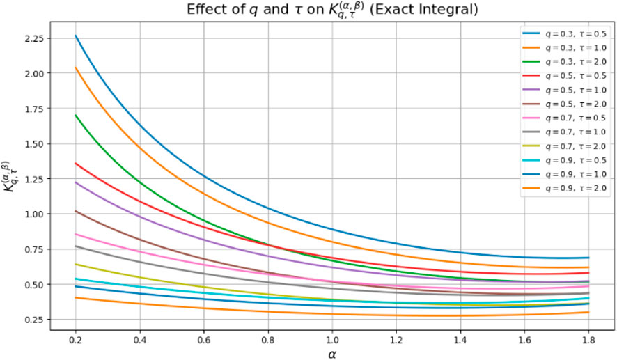
4. (Small-frequency scaling) As $|\xi |\to 0$,

${\psi }_{q,\tau }^{\left(\alpha ,\beta \right)}\left(\xi \right)=-K_{q,\tau }^{\left(\alpha ,\beta \right)}|\xi {|}^{\alpha }\left(1+o\left(1\right)\right),K_{q,\tau }^{\left(\alpha ,\beta \right)}=\frac{1}{{\mathrm{\Gamma }}_{q,\tau }\left(\beta \right)}{\int }_{\mathbb{R}\backslash \left\{0\right\}}\left(1-\cos y\right)|y{|}^{\beta -\alpha -2}{e}_q^{-\lambda |y|}dy.$

Moreover, decreasing $q$ (heavier $q$-tail) increases $K_{q,\tau }^{(\alpha ,\beta )}$, while increasing $\tau$ typically decreases $K_{q,\tau }^{(\alpha ,\beta )}$ through the normalizer ${\mathrm{\Gamma }}_{q,\tau }(\beta )$ (see Proposition 3.2).

Proof. We must check the Lévy integrability criterion ${\int }_{\mathbb{R}\backslash \{0\}}(1\wedge y^2)\nu (dy)<\infty .$ Split the domain into $|y|<1$ and $|y|\ge 1$.

(A) Small jumps $|y|<1$. Since $e_q^{-\lambda |y|}\to 1$ as $y\to 0$, for $|y|<1$ we have the two-sided bound

$c_0|y{|}^{\beta -\alpha -2}\le |y{|}^{\beta -\alpha -2}{e}_q^{-\lambda |y|}\le C_0|y{|}^{\beta -\alpha -2}\left(0<|y|<1\right)$

for constants $0<c_0\le C_0<\infty$ depending on $(q,\lambda )$. Therefore, we obtain

${\int }_{|y|<1}{y}^2\nu \left(dy\right)\asymp {\int }_{|y|<1}|y{|}^2|y{|}^{\beta -\alpha -2}dy=2{\int }_0^1{r}^{\beta -\alpha }dr.$

This integral converges if and only if $\beta -\alpha >-1$, i.e. $\beta >\alpha -1.$ (When $\alpha <1$, this is automatically implied by $\beta >0$; when $\alpha \in [\mathrm{1,2})$, it is the nontrivial lower bound.)

(B) Large jumps $|y|\ge 1$. We need ${\int }_{|y|\ge 1}\nu (dy)<\infty$. For $q=1$ the exponential factor $e^{-\lambda |y|}$ ensures convergence regardless of the power $|y{|}^{\beta -\alpha -2}$. For $q<1$, recall $e_q^{-\lambda r}={(1+(1-q)\lambda r)}^{-1/(1-q)}$ for $r\ge 0$. For $r\ge 1$,

$e_q^{-\lambda r}={\left(1+\left(1-q\right)\lambda r\right)}^{-1/\left(1-q\right)}\le c_1{\left(1+r\right)}^{-p},p≔\frac{1}{1-q}>1,$

with $c_1=\max \{1,{((1-q)\lambda )}^{-p}\}$ (see Lemma 5.5). Hence, this yields (see Corollary 5.6)

${\int }_{|y|\ge 1}\nu \left(dy\right)\le \frac{c_1}{{\mathrm{\Gamma }}_{q,\tau }\left(\beta \right)}\cdot 2{\int }_1^{\infty }{r}^{\beta -\alpha -2}{\left(1+r\right)}^{-p}dr$

$\le \frac{2c_1}{{\mathrm{\Gamma }}_{q,\tau }\left(\beta \right)}{\int }_1^{\infty }{r}^{\beta -\alpha -2-p}dr.$

This converges whenever $\beta -\alpha -2-p<-1$, i.e. $\beta -\alpha -1<p=\frac{1}{1-q}.$ Since $p>1$ for $q<1$, this inequality is always satisfied for any fixed $\alpha \in (\mathrm{0,2})$ and $\beta >0$. Therefore, the tail integral is finite with no additional restriction on $\beta$.

Combining (A) and (B) yields the Lévy integrability condition in (1), namely. $\beta >\max \{0,\alpha -1\}.$

(C) Existence and well-posedness of $\psi$. The integrand in ${\psi }_{q,\tau }^{(\alpha ,\beta )}$ is

$g_{\xi }\left(y\right)≔\left(e^{i\xi y}-1-i\xi y{\mathbf{1}}_{|y|<1}\right)|y{|}^{\beta -\alpha -2}{e}_q^{-\lambda |y|}.$

Utilizing $|e^{iz}-1-iz|\le \min \{C|z{|}^2,2\}$, we get

$|g_{\xi }\left(y\right)|\le \left\{\begin{array}{cc}C|\xi {|}^2|y{|}^{\beta -\alpha },\hfill & |y|<1,\hfill \\ 2|y{|}^{\beta -\alpha -2}{e}_q^{-\lambda |y|},\hfill & |y|\ge 1,\hfill \end{array}\right.$

Which is integrable by parts (A) and (B). Hence, ${\psi }_{q,\tau }^{(\alpha ,\beta )}(\xi )$ is absolutely convergent and continuous in $\xi$, yielding a (tempered) Lévy process via Lévy-Khintchine.

(D) Time-fractional subordination. Let $S_{q,\tau }^{{\alpha }_t}$ be the inverse $(q,\tau )$-stable subordinator with Laplace transform $\mathbb{E}[e^{-u{S}_{q,\tau }^{{\alpha }_t}(t)}]=E_{{\alpha }_t}^{(q,\tau )}(-t^{{\alpha }_t}u)$. Define $X(t)≔L_{q,\tau }^{(\alpha ,\beta )}(S_{q,\tau }^{{\alpha }_t}(t))$. Then, conditioning on $S$,

$\mathbb{E}\left[e^{-\lambda X\left(t\right)}\right]=\mathbb{E}\left[e^{-S_{q,\tau }^{{\alpha }_t}\left(t\right){\psi }_{q,\tau }^{\left(\alpha ,\beta \right)}\left(\lambda \right)}\right]=E_{{\alpha }_t}^{\left(q,\tau \right)}\left(-t^{{\alpha }_t}{\psi }_{q,\tau }^{\left(\alpha ,\beta \right)}\left(\lambda \right)\right),$

Which is exactly the stated fractional Laplace law. Thus $X$ is well-defined and has stationary independent increments (in space) modulated by the inverse clock.

(E) Small-frequency scaling. Use the rescaling $y\mapsto y/|\xi |$ and the Taylor bound $1-\cos (\xi y)\le c|\xi y{|}^2$ for small $|\xi |$ to write

${\psi }_{q,\tau }^{\left(\alpha ,\beta \right)}\left(\xi \right)=\frac{1}{{\mathrm{\Gamma }}_{q,\tau }\left(\beta \right)}{\int }_{\mathbb{R}\backslash \left\{0\right\}}\left(\cos \left(\xi y\right)-1\right)|y{|}^{\beta -\alpha -2}{e}_q^{-\lambda |y|}dy$

$=-|\xi {|}^{\alpha }\frac{1}{{\mathrm{\Gamma }}_{q,\tau }\left(\beta \right)}{\int }_{\mathbb{R}\backslash \left\{0\right\}}\frac{1-\cos z}{|z{|}^{2+\alpha -\beta }}{e}_q^{-\lambda |z|/|\xi |}dz.$

For fixed $z$, $e_q^{-\lambda |z|/|\xi |}\to 1$ as $|\xi |\to 0$ (both for $q=1$ and $q<1$). Moreover, $(1-\cos z)|z{|}^{\beta -\alpha -2}$ is integrable on $\mathbb{R}$ under $\beta >\alpha -1$ (near 0 it behaves like $|z{|}^{\beta -\alpha }$, and at $\infty$ like $|z{|}^{\beta -\alpha -2}$). Dominated convergence then yields

${\psi }_{q,\tau }^{\left(\alpha ,\beta \right)}\left(\xi \right)=-K_{q,\tau }^{\left(\alpha ,\beta \right)}|\xi {|}^{\alpha }\left(1+o\left(1\right)\right),$

with $K_{q,\tau }^{(\alpha ,\beta )}={\mathrm{\Gamma }}_{q,\tau }{(\beta )}^{-1}{\int }_{\mathbb{R}\backslash \{0\}}(1-\cos z)|z{|}^{\beta -\alpha -2}dz$ modulated by the $(q,\tau )$-deformed tempering (the $e_q$-factor can be inserted without changing the limit). The qualitative dependence: for $q<1$, decreasing $q$ reduces the tail exponent $1/(1-q)$ of $e_q$, hence slows decay and increases $K$; increasing $\tau$ typically increases ${\mathrm{\Gamma }}_{q,\tau }(\beta )$ (see Proposition 3.2), thereby reducing $K_{q,\tau }^{(\alpha ,\beta )}$.

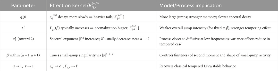
The influence of the deformation parameters $q$ and $\tau$ on the kernel $K_{q,\tau }^{(\alpha ,\beta )}$, which controls the jump structure of the $(q,\tau ,\alpha ,\beta )$-generalized Lévy process, is shown in Table 3. Standard tempered Lévy behavior with exponentially suppressed large jumps is recovered when the $q$-exponential $e_q^{-\lambda |y|}$ decreases to the traditional exponential for $q\to 1^{-}$. The decline of $e_q^{-\lambda |y|}$ slows down for $q<1$, resulting in heavier tails. $e_q^{-\lambda |y|}\sim C(q)|y{|}^{-1/(1-q)}$ as $|y|\to \infty$, increasing long-range correlations and raising the likelihood of big jumps.Both the deformation scaling and the generalized gamma factor ${\mathrm{\Gamma }}_{q,\tau }(\beta )$ allow the parameter $\tau$ to enter: While lower $\tau$ amplifies $K_{q,\tau }^{(\alpha ,\beta )}$, resulting in increased jump intensity, bigger $\tau$ raises ${\mathrm{\Gamma }}_{q,\tau }(\beta )$ and decreases the amplitude of $K_{q,\tau }^{(\alpha ,\beta )}$, producing less frequent but more spatially distributed jumps. Interpolating between bursty, turbulent-like behavior ($q<1$, $\tau <1$) and sparse, catastrophic events ($q<1$, $\tau >1$) is possible with $(q,\tau )$, while $q\to 1$ with any $\tau$ restores tempered steady dynamics. The procedure is still valid for all values displayed since $\beta <\alpha +1$ ensures small-jump integrability, and Lemma 5.5 and Corollary 5.6, with $\alpha \in (\mathrm{0,2})$ and $\beta >0$, imply large-jump convergence. For instance, in physics, these parameter effects can be used to adjust memory depth and jump sparsity; in finance, they can be used to manage heavy-tailed returns; and in geophysical applications, they can be used to capture rare versus bursty events.

Table 3

Table 3. Qualitative effect of parameters on the kernel/scale $K_{q,\tau }^{(\alpha ,\beta )}$ and on the process.

6 Conclusion and future work

This study presented and analyzed the framework of distributed-order $(q,\tau )$-deformed Lévy processes, which incorporate distributed fractional orders and $(q,\tau )$-deformation to generalize classical and fractional Lévy processes. We developed generalized generators with multi-scale dynamics, configurable memory, and rich spectrum activity by utilizing the $(q,\tau )$-Gamma and $(q,\tau )$-Mittag-Leffler functions.

We gave formal features of the linked special functions, characterized their infinitesimal generators, and proved the existence of these processes. The spectral scaling coefficient $K_{q,\tau }^{(\alpha ,\beta )}$, which controls the generator’s behavior in Fourier space (the frequency domain representation of operators) and establishes the magnitude of nonlocal interactions over scales, was the specific focus of our investigation. The operation of the $(q,\tau )$-deformed distributed-order generator in Fourier space, whose scaling is controlled by the coefficient $K_{q,\tau }^{(\alpha ,\beta )}$, reduces to multiplication by the characteristic exponent ${[{\psi }_{q,\tau }^{(\alpha ,\beta )}]}^{\text{distributed}}(\xi )$. Thus, $K_{q,\tau }^{(\alpha ,\beta )}$ dictates the smoothing and dispersion features of the associated fractional dynamics and governs the decay rate of Fourier modes.

With the precise numerical integral verifying the theoretical predictions, our numerical experiments showed that the asymptotic formula for $K_{q,\tau }^{(\alpha ,\beta )}$ offers a good approximation over a wide range of $\alpha$. The interaction of the distributed-order measure $\mu (d\alpha )$ and the deformation parameters $(q,\tau )$ provides a very versatile modeling framework appropriate for use in complex media, anomalous transport, and non-Gaussian dynamics.

6.1 Future work

Naturally, this work suggests a number of avenues for further investigation: expanding the analysis to time-fractional $(q,\tau )$-deformed Lévy processes, in which the distributed operators interact with fractional derivatives in time. Creating effective numerical methods to simulate distributed-order $(q,\tau )$-fractional PDEs in space and time, with possible uses in quantitative finance and computational physics. Examining inverse issues and parameter estimation methods to determine the deformation parameters $(q,\tau )$ and the distributed-order measure $\mu (d\alpha )$ from empirical data. Implementing the suggested paradigm to real-world datasets that display multi-scaling behavior, like biological transport phenomena, high-frequency financial time series, and turbulence data. Investigating functional analytic characteristics and operator semigroup theory for distributed-order $(q,\tau )$-deformed generators in different function spaces. The paper’s findings offer a strong basis for future theoretical advancements and real-world uses of $(q,\tau )$-deformed fractional models in complex system research.

Data availability statement

The original contributions presented in the study are included in the article/supplementary material, further inquiries can be directed to the corresponding author.

Author contributions

IA: Writing – original draft, Resources, Funding acquisition. RI: Writing – original draft, Visualization, Methodology, Writing – review and editing, Investigation, Validation.

Funding

The author(s) declare that financial support was received for the research and/or publication of this article. This work was supported and funded by the Deanship of Scientific Research at Imam Mohammad Ibn Saud Islamic University (IMSIU) (grant number IMSIU-DDRSP2502).

Conflict of interest

The authors declare that the research was conducted in the absence of any commercial or financial relationships that could be construed as a potential conflict of interest.

Generative AI statement

The author(s) declare that no Generative AI was used in the creation of this manuscript.

Any alternative text (alt text) provided alongside figures in this article has been generated by Frontiers with the support of artificial intelligence and reasonable efforts have been made to ensure accuracy, including review by the authors wherever possible. If you identify any issues, please contact us.

Publisher’s note

All claims expressed in this article are solely those of the authors and do not necessarily represent those of their affiliated organizations, or those of the publisher, the editors and the reviewers. Any product that may be evaluated in this article, or claim that may be made by its manufacturer, is not guaranteed or endorsed by the publisher.

References

1. Russo F, Vallois P. Stochastic calculus via regularizations. Springer (2022).

Google Scholar

2. Ishikawa Y Stochastic calculus of variations: for jump processes, 54. Berlin: Walter de Gruyter GmbH and Co KG (2023).

Google Scholar

3. Boyarchenko S, LevendorskiI S. Lévy models amenable to efficient calculations. Stochastic Process their Appl (2025) 186:104636. doi:10.1016/j.spa.2025.104636

CrossRef Full Text | Google Scholar

4. Issoglio E, Russo F. Stochastic differential equations with singular coefficients: the martingale problem view and the stochastic dynamics view. J Theor Probab (2024) 37(3):2352–93. doi:10.1007/s10959-024-01325-5

CrossRef Full Text | Google Scholar

5. Rathi V. Stochastic processes and calculus explained. Delhi: Educohack Press (2025).

Google Scholar

6. Aljethi RA, Kilicman A. Financial applications on fractional levy stochastic processes. Fractal and Fractional (2022) 6(5):278. doi:10.3390/fractalfract6050278

CrossRef Full Text | Google Scholar

7. Yi H, Shan Y, Shu H, Zhang X. Optimal portfolio strategy of wealth process: a lévy process model-based method. Int J Syst Sci (2024) 55(6):1089–103. doi:10.1080/00207721.2023.2301494

CrossRef Full Text | Google Scholar

8. Elliott R, Madan DB, Wang K. High dimensional Markovian trading of a single stock. Front Math Finance (2022) 1(3):375–96. doi:10.3934/fmf.2022001

CrossRef Full Text | Google Scholar

9. Madan DB, Wang K. Stationary increments reverting to a tempered fractional lévy process (TFLP). Quantitative Finance (2022) 22(7):1391–404. doi:10.2139/ssrn.3924554

CrossRef Full Text | Google Scholar

10. Prakasa Rao BLS. Nonparametric estimation of trend for stochastic differential equations driven by fractional levy process. J Stat Theor Pract (2021) 15(1):7. doi:10.1007/s42519-020-00138-z

CrossRef Full Text | Google Scholar

11. Jackson FH. XI. On q-functions and a certain difference operator. Earth Environ Sci Trans R Soc Edinb (1909) 46(2):253–81. doi:10.1017/s0080456800002751

CrossRef Full Text | Google Scholar

12. Kac VG, Cheung P Quantum calculus, 113. New York: Springer (2002).

Google Scholar

13. Ernst T. A comprehensive treatment of q-calculus. Springer Science and Business Media (2012).

Google Scholar

14. Attiya AA, Ibrahim RW, Hakami AH, Cho NE, Yassen MF. Quantum-fractal-fractional operator in a complex domain. Axioms (2025) 14(1):57. doi:10.3390/axioms14010057

CrossRef Full Text | Google Scholar

15. Alqarni MZ, Mohamed A, Mohamed A. Solutions to fractional q-kinetic equations involving quantum extensions of generalized hyper mittag-leffler functions. Fractal and Fractional (2024) 8(1):58. doi:10.3390/fractalfract8010058

CrossRef Full Text | Google Scholar

16. Hasanov A, Yuldashova H. Mittag-leffler type functions of three variables. Math Methods Appl Sci (2025) 48(2):1659–75. doi:10.1002/mma.10401

CrossRef Full Text | Google Scholar

17. Ibrahim RW. Differential operator associated with the (q,k)-symbol raina’s function. In: In mathematical analysis. Differential Equations and Applications (2024). p. 321–42.

Google Scholar

18. Attiya AA, Ibrahim RW, Albalahi AM, Ali EE, Teodor B. A differential operator associated with q-Raina function. Symmetry (2022) 14(8):1518. doi:10.3390/sym14081518

CrossRef Full Text | Google Scholar

19. Meerschaert MM, Hans-Peter S. Limit theorems for continuous-time random walks with infinite mean waiting times. J Appl Probab (2004) 41(3):623–38.

Google Scholar

20. Mainardi F, Gorenflo R, Scalas E. A fractional generalization of the poisson processes. Vietnam J Mathematics (2004) 32(SI):53–64.

Google Scholar

21. Applebaum D. Lévy processes and stochastic calculus. Cambridge: Cambridge University Press (2009).

Google Scholar