 Wu-Yue Pang1,2
 Li Lin1,3*
- 1Department of Finance, Business School, East China University of Science and Technology, Shanghai, China
- 2School of Information Science and Engineering, East China University of Science and Technology, Shanghai, China
- 3Risk-Center, ETH Zürich, Zürich, Switzerland
Understanding systemic risk in financial markets requires tools that capture both structural complexity and dynamic evolution. This study adopts a complex systems perspective to analyze the Chinese stock market through correlation-based state classification. Using multidimensional scaling and K-means clustering on rolling stock return correlations, we identify five distinct market states that reflect varying degrees of systemic co-movement and exhibit strong temporal persistence and local transition patterns. We find that transitions among these states encode meaningful information about market structural shifts and are closely linked to the emergence of crash conditions. Building on this insight, we construct an early warning model using decision trees trained on temporal features derived from market state transitions—including medium-term state distributions, directional change ratios, and short-term evolutionary paths. The model achieves high recall and precision across configurations, and supports real-time adaptability via projection-based state labeling. These results highlight the value of market state dynamics and their transitions as a basis for systemic risk monitoring and crash anticipation in complex financial systems.
1 Introduction
Financial markets are widely regarded as complex adaptive systems, in which the interactions among heterogeneous agents give rise to emergent phenomena such as volatility clustering, contagion, and crashes [1–4]. Capturing these dynamics requires moving beyond isolated asset-level indicators to examine the structure and evolution of market-wide interactions. In this context, correlation-based and network-theoretic representations have emerged as powerful tools for modeling systemic behavior. Early studies constructed networks from return correlation matrices to quantify collective dynamics and market fragility [5, 6], while more recent work has introduced higher-order interaction structures, including Granger-causality networks [7], speculative influence networks [8], portfolio overlap networks [9], and Ricci-curvature-based geometric approaches [10, 11]. These approaches collectively highlight the importance of modeling financial markets as evolving structures whose topological and temporal features govern their stability—serving, in effect, as emergent order parameters that summarize the global configuration of the system [12, 13]. In parallel, recent advances in econometric modeling have enriched this structural perspective through dynamic correlation and network connectivity analyses [14], contagion mechanism estimation [15], and cross-sectional uncertainty metrics [16], offering additional insights into the spatiotemporal propagation of systemic stress.
Building on these foundations, a growing body of research has demonstrated that financial markets can be decomposed into a small number of discrete market states, derived from clustering time-dependent correlation matrices [17–19]. These states are understood to reflect varying levels of market-wide coordination, with high-correlation regimes typically aligned with heightened systemic risk. Crucially, transitions between these states are not random but exhibit structured, often persistent patterns—indicative of path-dependent dynamics rooted in collective behavior and feedback effects [20, 21]. This suggests that financial instability is less a sudden shock than a gradual process, emerging from shifts in the system’s internal organization and the evolution of its interaction topology. Such state transitions are also closely related to latent patterns of risk contagion and inter-market connectivity, as highlighted in recent econometric models of dynamic transmission mechanisms and time-zone-adjusted VAR frameworks [15]. Moreover, advances in modeling cross-sectional uncertainty have shown promise in enhancing correlation-based classification methods, offering insights into the predictive structure of latent regimes [16]. These perspectives collectively underscore the need to treat state transitions not merely as clustering artifacts, but as meaningful structural shifts reflecting endogenous risk propagation.
Despite these advances, several important aspects remain underexplored in the existing literature. First, most studies are retrospective in nature—focusing on identifying and interpreting market states ex post—without translating these structural insights into forward-looking monitoring tools. Second, while emerging research suggests that market state transitions encode valuable early signals of systemic stress [22, 23], relatively few studies have formally integrated such temporal patterns into operational early warning systems. This issue is especially relevant in the context of emerging markets such as China, where distinctive market microstructures from developed market and investor behaviors complicate risk assessment. Existing models often lack structural interpretability and real-time adaptability, underscoring the need for monitoring frameworks that reflect the endogenous evolution of systemic fragility [24–26].
To address the aforementioned limitations, this paper proposes a structure-aware early warning framework that explicitly incorporates the temporal dynamics of market state transitions. Using the CSI 300 Index as a representative system, we first identify five distinct market states through a combination of correlation-based similarity measures, multidimensional scaling (MDS), and K-means clustering. These states correspond to different levels of systemic coupling and exhibit empirically stable transition patterns: transitions occur predominantly between adjacent states, while high-correlation regimes are disproportionately associated with historical crash periods.
Leveraging these insights, we develop a decision tree-based early warning model constructed from temporally structured features of market state dynamics. These include medium-term state distributions, directional transition ratios, and recent evolutionary motifs. The model demonstrates high recall and precision under cross-validation and remains robust when extended to new data via an efficient projection-based labeling mechanism. Crucially, unlike traditional indicators based on instantaneous correlation structure—such as the Absorption Ratio (AR) [6] and its extension ARR [27], eigenvalue-based early warning signals [20], or curvature-derived fragility measures [10, 11]—our framework emphasizes the predictive value of how structural regimes evolve over time. This transition-centric approach provides a dynamic lens on market fragility, enhancing the model’s interpretability and its potential for real-time monitoring in complex financial environments.
To the best of our understanding, few studies have systematically leveraged market state transitions—interpreted as emergent order-parameter dynamics within complex systems—to inform supervised early warning models, particularly in the context of emerging markets. This study seeks to bridge complex systems modeling with practical risk monitoring by operationalizing structurally grounded state transitions as interpretable signals for crash forecasting.
The remainder of the paper is organized as follows. Section 2.1 introduces the methodology for identifying correlation-driven market states and modeling their temporal transitions. Section 2.2 details the decision tree-based early warning model, including the design of interpretable state-informed features and projection-based labeling of new data. Section 3.2 presents empirical analysis of 15 years of CSI 300 data, covering market state classification, transition dynamics, and their link to crash periods. Section 4 evaluates the early warning model, focusing on feature configuration tuning, performance assessment, and interpretation of decision paths related to pre-crash signals. Section 5 concludes with key findings and implications for systemic risk monitoring and future research.
2 Methods
2.1 Market state classification and labeling
We conceptualize the financial market as a complex system, where its internal structure is reflected in the correlation patterns among individual stocks. A market state, in this context, is defined by the collective behavior of these correlations. To distinguish different states over time, we assess how the correlation structure evolves across different time windows, mainly following the approach proposed by Pharasi et al. [17, 19]. Specifically, we measure the similarity of correlation matrices computed over these windows, treating similar correlation patterns as indicators of the same underlying market state. To construct the correlation matrices, we begin with daily post-rights-adjusted prices of all stocks and assemble them into a data matrix. The logarithmic return of each stock
where
The average
where
By applying this transformation, we obtain a sequence of noise-suppressed correlation matrices
We now define a similarity measure (or distance) between two correlation matrices,
where the overline denotes the average over all matrix elements. These pairwise distances are then used as input for Multidimensional Scaling (MDS), which projects the matrices into a low-dimensional space while preserving their mutual distances within an acceptable tolerance. MDS aims to map each correlation matrix
where each entry
where
In this study, we select
We then apply
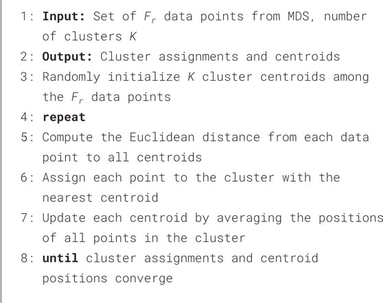
Algorithm 1.
To determine the optimal number of clusters
To determine the optimal number of clusters
where
While this formulation resembles the structure of the Akaike Information Criterion (AIC), it is not derived from a traditional likelihood framework. Rather, it draws on a probabilistic interpretation of K-means under isotropic statistical assumptions and inspired by the information-theoretic model selection principle of balancing model complexity and goodness-of-fit [29]. To avoid confusion, we refer to it as a pseudo-AIC, and provide a detailed justification of this formulation in Supplementary Appendix A. The value of pseudo-AIC balances model fit and complexity, penalizing models with a large number of clusters. We select the optimal number of clusters
In our analysis, we primarily consider cases where
2.2 Early warning model for market crash using machine learning methods
The first step in constructing the machine learning-based early warning model is to define the binary classification labels: market crash cases
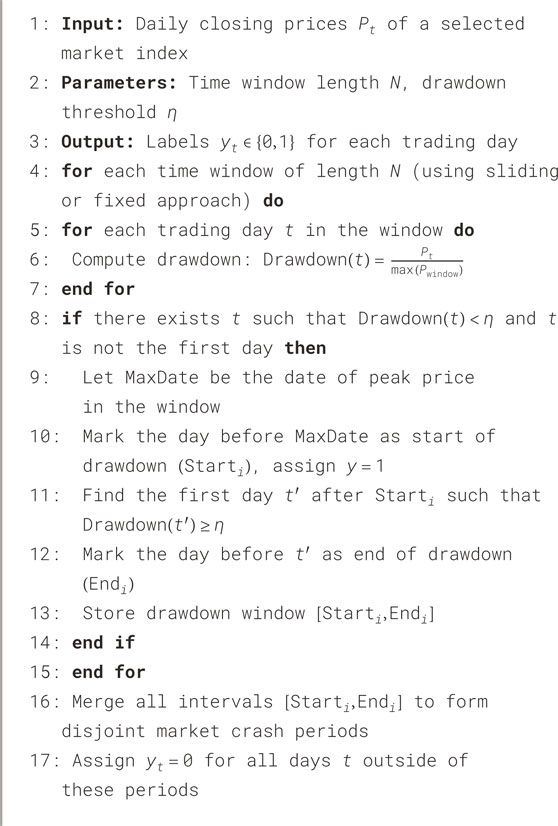
Algorithm 2. Labeling Market Crash Cases from Market Price Data.
In this paper, we employ the decision trees to construct the market crash early warning model. This modeling choice is motivated by several considerations. Decision trees are inherently simple yet highly interpretable, offering a clear hierarchical structure of decision rules that makes them particularly well-suited for applications requiring transparent reasoning. Second, they are relatively robust to overfitting, especially when the model complexity (e.g., tree depth) is properly controlled. Third, and most importantly in our context, decision trees are well-suited to scenarios with a limited number of input features. Since our early warning model is constructed based on market state transitions—resulting in a compact, semantically meaningful feature set—the ability of decision trees to perform reliable classification without requiring high-dimensional input is a critical advantage. These properties allow the model to maintain strong generalization performance while ensuring interpretability for financial analysts and policy researchers.
To enhance predictive performance, there are three types of features to be implemented to extract patterns associated with market state transitions in pre-crash dynamics:
This process yields
Although the state indices themselves are agnostic to specific economic meanings, empirical observations—both from our subsequent empirical results and related literature—suggest that transitions toward higher-indexed states tend to coincide with increased structural complexity or market disorder. Hence, a high value of
(3) Evolutionary Path of Market States in the Nearest
Each unique sequence of
These pattern-based features are particularly useful for capturing local dynamics, including sudden structural shifts, oscillatory behavior, or persistent regime patterns within stable/unstable conditions. By encoding the short-run evolutionary trajectory of market states, this feature set complements other indicators focused on medium- and long-term structural characteristics.
Given the asymmetric costs associated with classification outcomes in this context—where missing a true crash event (false negative) may result in significantly more severe consequences than issuing a false alarm (false positive)—the model selection process is designed to prioritize recall. Among models achieving the highest recall, further selection is made by jointly considering overall classification accuracy and minimizing the false positive rate (FPR), thereby ensuring both sensitivity and precision in practical application.
To address the issue of model adaptability over time, we further consider how to incorporate newly arriving data without compromising model consistency. A key challenge lies in assigning market state labels to new incoming time points. Re-clustering the entire dataset whenever new data becomes available is computationally expensive and introduces instability, particularly near cluster boundaries, where minor perturbations may lead to significant reassignments and undermine the validity of previously extracted features. Moreover, substantial updates in data may necessitate a recalibration of clustering hyper-parameters, including the optimal number of clusters and the noise suppression coefficient. To mitigate these issues, we propose the following procedure: compute the similarity (or distance) between the new data and the historical correlation matrices defined in Section 2.1, apply MDS algorithms to project the new observation into the same low-dimensional space, and subsequently assign its cluster label using a computationally efficient classifier (e.g., SVM) trained on the original MDS-embedded data.
3 The state transition behavior of the Chinese Stock Market
3.1 Data
This study utilizes the daily post-rights-adjusted prices of constituent stocks from the CSI 300 Index. The CSI 300, comprising 300 large-cap and highly liquid stocks from both the Shanghai and Shenzhen stock exchanges, represents approximately 60% of the total market capitalization of China’s A-share market. As such, it serves as a key indicator for tracking the overall performance of the Chinese stock market. Its constituents are typically industry-leading enterprises that are highly responsive to sectoral and macroeconomic developments. Fluctuations in their stock prices tend to promptly reflect market sentiment and investor expectations, making them particularly suitable for investigating market state transitions.
Focusing on CSI 300 constituents allows the study to capture systemic market dynamics using a representative sample set, balancing analytical validity with computational efficiency. For the empirical analysis, there are 285 stocks selected from the CSI 300 Index, covering a 15-year period from January 2010 to December 2024, corresponding to
3.2 Identification of market states
We compute the logarithmic returns of the daily post-adjusted closing prices for each stock and generate a sequence of 3,621 correlation matrices of dimension 285 using a sliding window approach, with the window length set to
Figure 1 presents the landscape of pseudo AIC-adjusted standard deviations across a grid of cluster counts (
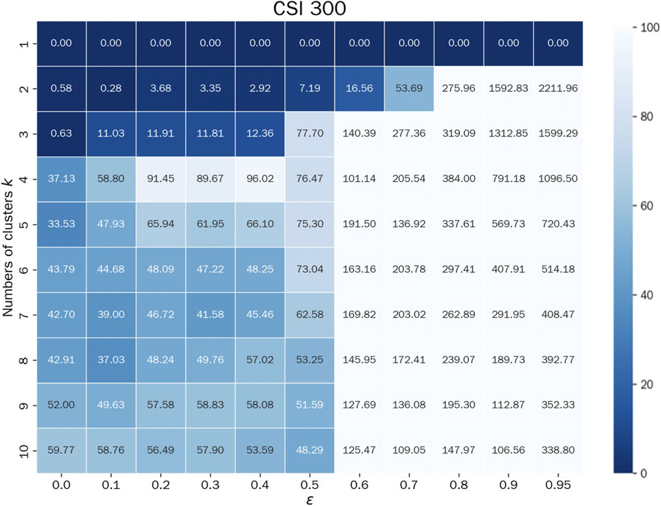
Figure 1. Stability landscape for clustering: Pseudo AIC-Adjusted standard deviation across
As discussed in Section 2.1, although configurations with
Figure 2a presents a two-dimensional projection of the clustering result onto the xz-plane, derived from the optimal three-dimensional embedding obtained via MDS. This projection facilitates intuitive visualization of the cluster separation in reduced dimensions. The full three-dimensional representation of the MDS result, as shown in Figure 2b, provides a more comprehensive view of the geometric structure underlying the correlation matrices. Together, these visualizations demonstrate that the five identified market states are well-separated in the embedded space, suggesting the presence of latent structural patterns in market behavior over time.
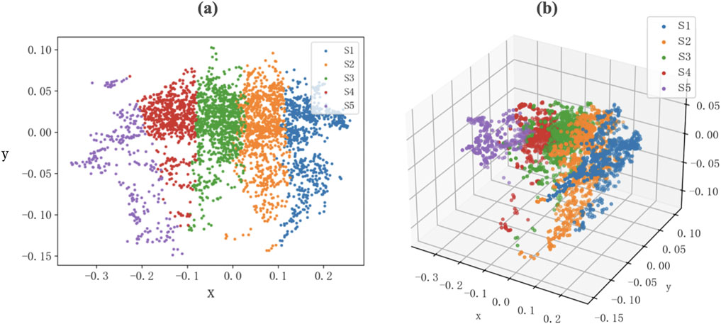
Figure 2. Multidimensional scaling (MDS) visualization of market state clustering.
Figure 3 presents example heatmaps of stock return correlation matrices for 285 constituent stocks, each selected from a representative trading day corresponding to one of the five identified market states under the configuration
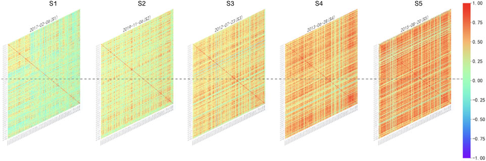
Figure 3. Representative correlation structures across market states.
To capture the temporal dynamics of market conditions, we examine the evolution of state occupancy probabilities over time. The color blocks in Figure 4 represent the relative frequency of each market state within semiannual windows. Specifically, the probability of a state in each window reflects the proportion of trading days classified under that state. Blue, orange, and green blocks correspond to lower-indexed market states, while red and purple denote higher-indexed states. Several noteworthy patterns emerge. Periods such as 2014, the second half of 2016 through 2017, and the second half of 2020–2021 are dominated by lower-indexed states, suggesting relatively stable market conditions. In contrast, the window spanning 2015 to early 2016 is characterized by a pronounced transition to high-indexed states, aligning with the 2015 A-share market crash—one of the most severe episodes of turbulence in recent years. This temporal clustering of market states provides intuitive validation for the proposed state classification and its relevance to real-world market events.
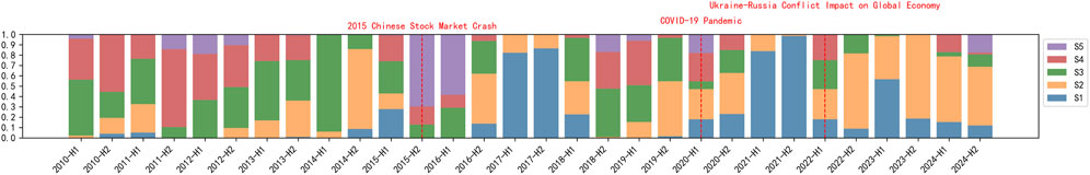
Figure 4. Semiannual market state landscape of Chinese stock market.
3.3 Market states transition
To better understand the dynamic evolution of market conditions, we analyze the empirical transition behavior among the identified market states. Figure 5a presents the empirical state transition matrix of the CSI 300 Index, obtained under the optimal clustering setting
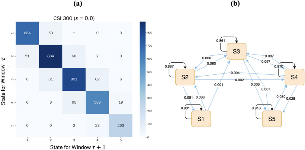
Figure 5. Empirical transition matrix and probabilities among market states.
Figure 5b visualizes the corresponding transition probabilities using a directed graph, where edge annotations indicate the estimated transition probabilities. Most of the mass is concentrated along self-loops and adjacent-state arrows, reinforcing the local stability of market states. Furthermore, the long-run stationary distribution derived from the estimated Markov chain closely aligns with the empirical frequency distribution:
which closely mirrors the empirical frequency of observed states. This consistency reinforces the robustness of the five-state market classification and suggests that the estimated state transitions capture meaningful and persistent structural dynamics in the market.
3.4 Relationship between market states and market crashes
To investigate whether market crashes tend to occur under specific structural states of the market, we examine the relationship between identified market states and empirically observed crash periods. The five market states of the CSI 300 Index are ordered by ascending average pairwise correlation, with the mean correlations given by
Table 1 summarizes the start and end dates of crash episodes, the number of crash cases detected in each episode, the average correlation level during each crash period, and the corresponding market state assigned. These results are based on the proposed crash cases labeling procedure, i. e., Algorithm 2, with time window length
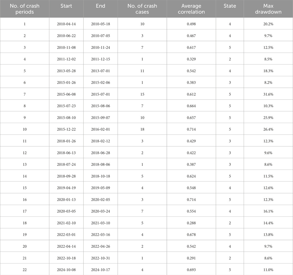
Table 1. Crash period characteristics and corresponding market states.
Based on Table 1, different crash episodes are mapped to different market states, forming an initial distribution of state assignments as
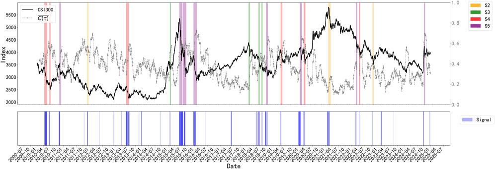
Figure 6. Crash periods and corresponding market states in the CSI 300 Index, along with the rolling forecasting performance of the early warning model. The top panel displays the CSI 300 Index (black) and the average correlation
Overall, the results suggest a strong association between elevated-correlation market states and the occurrence of crashes. In particular, States 4 and 5 appear to signal heightened structural instability. This implies the Markov transition diagram of states in Figure 5b can be served to synchronously monitor the market’s stability status. However, it is important to emphasize that such state classifications should be interpreted as contemporaneous reflections of market conditions, rather than forward-looking predictors. Whether they provide sufficient information for lead time warning is addressed in the following section.
4 Early warning of stock market crashes based on state transition information
This section explores the predictive value of market state transitions in generating early warnings for stock market crashes. Building on the classification framework established in previous sections, we aim to determine whether temporal patterns in market state dynamics can be effectively utilized to identify imminent periods of elevated market risk.
Based on the results in Table 1, we identify a total of 124 crash cases. For each of these, we label the trading day immediately preceding the start of the case as
4.1 Model tuning and implication
To systematically examine how the temporal structure of state-based inputs affects the performance of crash early warning, we adopt the methodology outlined in Section 2.2, varying the window lengths used to construct the three categories of state-derived variables. Specifically, the candidate window lengths
In total, 196 different
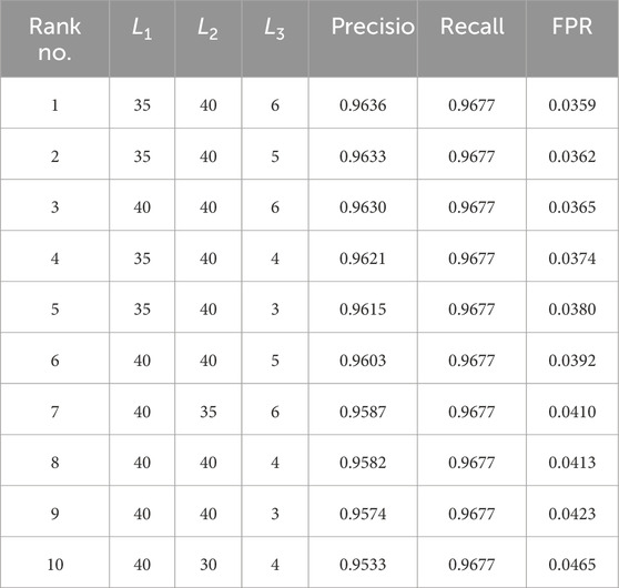
Table 2. Top 10 best feature configurations.
We did not construct a separate test set for final model evaluation. Given the rarity and temporal clustering of crash events, a fixed test split may lead to high variance and unreliable evaluation. Instead, our focus is on examining whether temporal features of market state transitions offer informative signals for early crash detection. In future work, more rigorous backtesting approaches—such as Combinatorial Purged Cross-Validation (CPCV) [31]—could be explored to validate model performance in a production-like environment.
To provide a more detailed and intuitive assessment of how different window length combinations contribute to model performance, we visualize the precision, recall, and F1-score across all 196
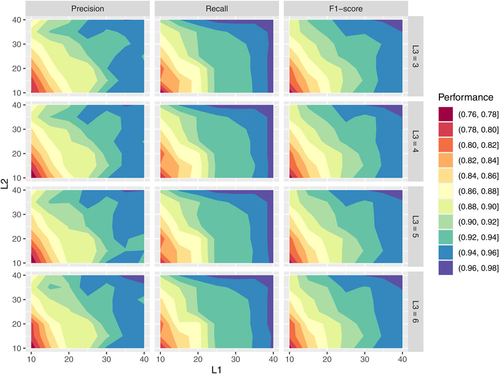
Figure 7. Heatmaps of precision, recall, and F1-Score with hyper-parameters combinations
The heatmaps reveal several consistent patterns. First, larger values of
Figure 8 illustrates the structure of a representative decision tree trained under the optimal window configuration
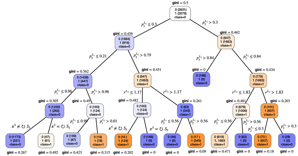
Figure 8. Decision tree structure under the optimal window configuration
Notably, one of the clearest decision paths leading to a crash classification occurs when
To further examine the practical utility of the proposed early warning model, we apply the optimized classifier in a rolling forecasting mode. At each time step, the model uses only past information to predict whether a warning signal should be triggered for the next period. This simulates a realistic deployment setting where market operators make real-time decisions based on evolving structural dynamics. The lower panel of Figure 6 visualizes the resulting forecasted warning signals over the full sample period. Most warnings align closely with the start of crash periods identified by our drawdown-based labeling scheme, often appearing several days in advance. These results confirm that the model generalizes well to unseen data and is capable of generating timely early warnings in real-world settings.
To benchmark the performance of our proposed market state transition (MST) framework, we compare it with three representative baseline models of early warning signals that are widely used in the literature: (1) volatility-based indicators, (2) spectrum-based indicators and (3) absorption ratio.
For the volatility model, we construct a VIX-like indicator based on the implied volatility of the China ETF 50 options, often referred to as the “China fear index.” This index serves as a functional proxy for market-perceived risk in the Chinese context. For the spectrum-based category, we follow the methodology of Chakraborti et al. [20] to compute the maximum eigenvalue of the correlation matrix. For the absorption ratio, we use the implementation proposed by Kritzman et al. [6], which quantifies the proportion of variance absorbed by a fixed number of principal components.
To enable a fair comparison, we construct decision-tree-based classifiers for each of these indicators by tuning thresholds to generate binary crash warnings. All models are evaluated using the same labeled crash dataset and assessed under 5-fold cross-validation. Table 3 presents the results. Our MST-based framework consistently outperforms the benchmark models across all metrics, achieving the highest precision (0.964), recall (0.968), and F1-score (0.966), along with the lowest false positive rate (3.7%). These results highlight the advantage of structurally grounded, transition-driven features in anticipating systemic stress.
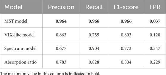
Table 3. Comparison of early warning models using 5-fold cross-validation.
4.2 Adaptability to new data
To evaluate the model’s adaptability in real-time environments, we assess its ability to incorporate newly arriving trading data using the procedure described at the end of Section 2.2. Specifically, new correlation matrices are projected into the original low-dimensional MDS space, and their market state labels are assigned using a Support Vector Machine (SVM) trained on the initial clustering results.
Results from 5-fold cross-validation indicate that the SVM with a radial basis function (RBF) kernel achieves a classification accuracy of 98.20%, demonstrating that new trading days can be accurately labeled with minimal computational cost. This confirms the model’s suitability for real-time deployment and continuous market monitoring under dynamic conditions.
4.3 Sensitivity analysis
To evaluate the robustness of our results with respect to key design choices, we conduct two sets of sensitivity analyses focusing on crash labeling and resampling methods.
First, we examine the impact of changing the drawdown threshold
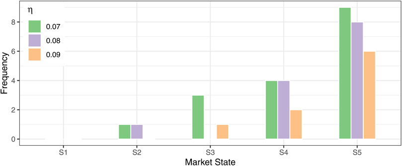
Figure 9. Sensitivity of crash-state distribution to drawdown threshold
Second, we assess the influence of different resampling techniques used to address class imbalance in model training. In addition to the simple replication method (Simple Rep) used in the main analysis, we consider two widely used alternatives: SMOTE and ADASYN. As shown in Figure 10, the decision tree model maintains stable performance across all three approaches. While SMOTE and ADASYN yield slightly lower precision, recall and F1-score, the overall differences are modest, supporting the validity of our original choice. These results demonstrate that the predictive effectiveness of our framework is not materially dependent on the specific sampling method adopted.
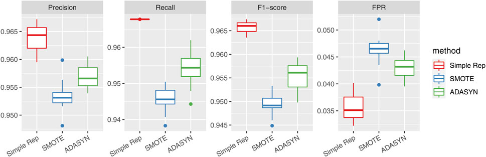
Figure 10. Model performance under different resampling methods. Bars represent precision, recall, F1-score, and false positive rate (FPR) for simple replication, SMOTE, and ADASYN. The results demonstrate that the model’s performance remains stable across various class-balancing strategies.
5 Conclusion
Grounded in the complex systems perspective, this paper applies correlation-based structural analysis to identify and characterize market states in the Chinese stock market, with the CSI 300 Index as a representative system. Using multidimensional scaling and K-means clustering on rolling correlation matrices, we identify five distinct market states that reflect varying levels of systemic co-movement. Our analysis confirms that these states are not merely statistical artifacts but correspond to meaningful structural configurations of the market.
Empirical results reveal that market state transitions are predominantly local, occurring between adjacent states, while abrupt multi-level jumps are rare. States also exhibit high temporal persistence, underscoring the gradual and inertial nature of structural evolution in financial systems. Notably, high-indexed states—those with elevated average correlations—are strongly associated with historically observed crashes, particularly when the market resides in State 4 or State 5, where systemic co-movement is most pronounced. While these states offer valuable insight into ongoing market fragility, they function primarily as contemporaneous indicators rather than forward-looking predictors. Together, these findings support the use of market state classification as a structurally grounded, real-time measure of systemic risk.
Based on the identified state structure, an early warning model is constructed using decision trees trained on state-derived temporal features. These features capture medium-term structural distributions, directional trends in state transitions, and recent evolutionary patterns. The model demonstrates high recall and precision across multiple validation settings, indicating strong robustness in identifying pre-crash conditions. Furthermore, real-time adaptability is ensured through a projection-based labeling procedure, allowing new data to be efficiently embedded and classified, thus enabling continuous and responsive market surveillance.
Several avenues for future research emerge from this work. One direction is to extend the proposed framework to cross-market or multi-asset systems, such as incorporating global indices, fixed income instruments, or cryptocurrency markets, to examine whether state transitions exhibit comparable structural patterns across different financial domains. Another promising line lies in enriching the modeling of state transitions themselves—e.g., using recurrent neural networks to capture nonlinear memory effects. Furthermore, combining structural state dynamics with behavioral signals, news flows may enhance the predictive power and interpretability of crash warnings. Finally, linking market state trajectories with macro-financial policy variables could offer new insights into the interplay between systemic risk and regulatory interventions.
Data availability statement
The original contributions presented in the study are included in the article/Supplementary Material, further inquiries can be directed to the corresponding author.
Author contributions
W-YP: Data curation, Formal Analysis, Software, Visualization, Writing – original draft. LL: Conceptualization, Investigation, Methodology, Project administration, Software, Supervision, Validation, Visualization, Writing – original draft, Writing – review and editing.
Funding
The author(s) declare that financial support was received for the research and/or publication of this article. We acknowledge financial support from the National Natural Science Foundations of China (Grant No. 71771086).
Conflict of interest
The authors declare that the research was conducted in the absence of any commercial or financial relationships that could be construed as a potential conflict of interest.
Generative AI statement
The author(s) declare that no Generative AI was used in the creation of this manuscript.
Publisher’s note
All claims expressed in this article are solely those of the authors and do not necessarily represent those of their affiliated organizations, or those of the publisher, the editors and the reviewers. Any product that may be evaluated in this article, or claim that may be made by its manufacturer, is not guaranteed or endorsed by the publisher.
Supplementary material
The Supplementary Material for this article can be found online at: https://www.frontiersin.org/articles/10.3389/fphy.2025.1647667/full#supplementary-material
References
1. Sornette D. Why stock markets crash: critical events. In: Complex financial systems. 2nd edn. Princeton, NJ: Princeton University Press (2017).
2. Mantegna RN, Stanley HE. Introduction to econophysics: correlations and complexity in finance. Cambridge University Press (2000).
3. Bouchaud J-P. The (unfortunate) complexity of the economy. Phys World (2009) 22:28–32. doi:10.1088/2058-7058/22/04/39
4. Hommes C. Complex evolutionary systems in behavioral finance. In: Handbook of financial markets: dynamics and evolution. Elsevier (2009). p. 217–76.
5. Münnix MC, Shimada T, Schäfer R, Leyvraz F, Seligman TH, Guhr T, et al. Identifying states of a financial market. Scientific Rep (2012) 2:644–6. doi:10.1038/srep00644
6. Kritzman M, Li Y, Page S, Rigobon R. Principal components as a measure of systemic risk. The J Portfolio Management (2011) 37:112–26. doi:10.3905/jpm.2011.37.4.112
7. Billio M, Getmansky M, Lo AW, Pelizzon L. Econometric measures of connectedness and systemic risk in the finance and insurance sectors. J Financial Econ (2012) 104:535–59. doi:10.1016/j.jfineco.2011.12.010
8. Lin L, Sornette D. “speculative influence network” during financial bubbles: application to Chinese stock markets. J Econ Interaction Coord (2018) 13:385–431. doi:10.1007/s11403-016-0187-7
9. Lin L, Guo X. Identifying fragility for the stock market: perspective from the portfolio overlaps network. J Int Financial Markets, Institutions Money (2019) 62:132–51. doi:10.1016/j.intfin.2019.07.001
10. Sandhu R, Georgiou T, Tannenbaum A. Ricci curvature: an economic indicator for market fragility and systemic risk. Sci Adv (2016) 2:e1501495. doi:10.1126/sciadv.1501495
11. Samal A, Pharasi HK, Ramaiah SJ, Kannan H, Saucan E, Jost J, et al. Network geometry and market instability. R Soc Open Sci (2021) 8:rsos.201734. doi:10.1098/rsos.201734
12. Scheffer M, Bascompte J, Brock WA, Brovkin V, Carpenter SR, Dakos V, et al. Early-warning signals for critical transitions. Nature (2009) 461:53–9. doi:10.1038/nature08227
13. Hoel EP. When the map is better than the territory. Entropy (2017) 19:188. doi:10.3390/e19050188
14. Chen M, Li N, Zheng L, Huang D, Wu B. Dynamic correlation of market connectivity, risk spillover and abnormal volatility in stock price. Physica A: Stat Mech Its Appl (2022) 587:126506. doi:10.1016/j.physa.2021.126506
15. Wu B, Huang D, Chen M. Estimating contagion mechanism in global equity market with time-zone effect. Financial Management (2023) 52:543–72. doi:10.1111/fima.12430
16. Yu D, Huang D. Cross-sectional uncertainty and expected stock returns. J Empirical Finance (2023) 72:321–40. doi:10.1016/j.jempfin.2023.04.001
17. Pharasi HK, Sharma K, Chatterjee R, Chakraborti A, Leyvraz F, Seligman TH Identifying long-term precursors of financial market crashes using correlation patterns. Physica A: Stat Mech its Appl (2018) 516:603–16.
18. Heckens A, Guhr T. A new attempt to identify long-term precursors for financial crisis in the market correlation structures. arXiv preprint (2021).
19. Pharasi HK, Sharma K, Chakraborti A. Dynamics of market states and risk assessment. Physica A: Stat Mech its Appl (2024) 631:129191.
20. Chakraborti A, Sharma K, Pharasi HK. Phase separation and scaling in correlation structures of financial markets. J Phys Complexity (2020) 2:015002. doi:10.1088/2632-072x/abbed1
21. Chetalova D, Schäfer R, Guhr T. Zooming into market states. J Stat Mech Theor Exp (2015) 2015:P01029. doi:10.1088/1742-5468/2015/01/p01029
22. Spelta A, Flori A, Pecora N, Buldyrev S, Pammolli F. A behavioral approach to instability pathways in financial markets. Nat Commun (2020) 11:1707–9. doi:10.1038/s41467-020-15356-z
23. Begušić S, Kostanjčar Z, Kovač D, Stanley H, Podobnik B. Information feedback in temporal networks as a predictor of market crashes. Complexity (2018) 2018:1–13. doi:10.1155/2018/2834680
24. Wang X, Zhao L, Zhang N, Feng L, Lin H. Stability of China’s stock market: measure and forecast by ricci curvature on network. Complexity (2023) 2023:1–12. doi:10.1155/2023/2361405
25. Xing K, Yang X. How to detect crashes before they burst: evidence from Chinese stock market. Physica A: Stat Mech Its Appl (2019) 528:121392. doi:10.1016/j.physa.2019.121392
26. Cerqueti R, Gatfaoui H, Rotundo G. Resilience for financial networks under a multivariate garch model of stock index returns with multiple regimes. Ann Operations Res (2024). doi:10.1007/s10479-023-05756-x
27. Lim B, Zohren S, Roberts S. Detecting changes in asset co-movement using the autoencoder reconstruction ratio. arXiv preprint arXiv:2002.02008 (2020).
28. Guhr T, Kälber B. A new method to estimate the noise in financial correlation matrices. J Phys A: Math Gen (2003) 36:3009–32. doi:10.1088/0305-4470/36/12/310
29. Burnham KP, Anderson DR. Model selection and multimodel inference: a practical information-theoretic approach. 2nd edn. Springer (2004).
30. Chakraborti A, Sharma K, Pharasi HK. Characterization of catastrophic instabilities: market crashes as paradigm. arXiv preprint (2018).
Keywords: market state transition, systemic risk, early warning, correlation structure, stock market
Citation: Pang W-Y and Lin L (2025) Market state transitions and crash early warning in the Chinese stock market. Front. Phys. 13:1647667. doi: 10.3389/fphy.2025.1647667
Received: 16 June 2025; Accepted: 07 July 2025;
Published: 07 August 2025.
Edited by:
Ze Wang, Capital Normal University, ChinaReviewed by:
Shijia Song, Chongqing University, ChinaLuiz De Jesus, Loyola Andalusia University, Spain
Difang Huang, Chinese Academy of Sciences (CAS), China
Copyright © 2025 Pang and Lin. This is an open-access article distributed under the terms of the Creative Commons Attribution License (CC BY). The use, distribution or reproduction in other forums is permitted, provided the original author(s) and the copyright owner(s) are credited and that the original publication in this journal is cited, in accordance with accepted academic practice. No use, distribution or reproduction is permitted which does not comply with these terms.
*Correspondence: Li Lin, bGxpbkBlY3VzdC5lZHUuY24=