Your new experience awaits. Try the new design now and help us make it even better

ORIGINAL RESEARCH article

Front. Phys., 26 August 2025

Sec. Social Physics

Volume 13 - 2025 | https://doi.org/10.3389/fphy.2025.1648895

This article is part of the Research TopicInnovative Approaches to Pedestrian Dynamics: Experiments and Mathematical ModelsView all 4 articles

Mean-field and Monte Carlo analysis of multi-species agent dynamics

  • Instituto de Física, Universidade Federal do Rio Grande do Sul, Porto Alegre, Brazil

We propose a mean-field (MF) approximation as a recurrence relation governing the dynamics of m species of particles on a square lattice. We simultaneously perform Monte Carlo (MC) simulations under identical initial conditions to emulate the intricate motion observed in environments such as subway corridors and scramble crossings in large cities. Each species moves according to transition probabilities influenced by its respective static floor field and the state of neighboring cells. To illustrate the methodology, we analyze statistical fluctuations in the spatial distribution for m=1, m=2, and m=4 and for different regimes of average density and biased movement. A numerical comparison is conducted to determine the best agreement between the MC simulations and the MF approximation considering a renormalization exponent β that optimizes the fit between methods. Finally, we report a phenomenon we term “Gaussian-to-Gaussian” behavior, in which an initially normal distribution of particles becomes distorted due to interactions among same and opposing species, passes through a transient regime, and eventually returns to a Gaussian-like profile in the steady state, after multiple rounds of motion under periodic boundary conditions.

1 Introduction

Pedestrian dynamics is one example of complex systems of self-driven agents in the realm of macro-scale physics, which give rise to a variety of emerging phenomena. Several theoretical and experimental studies have been conducted on crowd dynamics, focusing on topics ranging from city planning [1] and disaster prevention to the understanding of complex human behavior [2, 3].

Some places with crowd formation as subway corridors [4, 5], nightclub dynamics [6, 7], and scramble crossings [8] in large cities, are examples of these complex systems that exhibit collective behavior. Simply put, it features different groups of individuals aiming to reach various common destinations, for instance, the entrance/exit of a train station, reaching/leaving the bar to buy beverages, or crossing to get to another corner. Thus, the spatial and temporal context in question may involve a single group of agents moving towards a common goal, or multiple groups moving along confronting trajectories, which rapidly increases the complexity of the dynamics.

The problem of two groups of particles in counterflow has been extensively studied across various contexts, ranging from microscopic scales—such as the dynamics of charged colloids [9]—to macroscopic phenomena, such as pedestrian flows in corridors [10, 11], and even more complex situations like evacuation [12] scenarios. Notably, even in single-species models [13], intriguing phenomena such as condensate formation emerge, illustrating the richness of these systems.

An interesting approach to describe the hard-body dynamics of macroscopic systems is the lattice-gas modelling [14]. In our recent work, we used the dynamics of a lattice gas-type interaction to describe the motion of pedestrians inside nightclubs [6, 7] and in a four-way crossing walk [8], the so-called scramble crossing. In such works, we have shown that the intrinsic high correlation of this approach reflects the model’s sensitivity to jamming and condensate formation.

In that sense, Monte Carlo (MC) simulations are a natural method for studying such models, as they allow for the definition and implementation of transition rules to simulate different evolutions from specified initial conditions. These systems can also be interpreted in a broader context as multi-agent systems. Additionally, there are approaches that model these dynamics through differential equations based on Newton’s laws, within the so-called social force framework [12, 15, 16].

In that direction, the mean-field (MF) approach in particle dynamics has been extensively studied, particularly in the context of lattice gas models. These models were originally proposed to describe the behavior of specific types of fluids, such as solvents [17], electrochemical cells [18], and other systems that can be characterized by Hamiltonians derived from free energy potentials [19]. In 2015, we introduced a related model [20] based on a two-species particle framework to describe pedestrian counterflow. Unlike classical exclusion principles, our model employed density-dependent exclusion rules, where the probability of occupation varied with the local density of particles. The system’s evolution was governed by a set of coupled partial differential equations (PDEs). Other variations have been explored to model deterministic dynamics [21, 22], and further extensions of our framework have incorporated concepts from Fermi-Dirac statistics [23].

In this work, we propose a general framework for a MF approximation of the lattice gas dynamics of m-species of particles on a square lattice. We derive a generalized non-linear coupled PDE obtained by the MF approximation and compare it to MC simulations, by using a set of initial conditions for the cases m=1, m=2, and m=4, where each type of particle is guided by its own static floor field [24] towards its target. We study the statistical properties of the distributions of particles of the species and investigate what are the circumstances and range of parameters that make the model a suitable and efficient option for MC simulations.

Our results show excellent agreement between the PDE predictions and MC simulations for low-density regimes. However, at higher densities, jamming effects reduce the accuracy of this agreement. We present a detailed numerical study to delineate the conditions under which our method remains valid compared to the computationally more expensive MC simulations.

In the next section, we describe the method for deriving the PDEs based on a model where particles exhibit preferential directed motion combined with random movements dependent on the occupation of neighboring sites. Through a mean-field approximation, we successfully derive a generalized PDE that describes scenarios involving an arbitrary number m of species.

Subsequently, in the third section, we present our results comparing the spatial distribution of particles on a bidimensional lattice for different model parameters and initial particle concentrations. We study three different cases —m=1, m=2, and m=4—, analyzing the evolution of key distribution features over time under periodic boundary conditions. These features reflect the interactions between particles across the various scenarios. Additional details—including equation derivations, supplementary plots, and a discussion of numerical instabilities related to the PDEs—are provided in the supplemental material accompanying this text.

2 Methods

Our model consists of a system of n particles that move along an underlying square lattice of side l. Each particle in the system belong to one of m species and can hop to one of its first neighboring cells at each time step according to a set of transition probabilities which depends on its species “social fields” (static floor field), denoted as u(k)=u(k)(r), where k=1,,m. For instance, a given particle belonging to the species q at cell r=(i,j) hops to one of its neighboring cells r=(i,j) in the unit time interval tt+1 according to the transition probability density

Prrrq=p+αΔrûq,(1)

where p is a constant probability to hop to one of the four neighboring cells, α is the coefficient that measure the bias towards the direction of its species static floor field, û(q)u(q)/u(q) is the normalized static floor field of species q, and Δrrr is the displacement vector of the calculated transition probability. As one may expect, normalization constraints reflect on the possible values of p, which in a Cartesian regular lattice is 0<p1/4, whilst α satisfies the condition 0<αp.

It is important to note that, in our model, each particle perceives only the static floor field specific to its species, evaluated at its current position. Consequently, the inner product defined in Equation 1 quantifies the contribution of each possible transition probability to the particle’s movement toward its target.

As one might anticipate, Equation 1 is the general form of the four possible transition probabilities each of which have a different corresponding displacement vector that can assume the values Δr=ex, ex, ey, and ey, with ex and ey denoting the unit vectors of our reference frame as depicted in Figure 1. Thus, to ensure the normalization constraint, the probability that a particle remains in its current cell is expressed as:

Prrrq=1rPrrrq=14p,(2)

where the angle brackets r indicate that the summation is carried out solely over the nearest neighbours, with i=i±1 and j=j±1.

Figure 1
Graph showing a grid with axes labeled x and y, with several grid lines marked with variables i, j, and increments. Two vectors, r and r', are drawn from the origin to points on the grid, with vector r' being displaced by Δr.

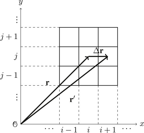
Figure 1. Cartesian lattice depiction of a likely transition to happen of a particle at position r to a neighbouring cell r=r+Δr.

It is important to note that these transition probabilities define the intended particle movement, conditional on the target cell being empty, as each cell can accommodate at most one particle. Thus, the probability represents what should occur, not what will necessarily occur.

2.1 Lattice gas dynamics

We focus our study on an approximate regime of a lattice gas model. The key feature, as previously noted, is the exclusion principle, which prevents particles from overlapping or occupying the same cell, regardless of the specific rules governing the transition probabilities. This characteristic makes it particularly challenging to derive an approximate recurrence relation or equation of motion, as the occupation states of neighboring lattice cells are highly correlated. Nevertheless, we develop a recurrence relation for the cell occupation that remains consistent with the asynchronous updating scheme characteristic of lattice gas dynamics with nearest-neighbor interactions. Accordingly, we propose the following recurrence relation for a given species q:

ρt+1qr=1ρtrrρtqrPrrrq+ρtqrPrrrq+rρtrPrrrq,(3)

where ρt(r)k=1mρt(k)(r) is the total density of particles at a given cell r at time step t. The proposed equation decomposes the update process into two key contributions: (1) particle inflow into the cell and (2) particle persistence or outflow from the cell. In the lattice gas dynamics, the occupation state is binary, with ρt(q)(r)=1 if the cell is occupied and ρt(q)(r)=0 if it is vacant. However, in the mean-field (MF) approximation, ρt(r) represents an average density field and does not directly reflect the actual number of particles n in the system. To bridge this gap and improve consistency between the MF and MC descriptions, we generalized the normalization condition of the MF recurrence relation. Specifically, we modified the global constraint so that the sum over all lattice sites scales as a power of n:

rρtr=nβ,

where β is a tunable exponent. The introduction of β allows us to adjust the MF approximation to better reproduce the behavior observed in MC simulations. By treating β as a fitting parameter, we aim to compensate for the differences between the averaged MF treatment and the discrete, stochastic nature of the MC dynamics.

The first term on the right-hand side of Equation 3, the factor 1ρt(r), reflects the hard-body exclusion principle, which dictates that a particle can only occupy an empty cell. This factor multiplies the sum of possible sources of inflow of particles of species q from the neighboring cells of r, i.e., the notation r. Each neighboring source of particles depends on the density of the species q at the neighboring site ρt(q)(r) and the transition probability Prrr(q), reflecting its likelihood to hop from r to r. The second term on the right-hand side of Equation 3 describes the contribution of particles already present in r. The first factor, ρt(q)(r), accounts for the actual occupation of it, whilst the factor inside the large brackets corresponds to a composition of two possibilities. The first possibility is the probability Prrr(q) of the particle at r remaining in place, which contrasts with the second possibility that stands as the probability of the particle at r trying to move to an occupied neighboring cell r.

With this framework, we explicitly separate the exclusion interaction, reflected in the terms 1ρt(r) and ρt(r), from the transition probabilities, which can incorporate additional interaction mechanisms such as long-range fields or cooperative dynamics. As an example, Equation 3 can reproduce even deterministic models of particles, such as proposed in [21], which could allow us to describe the model proposed by Cividini et al., for instance, by a proper choice of parameters such as fixing m=2 with one species moving eastbound and the other species moving northbound with transition probabilities equal to one towards their respective target directions.

We can rewrite Equation 3 as follows

ρt+1qr=rωtqr,rωtqr,rρtrωtqr,rρtrωtqr,r+ρtq,(4)

where ωt(q)(r,r)ρt(q)(r)Prrr(q) is the flow rate of particles of species q entering the cell at r from the cell r. Alternatively, we could write Equation 4 as

ρt+1qr=ΦtqrΨtqr+ρtq,(5)

where

Φtqrrωtqr,rωtqr,r(6)

is the net flow rate of particles of species q into the cell at r and

Ψtqrrρtrωtqr,rρtrωtqr,r(7)

is the frustrated net flow rate of particles of species q into the cell at r. The frustrated net flow rate measures the particle interaction, i.e., measures the amount of q particles unable to access or leave the cell at r due to the its occupation and of its neighbouring cells Equations 5-7 provide an alternative representation that offers a more physical perspective on the mean-field dynamics.

2.2 Mean-field regime

When applying Equation 1 into the lattice gas recurrence relation given by Equation 3, we end up with the specific recurrence relation

ρt+1qr=1ρtrrρtqrpαΔrûqr+ρtqr14p+rρtrp+αΔrûqr.(8)

After some algebra (see Supplementary Material A) we obtain the following partial differential equation

ρqt=c12ρqc2ρqûqc3kqρk2ρqρq2ρk+c4k=1mρkρqûq+ρqρkûq,(9)

where c1,c3limτ,ϵ0pϵ2τ and c2,c4limτ,ϵ0αϵτ.

In Equation 9, we notice that the constants c3 and c4 are species’ coupling factors and the mathematical path we took from Equation 3 makes them not to depend on each possible pair of species. However, a more general approach would consider these constants as dependent on each possible coupling pair of species, which we will not going to explore in this work.

To study how good a fit is the mean-field approximation is to the particle dynamics, we investigate how the spatial distributions of both methods differ from each other for different sets of the model parameters such as the total number of particles (n), the total number of species (m), and the bias level of movement (α).

3 Discussion

As mean-field approaches approximate the microscopic behavior to an average behavior, their fidelity to the model tends to be limited to a certain range of parameters. This restriction is potentiated when considering cases of highly correlated systems of particles, such as the lattice gas dynamics we study in this work. In particular, we addressed how a system of an arbitrary number of species m, each carrying a different static and uniform social field u, influences emerging phenomena. As stated previously, the social field’s direction is the only cause of difference between particles of different species, so that a system of m>1, but with u(1)=u(2)==u(m) is not different from the case m=1. In that sense, the complexity of the model comes from different configurations of static floor fields.

Thus, to simplify things a little bit, we use a relatively simple rule to define social fields û(q), where each species has a guaranteed different field from each other in the two-dimensional Cartesian lattice:

ûq=cos2πq1m,sin2πq1m.(10)

By defining the static floor fields in Equation 10 as such, we took the first species to have its preferential direction of movement parallel to the x-axis, whilst all other species’ directions are defined in regularly divided angles according to the total number of particles (m).

As initial conditions, we considered each species concentrated in separate regions of the lattice as initial “wave packages” to describe what would be a real physical confrontation scenario, such as found in pedestrian crossings [8, 21]. More specifically, we considered each species’ initial distribution as a bivariate uncorrelated normal distribution with mean values defined in a circular fashion analogous to the static floor fields previously defined with a light difference. To observe confrontation between species, we defined the initial distributions of each as μx(q)=l2112cos2π(q1)m and μy(q)=l2112sin2π(q1)m. That particular choice guarantees that agents will have to cross each other at the lattice center, simulating scenarios where species have well-defined positions and confrontation between groups of agents with different objectives is bound to occur as depicted in Figure 2.

Figure 2
Graph showing a circular arrangement with black dots connected by blue arrows pointing inward. Axes are labeled x and y, with values and expressions like \( \frac{m}{4} \), \( \frac{l}{2} \), and similar increments. The circle is dashed, featuring expressions around its perimeter, such as \( \frac{3m}{4} + 1 \) and \( \frac{m}{2} - 1 \).

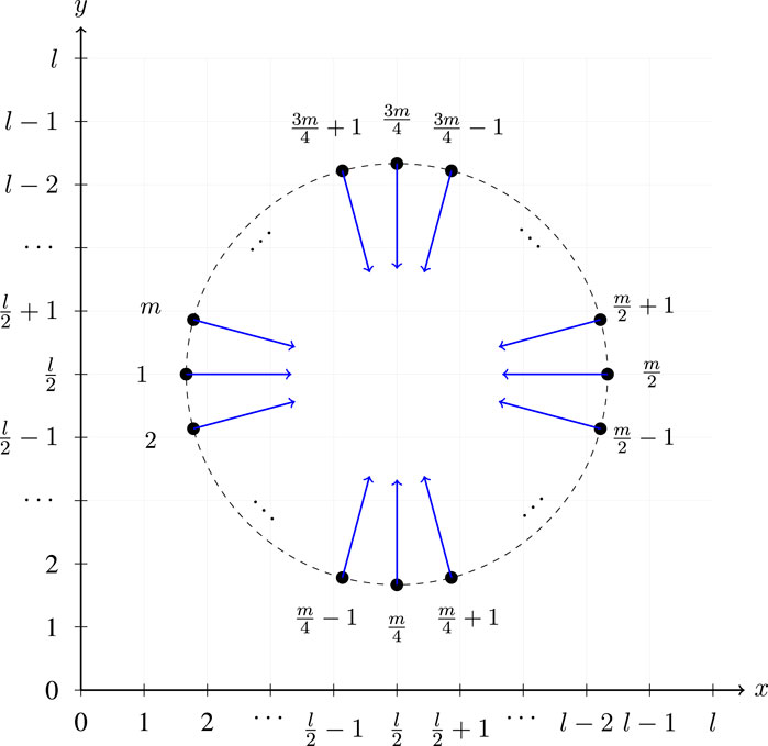
Figure 2. Schematic lattice (not to scale) illustrating a system with m species in a situation involving confrontation. Each point marks the mean μx(q),μy(q) of a species’ initial distribution, with arrows indicating the direction of its static floor field. Angular separations are illustrative; actual values depend on m. The figure conveys the structure of initial conditions and static fields.

For all species, we define the standard deviation of the initial distributions to be σx(q)=σy(q)=l/32. The reason behind this specific choice for the standard deviation and not a smaller value is the constraint of the exclusion feature of the lattice model. For instance, a Dirac’s delta function as initial distribution, where σx(q)=σy(q)0, can only be implemented on MC simulations if we put only one particle in the species mean initial position and we would have to make the system large enough so to have an approximate distribution of choice, which would be impractical computationally. In that sense, to study systems with more than one particle per species, we have to choose initial distributions not so localized.

Specifically, we have examined the cases of m=1, m=2, and m=4, which represent simpler scenarios where the species’ static floor fields align with the x- and y-axes. This alignment with the Cartesian axes provides a symmetric structure that facilitates a clearer comparison between the two methods via the marginalized distribution relative to the species’ static floor field. For instance, if a species has a preferred direction û=±ex, we compute the marginalized density ρ(x) by summing ρ(x,y) over all y-values. This reduction to a one-dimensional distribution simplifies the analysis.

In all cases, we studied a system of l=128 with periodic boundary conditions on both directions (toroid). In a previous study, we performed a finite-size scaling analysis of the three-species version of this model using an indirect observable—the bar profits (see Ref. [6]). The results indicated that a lattice size of l=128 was sufficiently large to suppress boundary effects. We also used p=1/4 in this work, which reflects a scenario of high noise dynamics (see Equation 2) where particles only stay still if the target cell is occupied.

We simulated the particle dynamics of our model via MC algorithm with a shuffled asynchronous update scheme. This means that at any given MC step, we form a list of n particles chosen at random (uniform distributed pseudo-random number generator [25]) from the population of n that compose the system. We then update the position of each sequentially, according to the transition probabilities given by Equations 1, 2 and its neighboring cell states. For the initial conditions, we used a Box-Muller algorithm [25] to generate two independent and normally distributed pseudo-random variables (X and Y) to define each particle’s position according to their species. Throughout this work, variables originating from MC simulations were obtained by averaging the time series of each run at each timestep over nrun=106/n samples generated with same parameter, but different seeds for the pseudo-random number generators.

3.1 m=1 case

The simplest scenario we examined involves only a single species. As we defined previously by Equation 10, a single species tends to move according to the static floor field û=ex, with its initial distribution having μx(1)=l/4 and μy(1)=l/2 with σx(q)=σy(q)=l/32. In these simulations, we used β=1.

In Figure 3, we present plots of the marginal distribution of particles along x, where circles represent the Monte Carlo (MC) simulation results and solid lines correspond to predictions from the recurrence relation (mean-field approximation). We examine these distributions for various particle counts, ranging from n=64 to n=448 in increments of Δn=64 and shown at four distinct time steps: (a) t=50, (b) t=250, (c) t=450, and (d) t=4950. For this study, we used α=0.15, which corresponds to agents with mid range level of impetus as we already shown in [7, 8].

Figure 3
Eight graphs show probability density functions with various parameters. Graphs (a), (b), (c), and (d) on the top row depict density distribution for different sample sizes: 64, 128, 192, and 256. Graphs (e), (f), (g), and (h) on the bottom row illustrate distribution with different alpha values: 0.050, 0.150, and 0.200. Each graph plots \(x'\) on the horizontal axis and \(\rho(x')\) on the vertical axis, showing overlapping curves in different colors.

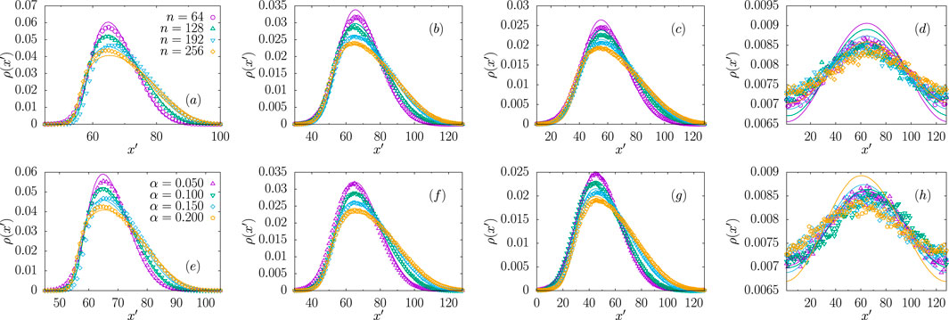
Figure 3. Evolution of normalized marginal distributions of x of MC simulations (circles) and MF (lines) for different time steps (a,b) t=50, (b,f) t=250, (c,g) t=450, and (d,h) t=4950 considering one-species (m=1). Plots labeled from (a-d) illustrate the influence of different values of n for a fixed α=0.15, whereas plots from (e-h) show the effect of varying α for a fixed n=192.

As a general remark, we notice a qualitatively good agreement between the two methods and that the distributions in more densely populated systems shows more positive skewness of the probability density function (PDF) in comparison to systems with fewer particles, revealing the exclusion effects. These exclusion effects are a result of agents leading the pack acting as obstacles for the particles in the bulk. As time passes, we notice that the distributions present increasing dispersion with the “front tail” maintaining synchronicity for different values of n. It is important to disclose that in the study that produced Figure 3, the recurrence relation exhibited numerical instability for n512, which the corresponding data is omitted here and throughout the manuscript for conciseness. To understand the source of the instabilities, note that Equation 8 includes the term 1ρt(r), which, in the context of discrete particle dynamics, only takes values 0 or 1, as previously explained. In this regime, the factor 1ρt(r) behaves in a stable and well-defined manner. However, under the mean-field approximation, increasing either the total density N/V or the parameter α can lead to locally high average densities. As a result, 1ρt(r) may become negative, causing ρt+1(r) to also take on unphysical negative values. When this occurs, the normalization of the distribution becomes unstable, as the sum involves both large positive and negative terms—sometimes yielding normalized values with magnitudes as high as 1020. Thus, providing a quantitative indication that there exists a certain range of the parameters of the model beyond which the approximate method becomes unreliable and serves as justification for the assumption that a tuning parameter, β, might be necessary to also preserve the mean-field stability. The reader is advised to check the supplementary material to check the form of marginal distributions of particles right before numerical collapse.

Another key parameter we investigated is the bias movement level, α, which quantifies the particles’ tendency to move in their species’ preferred direction. For this analysis, we fixed n=192, corresponding to a generally low-density scenario as shown, while ensuring sufficient particle interactions to produce the positive skewness observed in the distribution.

In the lower panels of Figure 3 (plots e to h), we present the marginal distributions at time steps (e) t=50, (f) t=250, (g) t=450, and (h) t=4950 for α=0.050,0.100,0.150, and 0.200. As expected, distributions with higher α values exhibit faster drift velocities in the +x direction. Additionally, increasing α amplifies the skewness, similar to the effect observed with higher n. Notably, at longer simulation times, larger α values lead to greater discrepancies between the two methods, as seen in Figure 3h.

Given the phenomena observed in Figure 3, we notice that systems with a greater total number of particles (n) tend to show less agreement, even if qualitatively their shapes follow the same pattern. However, this disparity is not observed when changing the level of movement bias (α) shown in Figure 3. With this in mind, we show, in Figure 4, how the exponent of normalization, β, influences the shape of the marginal distribution of x.

Figure 4
Four-panel chart depicting various data visualizations. Panel (a) shows a line graph of ρ(x) against x for different β values, indicating peaks around x=50. Panel (b) presents ΔS² against β for different n values, each line decreasing sharply near β=1. Panel (c) displays a scatter plot with a regression line for βc against n, showing a decreasing trend. Panel (d) compares data and fits for βc against n with m=2 and m=4, both showing similar downward trends.

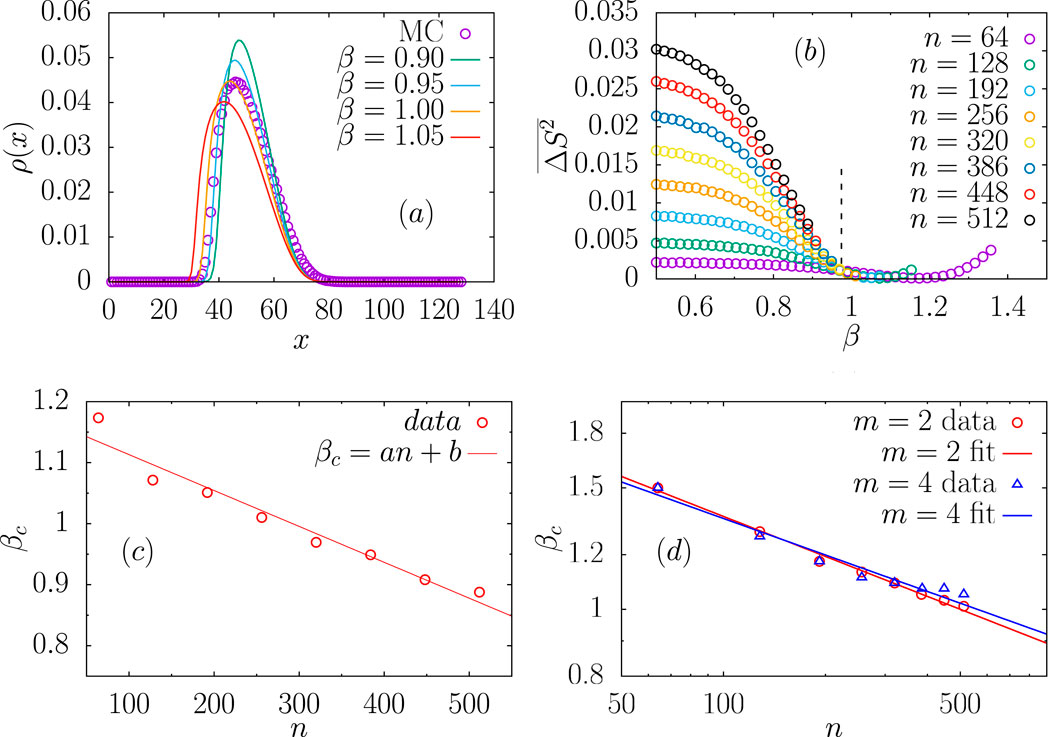
Figure 4. (a) Influence of β on the distribution profile for a system with parameters m=1, n=128, and α=0.249. (b) Variation of the average squared deviation ΔS2̄ as a function of β, for a single-species system (m=1) with α=0.15. (c) Completing the analysis for m=1, we show the linear dependence of the optimal value βc on the number of agents. The data is fitted with a linear function ax+b, yielding a=0.000588±5.3×10⁵ and b=1.17±0.017. (d) By extending the same calculations to systems with multiple species (m=2 and m=4), we observe that the results are well described by power function fits for βc, using the form axb. The fitted parameters are: m=2: a=3.3±0.11, b=0.193±0.0065; m=4: a=3.04±0.23, b=0.176±0.014.

Figure 4a illustrates the influence of β on the distribution profile for a system with parameters m=1, n=128, and α=0.249. As discussed in the previous section, the normalization constraint in the recurrence relation can be interpreted through an ansatz in which the number of particles is raised to a power β, with β expected to be close to 1, if not exactly 1. As such, this parameter serves to tune the agreement between methods at the same time, it allows for systems with number of particles expected to show numerical collapse to evolve in a well-behaved manner.

To better measure the agreement between the two methods and the range of parameters where the mean-field shows numerical stability, we compared both methods using the time average of the squared difference of the spatial entropies of each method, i.e.,

ΔS2̄1tmaxt=1tmaxStMCStMF2,(11)

where St=rρt(r)lnρt(r). The loss function introduced in Equation 11 is one among several possible choices for quantifying the discrepancy between the MC and MF results. However, as we demonstrate below, it proved to be particularly suitable for optimization purposes. For comparison, we also tested an alternative loss function based on the squared differences of local densities, as illustrated in Supplementary Figure S2 and defined in its caption in the Supplementary Material. This alternative metric failed to produce a well-behaved optimization landscape, which made it ineffective for identifying optimal values of β. For this reason, we opted not to pursue it further.

In Figure 4b, we show ΔS2̄ as a function of the exponent β for different values of n and for a fixed simulation time of tmax=104 time steps. We studied the range of β[0.5:1.5]. In this range, we observed numerical instability of the recurrence relation in all curves shown for values of β greater than certain values, which are reflected by the discontinuity of the curves. More specifically, greater n shows lower β’s where the numerical collapse occurs. However, within the range of numerical stability, we observe that, for n256, methods show an optimal agreement at ββc>1, shown by the local minima which become closer to 1 as n increases. For n256, we notice that the numerical instability of the MF makes the lowest stable β assume the stance of optimal value, i.e., it becomes the value that minimizes ΔS2̄.

Figure 4c completes the analysis for m=1, by showing the linear dependence of the optimal value βc on the number of agents. The data is fitted with a linear function ax+b, yielding a=0.000588±5.3×10⁵ and b=1.17±0.017. Such behavior will be different of upper values of m as it is previously presented in Figure 4d. However, we must first study the particle distribution for these cases under varying parameters, which will be performed in the next sections.

3.2 m=2 case

The case m=2 is the simplest case within our proposed framework of initial conditions (see Figure 2) where two species of particles move in counterflow, which is a scenario vastly studied in the literature, once it can describe a two species systems with opposing responses to an external field such as oppositely charged coloids [9, 20] (external electrical field) or chromatographic columns [10, 2629] (gravitational field), to cite a few. For this case, initial distributions assume μx(1)=l/4 and μy(1)=l/2, μx(2)=3l/4 and μy(2)=l/2 as we defined in the previous section. Static floor fields are then û(1)=ex and û(2)=ex as stated by Equation 10, which still carries a rather trivial symmetry in the y-direction (diffusive profile) making observations of the marginal distribution on the x coordinate rather more interesting because is where the confrontation occurs.

In Figure 5, we show the marginal distributions of x of the MC simulations with circles and lines for the MF approach. We studied two values of the total number of particles shown simultaneously: n=128 shown in purple and n=256 shown in green for the time steps (a) t=50, (b) t=250, (c) t=450, and (d) t=4950, where both species appear as different peaks with same color for each case. In this first case, we used α=0.15 and β=1.0, and we observe that, similarly to the m=1 case, a greater total number of particles makes the distributions more asymmetric due to the exclusion interaction of particles of the same species. We do not observe, however, a clear influence of the opposing species on the shape of the distribution. We can interpret this “lack” of interaction deformity occurring because of the exclusion effects of the nearest neighbor interaction, suggesting that a sort of shield is formed by the same-species particles in a low-density regime. This warrants further investigation in future work.

Figure 5
Eight graphs labeled (a) to (h) display density functions \(\rho^{(D)}(x_d')\) against the variable \(x'\). Graphs (a) to (d) vary by the parameter \(n\) with values \(64\), \(128\), \(192\), \(320\). Graphs (e) to (h) vary by the parameter \(\alpha\) with values \(0.050\), \(0.100\), \(0.200\), \(0.249\). Each graph shows multiple overlapping plots.

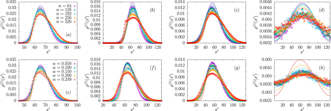
Figure 5. Evolution of normalized marginal distributions of x of the MC simulations (circles) and MF (lines) for different time steps (a,e) t=50, (b,f) t=250, (c,g) t=450, and (d,h) t=4950. Plots (a-d) show the influence of different values of n for α=0.15, whilst plots (e-h) show different α’s for a fixed n=192.

While both methods show reasonably good agreement in Figure 5, we find that the agreement can be further improved by optimizing β. Revisiting Figure 4d and extending our earlier analysis for m=1 to m=2, we observe that the critical value βc minimizing ΔS2̄ follows a power-law dependence, axb. For m=2, the fit yields a=3.3±0.11 and b=0.193±0.0065, contrasting with the linear behavior found for m=1. This indicates that increasing the model complexity (from m=1 to m=2) modifies the parameter dependence. However, no significant changes are observed beyond m=2 up to m=4, as seen in Figure 4D—a point we will address in detail later. Importantly, we note that lower-density cases do not provide the best agreement between the two methods, revealing non-trivial model-specific characteristics that lack complete theoretical understanding.

3.3 m=4 case

The last case we discuss in this work is the case with four species moving along the x and ydirections. More precisely, their initial distributions have mean value: μx(1)=l/4 and μy(1)=l/2, μx(2)=3l/4 and μy(2)=l/2, μx(3)=l/2 and μy(3)=l/4, and μx(4)=l/2 and μy(4)=3l/2 as we expected to be by our previous definition. Similarly, the static floor fields assume the form û(1)=ex, û(2)=ey, û(3)=ex, and û(4)=ey (see Equation 10). Similarly to the two prior cases, having an initial condition with radial symmetry about the lattice center, also makes the four species present a symmetric “cross section” of the distribution, i.e., the distribution on the direction perpendicular to û(q) shows no asymmetry. Thus, studying the marginal distribution of x of the species q=1 or q=3 would be no different from studying the marginal distribution of y of the species q=2 and q=4 given the system’s initial arrangement and static floor fields (see Figure 2).

With this in mind, Figure 6 displays the particle distribution ρ(1)(x) for different values of n using α=0.249 at four time points: (a) t=50, (b) t=250, (c) t=450, and (d) t=4950. Our analysis reveals two key observations:

Figure 6
Eight graphs display distributions of \(\rho(D)\) versus \(x'\). Panels (a) to (d) show varying \(n\) values (64, 128, 256, 320, 384), while panels (e) to (h) use \(\alpha\) values (0.100, 0.150, 0.200, 0.249). Each graph illustrates data points and curves of different colors for comparison.

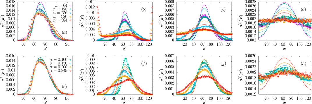
Figure 6. Evolution of normalized marginal distributions of x of the MC simulations (circles) and MF (lines) for different time steps (a,e) t=50, (b,f) t=250, (c,g) t=450, and (d,h) t=4950. Plots (a-d) show the influence of different values of n for α=0.249, whilst plots (e-h) show different α’s for a fixed n=256.

(1) First, the discrepancy between methods becomes more pronounced for larger n values in this regime of highly driven agents. Despite this disagreement, the MC simulations demonstrate the formation of transient condensates for n=320, as evidenced by the emerging peak at t=250.

(2) Second, the mean-field solution exhibits anomalous behavior at t=250, particularly in the left tail of ρ(1)(x), which appears bent near x100. Notably, however, both methods show qualitatively good agreement in the front tail of ρ(1)(x), suggesting synchronized drifting profiles in the steady state.

Building on our analysis of the m=4 case, Figure 6 presents the evolution of ρ(1)(x) distributions for various α values in a system with n=256 particles. We also examine the same four time points: (e) t=50, (f) t=250, (g) t=450, and (h) t=4950. The results reveal that while the wave fronts remain synchronized between MC simulations and mean-field theory, the MC distributions exhibit significantly greater dispersion. Returning to Figure 4d, we apply the same minimization procedure for ΔS2̄ used for the m = 1 and m = 2 cases. For m = 4, we obtain an excellent power-law fit identical in form to the m = 2 case, with fitted parameters a = 3.04 ± 0.23 and b = 0.176 ± 0.014.

It is important to note that, despite some differences in the evolution of particle profiles, a qualitatively similar behavior is observed in both cases when the systems are initialized with a normal distribution of particles in the environment. The interactions among particles—especially the interaction with counterflowing particles—tend to deform the initial distribution shape. Over time, however, after several rounds of confrontation and interaction, the particles begin to reorganize themselves, ultimately restoring a Gaussian-like behavior.

This transition from one Gaussian state to another is illustrated in Figure 7. In Figures 7a–e, we show the results from MC simulations, while Figure 7f corresponds to the mean field approximation. All plots refer to the case of m=4 species, n=256 particles, and interaction parameter α=0.249.

Figure 7
Graphs show Monte Carlo simulation data. Panels (a)-(e) illustrate density functions \(\rho(x)\) at different times \(t = 50, 150, 250, 450, 4850\) with normal fit (red line). Panel (f) shows \(R^2\) over time with Gaussian, transient, and mean-field annotations. Insets in (a) and (f) detail data fits.

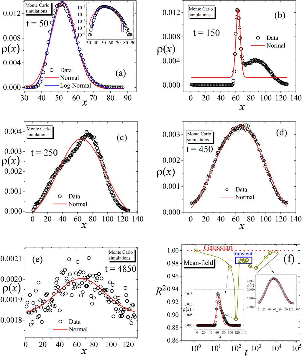
Figure 7. Plots (a–e) show the particle distribution at different times obtained via Monte Carlo simulations. At t=50, significant deviations from a normal distribution are observed. As time progresses, the system gradually returns to a Gaussian-like profile, culminating in a noisy steady-state distribution at t=400, as seen in plot (e). Plot (f) summarizes the corresponding results for the mean-field approximation. Here, the quality of the Gaussian fit over time is quantified by the coefficient of determination R2, represented by dark yellow circles. Initially, interactions among particles cause strong deviations, leading to a transient regime. At later times, the system converges again to a Gaussian distribution—less noisy than that of the Monte Carlo steady state. The inset in (a) compares normal and log-normal fits on a semi-logarithmic scale. The insets in (f) illustrate the particle profile at different stages of the evolution.

In Figure 7a, we observe the particle distribution at t=50. We observe that the initial Gaussian behavior is disrupted due to particle interactions. The red and blue curves represent normal and log-normal fits, respectively, with the latter providing a more accurate fit at this stage. The inset plot shows the same trend on a semi-log scale. By t=150, the distribution becomes strongly non-Gaussian, with a pronounced peak emerging, as shown in Figure 7b.

At t=250, the shape of the distribution becomes nearly triangular (Figure 7c), signaling the beginning of a return to Gaussianity. A good Gaussian fit is eventually recovered in Figure 7d, and a noisy but stable Gaussian distribution is observed at t=400, as shown in Figure 7e. This reflects the establishment of a steady state after extensive particles interactions.

Finally, in Figure 7f, we analyze the mean-field approximation. Unlike the MC simulations, which display the full evolution of the particle profile, we summarize the results using the coefficient of determination R2, which quantifies the quality of a normal distribution fit over time. These values are represented by circles. Initially, we observe a sharp decline in R2, indicating the breakdown of Gaussianity (illustrated in the inset). As t increases, the system goes through a transient (points inside blue rectangle) phase before recovering a Gaussian profile, again shown in the inset. This confirms that the same Gaussian-to-Gaussian behavior occurs in the mean-field scenario, in agreement with the MC simulations presented in Figures 7a–e.

4 Conclusion

In this work, we proposed a mean-field approximation to describe the dynamics of an agent-based model of m-species of particles. Specifically, we proposed a recurrence relation that shows the evolution of lattice gas dynamics with an asynchronous updating scheme in a Von Neumann neighborhood.

We showed that the MF method shows a good agreement with the particle dynamics implemented through MC simulation using initial conditions and static floor fields carrying polar symmetry in relation to the center of the lattice. We studied the cases of one, two, and four species, which, with the initial conditions, made for a sort of “controlled” environment so that we could access more easily the agreement between methods.

The MF approach carried a normalization constant exponent β, which relied on the parameters n and m, because the agreement of methods is strongly influenced by the complexity of the interactions. We showed that when one species is considered, its optimal value, βc, has a linear dependence on the total number of particles, when m=2 and m=4 it shows to be a function of some power of n.

We highlighted that our proposed mean-field approach is not bulletproof by showing what specific set of parameters made it show numerical instability due to competing terms inside the recurrence relation.

Despite studying only three cases, our approach is general enough to allow an arbitrary number of particles, even for initial conditions and/or species preferential directions of motion different from those studied in this work. Not only that, our framework proposed by Equation 3 presents a general feature of application to asynchronous lattice gas models, even reproducing the recurrence relation of other models such as the deterministic two-species dynamics studied in [21].

We are currently exploring higher systems with more than four species, which means that some species are going to present static floor field at angles lower than 90° with the x and ydirection. As a consequence, we expect to observe βc presenting a more complex dependency with n.

Finally, our model reveals a distinctive pattern we term the “Gaussian-to-Gaussian” transition. In this phenomenon, particles initially distributed in a Gaussian configuration undergo significant deformation of this pattern, only to eventually recover a Gaussian distribution after multiple interaction cycles. Both Monte Carlo simulations and mean-field theory reproduce this effect, though they follow different temporal evolution pathways.

Data availability statement

The original contributions presented in the study are included in the article/Supplementary Material, further inquiries can be directed to the corresponding author.

Author contributions

ES: Data curation, Writing – original draft, Supervision, Methodology, Investigation, Conceptualization, Software, Funding acquisition, Visualization, Writing – review and editing, Resources, Project administration, Validation, Formal Analysis. RD: Methodology, Formal Analysis, Conceptualization, Project administration, Validation, Visualization, Supervision, Writing – original draft, Funding acquisition, Software, Investigation, Resources, Data curation, Writing – review and editing. SG: Project administration, Formal Analysis, Data curation, Validation, Writing – review and editing, Writing – original draft, Resources, Conceptualization, Supervision, Visualization, Funding acquisition, Software, Investigation, Methodology.

Funding

The author(s) declare that financial support was received for the research and/or publication of this article. We gratefully acknowledge the partial support provided by CNPq: E. V. ES under grant 153315/2024-5, RS under grant 304575/2022-4, and SG under grant 314738/2021-5.

Acknowledgments

We appreciate the availability of computational resources from the Lovelace cluster at IF-UFRGS.

Conflict of interest

The authors declare that the research was conducted in the absence of any commercial or financial relationships that could be construed as a potential conflict of interest.

Generative AI statement

The author(s) declare that no Generative AI was used in the creation of this manuscript.

Publisher’s note

All claims expressed in this article are solely those of the authors and do not necessarily represent those of their affiliated organizations, or those of the publisher, the editors and the reviewers. Any product that may be evaluated in this article, or claim that may be made by its manufacturer, is not guaranteed or endorsed by the publisher.

Supplementary material

The Supplementary Material for this article can be found online at: https://www.frontiersin.org/articles/10.3389/fphy.2025.1648895/full#supplementary-material

References

1. Guo X, Angulo A, Tavakoli A, Robartes E, Chen TD, Heydarian A. Rethinking infrastructure design: evaluating pedestrians and vrus’ psychophysiological and behavioral responses to different roadway designs. Scientific Rep (2023) 13:4278. doi:10.1038/s41598-023-31041-9

PubMed Abstract | CrossRef Full Text | Google Scholar

2. Geoerg P, Schumann J, Boltes M, Kinateder M. How people with disabilities influence crowd dynamics of pedestrian movement through bottlenecks. Scientific Rep (2022) 12:14273. doi:10.1038/s41598-022-18142-7

PubMed Abstract | CrossRef Full Text | Google Scholar

3. Nicholls VI, Wiener J, Meso AI, Miellet S. The impact of perceptual complexity on road crossing decisions in younger and older adults. Scientific Rep (2024) 14:479. doi:10.1038/s41598-023-49456-9

PubMed Abstract | CrossRef Full Text | Google Scholar

4. Zhang H, Xu J, Jia L, Shi Y. Modelling the walking behavior of pedestrians in the junction with chamfer zone of subway station. Physica A: Stat Mech its Appl (2022) 602:127656. doi:10.1016/j.physa.2022.127656

CrossRef Full Text | Google Scholar

5. Huang D, Yang Y, Peng X, Huang J, Mo P, Liu Z, et al. Modelling the pedestrian’s willingness to walk on the subway platform: a novel approach to analyze in-vehicle crowd congestion. Transportation Res E: Logistics Transportation Rev (2024) 181:103359. doi:10.1016/j.tre.2023.103359

CrossRef Full Text | Google Scholar

6. Stock EV, da Silva R. Lattice gas model to describe a nightclub dynamics. Chaos, Solitons and Fractals (2023) 168:113117. doi:10.1016/j.chaos.2023.113117

CrossRef Full Text | Google Scholar

7. Stock EV, da Silva R, Gonçalves S. Nightclub bar dynamics: statistics of serving times. The Eur Phys J B (2024) 97:179. doi:10.1140/epjb/s10051-024-00803-3

CrossRef Full Text | Google Scholar

8. Stock EV, da Silva R. Exploring crossing times and congestion patterns at scramble intersections in pedestrian dynamics models: a statistical analysis. Physica A: Stat Mech its Appl (2024) 649:129942. doi:10.1016/j.physa.2024.129942

CrossRef Full Text | Google Scholar

9. Vissers T, van Blaaderen A, Imhof A. Band formation in mixtures of oppositely charged colloids driven by an ac electric field. Phys Rev Lett (2011) 106:228303. doi:10.1103/PhysRevLett.106.228303

PubMed Abstract | CrossRef Full Text | Google Scholar

10. Stock EV, da Silva R, Fernandes HA. Statistics, distillation, and ordering emergence in a two-dimensional stochastic model of particles in counterflowing streams. Phys Rev E (2017) 96:012155. doi:10.1103/PhysRevE.96.012155

PubMed Abstract | CrossRef Full Text | Google Scholar

11. Zhang J, Seyfried A. Comparison of intersecting pedestrian flows based on experiments. Physica A: Stat Mech its Appl (2014) 405:316–25. doi:10.1016/j.physa.2014.03.004

CrossRef Full Text | Google Scholar

12. Helbing D, Farkas I, Vicsek T. Simulating dynamical features of escape panic. Nature (2000) 407:487–90. doi:10.1038/35035023

PubMed Abstract | CrossRef Full Text | Google Scholar

13. Majumdar SN, Evans MR, Zia RKP. Nature of the condensate in mass transport models. Phys Rev Lett (2005) 94:180601. doi:10.1103/physrevlett.94.180601

PubMed Abstract | CrossRef Full Text | Google Scholar

14. Katz S, Lebowitz JL, Spohn H. Phase transitions in stationary nonequilibrium states of model lattice systems. Phys Rev B (1983) 28:1655–8. doi:10.1103/PhysRevB.28.1655

CrossRef Full Text | Google Scholar

15. Helbing D, Molnár P. Social force model for pedestrian dynamics. Phys Rev E (1995) 51:4282–6. doi:10.1103/PhysRevE.51.4282

PubMed Abstract | CrossRef Full Text | Google Scholar

16. Oliveira CLN, Vieira AP, Helbing D, Andrade JS, Herrmann HJ. Keep-left behavior induced by asymmetrically profiled walls. Phys Rev X (2016) 6:011003. doi:10.1103/PhysRevX.6.011003

CrossRef Full Text | Google Scholar

17. Kleintjens L, Van der Haegen R, van Opstal L, Koningsveld R. Mean-field lattice-gas modelling of supercritical phase behavior. The J Supercrit Fluids (1988) 1:23–30. doi:10.1016/0896-8446(88)90006-X

CrossRef Full Text | Google Scholar

18. Bernard MO, Plapp M, Jfmc G. Mean-field kinetic lattice gas model of electrochemical cells. Phys Rev E (2003) 68:011604. doi:10.1103/PhysRevE.68.011604

CrossRef Full Text | Google Scholar

19. Dickman R. Mean-field theory of the driven diffusive lattice gas. Phys Rev A (1988) 38:2588–93. doi:10.1103/physreva.38.2588

PubMed Abstract | CrossRef Full Text | Google Scholar

20. da Silva R, Hentz A, Alves A. Stochastic model of self-driven two-species objects inspired by particular aspects of a pedestrian dynamics. Physica A: Stat Mech its Appl (2015) 437:139–48. doi:10.1016/j.physa.2015.05.104

CrossRef Full Text | Google Scholar

21. Cividini J, Hilhorst HJ, Appert-Rolland C. Crossing pedestrian traffic flows, the diagonal stripe pattern, and the chevron effect. J Phys A: Math Theor (2013) 46:345002. doi:10.1088/1751-8113/46/34/345002

CrossRef Full Text | Google Scholar

22. Appert-Rolland C, Cividini J, Hilhorst H, Degond P. Pedestrian flows: from individuals to crowds. Transportation Res Proced (2014) 2:468–76. doi:10.1016/j.trpro.2014.09.062

CrossRef Full Text | Google Scholar

23. Stock EV, da Silva R. Coexistence and crossover phenomena in a fermi-like model of particles in counterflowing streams. Phys Rev E (2020) 102:022139. doi:10.1103/PhysRevE.102.022139

PubMed Abstract | CrossRef Full Text | Google Scholar

24. Schadschneider A, Chraibi M, Seyfried A, Tordeux A, Zhang J. Pedestrian dynamics: from empirical results to modeling. Cham: Springer International Publishing (2018). p. 63–102. doi:10.1007/978-3-030-05129-7_4

CrossRef Full Text | Google Scholar

25. Press WH, Sa T, Vetterling WT, Flannery BP. Numerical recipes in fortran 77: the art of scientific computing. vol. 1 (1996).

Google Scholar

26. Giddings JC, Byring H. A molecular dynamic theory of chromatography. The J Phys Chem (1955) 59:416–21. doi:10.1021/j150527a009

CrossRef Full Text | Google Scholar

27. da Silva R, Lamb LC, Lima EC, Dupont J. A simple combinatorial method to describe particle retention time in random media with applications in chromatography. Physica A: Stat Mech its Appl (2012) 391:1–7. doi:10.1016/j.physa.2011.08.006

CrossRef Full Text | Google Scholar

28. Stock EV, da Silva R, da Cunha CR. Numerical study of condensation in a fermi-like model of counterflowing particles via gini coefficient. J Stat Mech Theor Exp (2019) 2019:083208. doi:10.1088/1742-5468/ab333d

CrossRef Full Text | Google Scholar

29. da Silva R, Stock EV. Mobile-to-clogging transition in a fermi-like model of counterflowing particles. Phys Rev E (2019) 99:042148. doi:10.1103/PhysRevE.99.042148

PubMed Abstract | CrossRef Full Text | Google Scholar

Keywords: pedestrian dynamics, mean-field, transport equation, lattice gas, stochastic process, multi-species

Citation: Stock EV, Da Silva R and Gonçalves S (2025) Mean-field and Monte Carlo analysis of multi-species agent dynamics. Front. Phys. 13:1648895. doi: 10.3389/fphy.2025.1648895

Received: 17 June 2025; Accepted: 29 July 2025;
Published: 26 August 2025.

Edited by:

Ryosuke Yano, Tokio Marine dR Co., Ltd., Japan

Reviewed by:

Giovanni Modanese, Free University of Bozen-Bolzano, Italy
Jan Haskovec, BESE Division, Saudi Arabia., Saudi Arabia

Copyright © 2025 Stock, Da Silva and Gonçalves. This is an open-access article distributed under the terms of the Creative Commons Attribution License (CC BY). The use, distribution or reproduction in other forums is permitted, provided the original author(s) and the copyright owner(s) are credited and that the original publication in this journal is cited, in accordance with accepted academic practice. No use, distribution or reproduction is permitted which does not comply with these terms.

*Correspondence: Roberto da Silva, cmRhc2lsdmFAaWYudWZyZ3MuYnI=

Disclaimer: All claims expressed in this article are solely those of the authors and do not necessarily represent those of their affiliated organizations, or those of the publisher, the editors and the reviewers. Any product that may be evaluated in this article or claim that may be made by its manufacturer is not guaranteed or endorsed by the publisher.