Improved daily tourism demand prediction model based on deep learning approach

The rapid escalation in tourist visitation poses significant challenges, including traffic congestion, overcapacity at scenic attractions, heightened risks of safety incidents, and diminished visitor satisfaction. To optimize scenic area management through better resource allocation and service delivery, as well as to facilitate informed travel and visitor planning, this study proposes a hybrid predictive model, called Secretary Bird Optimization Algorithm-Convolutional Neural Network-Bidirectional Gated Recurrent Unit-Attention Model (SBOA-CBAM), for forecasting tourist volume within scenic areas. The methodology involves constructing a foundational Convolutional Neural Network-Bidirectional Gated Recurrent Unit-Attention Mechanism (CBA) model, where input data pre-processed via the Maximal Information Coefficient (MIC) algorithm undergoes feature extraction using Convolutional Neural Network (CNN), followed by bidirectional temporal feature mining via BiGRU, and output weighting via an Attention Mechanism to emphasize critical features and generate predictions. Subsequently, the Secretary Bird Optimization Algorithm (SBOA) is employed to autonomously identify the optimal hyperparameter configuration for the CBA model, thereby enhancing its predictive accuracy and computational efficiency. Comparative simulation experiments demonstrate the high applicability of the CBA model for scenic area tourist flow forecasting and reveal that the SBOA-optimized CBAM model achieves statistically significant performance enhancements, namely, a 3.8966% increase in R², alongside reductions of 19.9025% in RMSE, 12.1726% in MAE, 8.3196% in MAPE, and 43.7662% in MSE. Statistical validation via the Wilcoxon signed-rank test confirmed the significance of the improvements (RMSE: p = 0.0001; MAE: p = 0.0007), with substantial effect sizes indicated by Cohen’s d values of 0.8982 (RMSE) and 0.7028 (MAE). These findings corroborate that the SBOA algorithm not only substantially elevates predictive precision but also enhances model stability and robustness against disturbances.

1 Introduction

Over the past few decades, China’s tourism sector has undergone exponential expansion. Concurrently, evolving societal attitudes and lifestyle transformations have substantially heightened travel frequency and extended durations [1]. While this growth has served as a catalyst for economic prosperity and stimulated development in ancillary sectors, it has also introduced unforeseen operational risks. The unprecedented surge in tourist volumes elevates accident probability and exacerbates managerial complexities at destination sites. Therefore, accurate forecasting of tourist flows has become imperative for optimizing tourism service quality through strategic resource allocation and proactive management frameworks.

In recent years, artificial intelligence techniques including, Support Vector Machines, LSTM networks, Bidirectional Long short-term memory (LSTM) networks, and improved models developed by various researchers have been increasingly employed in predictive research [2]. The research team led by Ni developed a multilayer neural network model termed Spatial Principal Component Analysis-CNN-LSTM to predict daily tourist flows [1], Chen and colleagues proposed a hybrid CNN-Bidirectional LSTM prediction methodology for tourism demand forecasting, integrating the Boruta algorithm, Bidirectional LSTM, and CNN [3]. Li’s research group proposed a novel visitor volume prediction approach utilizing the K-means algorithm, Particle Swarm Optimization, and Quadratic Support Vector Machines [4]. Additionally, Qin’s team introduced the CNN-Improved Quantum-inspired Reinforcement Learning LSTM tourist flow prediction model [5], Meng and Dou developed an Empirical Mode Decomposition-CNN-LSTM short-term forecasting framework for railway passenger traffic, incorporating empirical mode decomposition, CNN, and LSTM models [6]. Constantino’s research team simulated and predicted tourist flows in Mozambique through an Artificial Neural Network model, demonstrating superior predictive performance of artificial neural networks [7]. Wang and Liu proposed a novel multi-factor hybrid integrated learning method designated Improved Complete Ensemble Empirical Mode Decomposition with Adaptive Noise-Levy Flight Black Swan Algorithm, combining Improved Complete Ensemble Empirical Mode Decomposition with Adaptive Noise, Least Absolute Shrinkage and Selection Operator, Autoregressive Integrated Moving Average, Support Vector Regression, and BiGRU for tourism demand prediction [8]. While, Lu’s research group implemented the CNN-LSTM model for daily tourist flow forecasting in scenic areas, employing genetic algorithms to optimize neuron configuration within the model [9]. Li and collaborators presented a Particle Swarm Optimization-Least Squares Support Vector Machine method for forecasting tourism volumes in scenic spots [4]. Gao’s team developed a Hybrid Neural Network model for scenic spot passenger flow prediction, integrating CNN and LSTM as CNN-LSTM [10]. Chen’s research group constructed a tourism traffic prediction framework combining Boruta, Bidirectional LSTM, and CNN [3]. Then, Gu’s team utilized a spatiotemporal CNN model to capture spatio-temporal dependencies in tourist traffic patterns [11].

Nevertheless, LSTM networks exhibit limitations, including structural complexity, excessive parameterization, slow convergence rates, and prolonged training times [12]. To address these constraints, Cho and colleagues developed the GRU, which features a simplified architecture and enhanced training efficiency compared to LSTM [13, 14]. As a result, GRU has gained widespread application in short-term traffic flow forecasting [15], travel time prediction [15], and highway speed estimation [16]. Meanwhile, Ren’s research team employed a One-Dimensional CNN to extract local traffic flow features, complemented by Recurrent Neural Network variants (including LSTM and GRU) to capture long-term trend characteristics [17]. When, Yang’s group established in 2022 a hybrid CNN-GRU model for traffic volume prediction, where spatial information is processed through CNN while long-term sequential dependencies are captured via GRU [18]. As for, Yuan’s research team, they integrated CNN and GRU to construct a unified prediction model designed for enhanced accuracy in traffic time series forecasting [19].

The unidirectional GRU architecture exhibits constrained capacity for comprehensive sequential information extraction relative to the BiGRU configuration. The Attention Mechanism replicates the selective information processing paradigm observed in human visual cognition. Neurological systems inherently filter non-essential stimuli, transforming high-dimensional sensory data into focused perceptual subsets. This biological process facilitates efficient extraction of salient features from attended information segments to optimize response efficiency [12, 20, 21]. Multiple research teams have developed predictive frameworks integrating these computational architectures. For example, Ren and colleagues developed a hybrid prediction model for power load forecasting that integrates CNN, BiGRU, and Attention Mechanism components [22], Na’s research group proposed a combined modeling architecture for time-series data prediction incorporating CNN, BiGRU, and Attention Mechanism modules [23], Niu’s research team established a hybrid modeling framework for multi-energy load forecasting through integration of CNN, BiGRU, and Attention Mechanism methodologies [24], Chai and collaborators engineered a traffic flow forecasting system featuring CNN-based feature extraction from traffic flow data, with BiGRU-Attention Mechanism modules processing daily and weekly temporal traffic patterns [20]. With, Chen’s research group put forward an improved CBA model. This model was based on an enhanced Sparrow Search Algorithm, aiming to boost the model’s robustness and accuracy in the assessment of lithium-battery health status [25], Dai and his colleague presented an enhanced variant of the whale optimization algorithm is employed to optimize the hyperparameters in the CBA model, leading to an elevation in the accuracy of predictions [2]. Sun’s research group employed the WOA algorithm to fine-tune the hyper-parameters of the CBA model, this, in turn, brought about an increase in the accuracy of satellite clock bias prediction [26]. Wu and his team proposed a new prediction that fused the Snow Ablation Optimization (SAO),CNN,BiGRU and Attention for position prediction for space teleoperation, the SAO algorithm is introduced into the hyper-parameter selection to solve the problem that the custom selection way of hyper-parameter obviously cannot guarantee optimality [27], and Yuan and his team proposed an improved CBA model, which is based on the Northern Grey Wolf Optimization Algorithm (NGO), for electricity load forecasting. The NGO is employed to fine-tune the hyperparameters of the BiGRU model [28].

With the advent of the Internet era, an increasing number of netizens obtain information through clients such as computers and mobile phones, using internet search engines to look for the things they are interested in/or the needs they have. The changes in the search volume of relevant information over a period of time can indirectly reflect the future behavioral characteristics of the events being concerned about. Therefore, scholars have incorporated internet search information into the prediction model. Duan and his team combined the network search index with the GWO-LightGBM- CEEMDAN model to develop a prediction model for the proportion of influenza-like illnesses (ILI). The findings indicated that the inclusion of the network search index enhanced the model’s prediction accuracy [29]. Zhou et al investigated the impact of the network search index on the early warning and prediction of COVID-19 epidemic trends [30]. Guo et al merged the network search index with the LSTM (LSTM) model to construct a predictive model specifically designed for estimating the incidence rate of hepatitis E. The results of this study highlighted a subtle yet discernible correlation between the network search index and the incidence of hepatitis E. Moreover, the trends exhibited by the network search index were found to be largely congruent with those of the hepatitis E incidence, suggesting a potential utility of the network search index as an auxiliary tool for monitoring and predicting the epidemiological patterns of hepatitis E [31]. Dong et al proposed a GMM-CEEMD-SGIA-LSTM hybrid carbon dioxide emission prediction model based on search engine keyword search and carbon dioxide emission data, with the search engine keyword search data having a strong correlation with CO₂ emissions [32].

Tourists collect information such as accommodation, transportation, weather, and travel guides through the internet before traveling [33]. The massive data generated when tourists use search engines is an objective reflection of their potential travel demands [34] and a representation of their travel intentions [35], featuring immediacy, predictability, and high accessibility.

The CNN-BiGRU-Attention Mechanism (CBA) model demonstrates efficacy in time-series forecasting. Recognizing that Internet Search Index (ISI) data can reflect potential tourist travel intent, this study proposes a CBA model incorporating ISI to predict scenic spot tourist flow. The Maximal Information Coefficient (MIC) algorithm is employed to screen highly relevant features, including ISI-derived attributes. To enhance prediction accuracy, this research integrates the Secretary Bird Optimization Algorithm (SBOA) with CNN, BiGRU, and AM to construct a hybrid predictive model, designated SBOA-CBAM. This model utilizes MIC-filtered tourist flow and ISI data as input. The input data undergoes feature vector extraction via CNN, followed by bidirectional temporal sequence processing through BiGRU to capture latent data characteristics. An attention mechanism subsequently weights the BiGRU output states, emphasizing critical tourist flow features to generate the final predictions. The SBOA algorithm is applied to autonomously optimize the hyperparameters of the CBA architecture, thereby augmenting its fitting capability and predictive accuracy. Experimental results demonstrate that the SBOA-CBAM model achieves statistically superior performance in prediction accuracy compared to the baseline CBA model.

1.1 Research contributions

This study presents the following main contributions:

• Integration of Search Index Data with Feature Selection: Internet search index data, recognized as an indicator of potential travel intent, is incorporated into the tourist flow prediction data set. The Maximal Information Coefficient (MIC) algorithm is employed to rigorously screen and retain only the most relevant features, including those derived from the search index.

• Novel Hybrid Forecasting Architecture: A novel hybrid architecture integrating Convolutional Neural Networks (CNN), Bidirectional Gated Recurrent Units (BiGRU), and an Attention Mechanism (AM), termed the CNN-BiGRU-Attention (CBA) model, is proposed specifically for scenic spots tourist flow forecasting.

• Hyperparameter Optimization via Metaheuristics: The Secretary Bird Optimization Algorithm (SBOA) is leveraged to autonomously optimize the hyperparameters of the proposed CBA model, thereby enhancing its predictive accuracy and generalization capability.

• Empirical Validation and Comparative Analysis: The effectiveness of the resulting SBOA-CNN-BiGRU-Attention (SBOA-CBAM) model is rigorously validated using tourist flow data from the Jiuzhaigou Scenic Area spanning 1 January 2013 to 31 July 2017. Comprehensive comparative experiments demonstrate its superior performance over established baseline models, including the CBA model itself, Backpropagation Neural Networks (BP), Support Vector Machines (SVM) and Extreme Learning Machines (ELM).

1.2 Organization

The remainder of this paper is structured as follows: Section 2 delineates the theoretical foundations and algorithmic workflow of the Secretary Bird Optimization Algorithm (SBOA), while the Section 3 elaborates on the formulation and implementation procedures of the proposed SBOA-CBAM (Secretary Bird Optimization Algorithm-Convolutional Neural Network-Bidirectional Gated Recurrent Unit-Attention Mechanism) modeling framework. Section 4 empirically validates the predictive performance of the SBOA-CBAM model. Finally, Sections 5, 6 present the concluding remarks and policy implications.

2 Secretary bird optimization algorithm

The Secretary Bird Optimization Algorithm (SBOA), proposed by Fu in 2024, is a swarm intelligence-based metaheuristic. The algorithm’s optimization process comprises three distinct phases which are as follows; an initialization phase, a prey hunting phase (exploration), and a predator evasion phase (exploitation). Details are shown as below [36, 37].

2.1 Initial preparation phase

During the early stages of SBOA deployment, the initialization of the search domain for the Secretary bird algorithm is implemented using Equation 1.

$X_{i,j}=l{b}_j+r\times \left(u{b}_j-l{b}_j\right),i=1,2,\dots ,N,j=1,2,\dots ,\mathit{Dim}(1)$

where X_i,j, lb_j, and ub_j are symbols for denoting the ith secretary bird’s position, along with its upper and lower limits, respectively; and the variable r is a random number between 0 and 1.

SBOA is a population-based method that is initially used to optimize the number of candidate solutions through Equation 2. Each iteration generates a random candidate solution X within the problem’s interval. The current optimal solution is approximated as the optimal solution of each iteration.

$X={\left[\begin{array}{cccccc}{X}_{1,1}& X_{1,2}& \cdots & X_{1,j}& \cdots & X_{1,\mathit{Dim}}\\ X_{2,1}& X_{2,2}& \cdots & X_{2,j}& \cdots & X_{2,\mathit{Dim}}\\ ⋮& ⋮& \ddots & ⋮& \ddots & ⋮\\ X_{i,1}& X_{i,2}& \cdots & X_{i,j}& \cdots & X_{i,\mathit{Dim}}\\ ⋮& ⋮& \ddots & ⋮& \ddots & ⋮\\ X_{N,1}& X_{N,2}& \cdots & X_{N,j}& \cdots & X_{N,\mathit{Dim}}\end{array}\right]}_{N\times \mathit{Dim}}(2)$

Every single secretary bird denotes a possible answer to an optimization problem. Consequently, the objective function for which it can be calculated relied on the values of the variables obtained from each secretary bird. On this basis, Equation 3 is employed to turn the resulting objective function value into a vector.

$F={\left[\begin{array}{l}{F}_1\\ ⋮\\ F_2\\ ⋮\\ F_N\end{array}\right]}_{N\times 1}={\left[\begin{array}{l}f\left(X_1\right)\\ ⋮\\ f\left(X_2\right)\\ ⋮\\ f\left(X_N\right)\end{array}\right]}_{N\times 1}(3)$

Here, the objective function values of secretary birds are denoted by the vector F, with F_i representing the value of the ith bird’s objective function. Evaluating the quality of a candidate solution involves comparing these objective function values to determine the best solution for a particular problem. In the course of each iteration, the positions of the secretary birds and the values of the objective function undergo updates. It is therefore crucial to continuously identify the optimal candidate solution at each step. This iterative process ensures that the final solution chosen is the most effective for solving the problem at hand.

2.2 Secretary birds’ strategies of hunting for prey (exploration phase)

Secretary birds undergo three distinct stages when hunting snakes: locating their prey, depleting the prey’s energy, and then attacking. The hunting process of secretary birds are evenly divided, with each stage occupying an equal time interval, each corresponding to one of the following bird’s hunting stages: locating, depleting, and attacking prey.

2.2.1 Stage 1 (prey locating, $t<\frac{1}{3}T$)

Secretary birds initiate their hunt by seeking out likely prey, such as snakes. Their exceptionally sharp vision allows them to detect snakes concealed within the high grasses of the savannah swiftly.

Consequently, the secretary bird’s positional updates method in the prey-searching stage is modeled using the Equations 4, 5:

$x_{i,j}^{\text{newP}1}=x_{i,j}+\left(x_{{\text{random}}_1}-x_{{\text{random}}_2}\right)\times R1(4)$

$X_i=\left\{\begin{array}{l}{X}_i^{\text{new},\mathrm{P}1},\text{if}{F}_i^{\text{new},\mathrm{P}1}<F_i\\ X_i,\text{else}\end{array}\right.(5)$

where t signifies the current iteration count; T indicates the maximum limit of iterations; $X_i^{\text{new},\mathrm{P}1}$ refers to the new condition of the ith secretary bird in the early stage; xrandom1 and xrandom2 are the random candidate solutions for the initial phase iteration; R1 denotes an array that is randomly generated with dimensions (1 × Dim), ranging from 0 to 1; Dim refers to the solution space’s dimension; $X_{i,j}^{\text{new},\mathrm{P}1}$ signifies the value of its jth dimension; $F_i^{\text{new},\mathrm{P}1}$ signifies the fitness value of its goal.

2.2.2 Stage 2 (prey consuming, $\frac{1}{3}T<t<\frac{2}{3}T$)

When the secretary bird spots the snake, it will adopt a special hunting method. Unlike other birds that will immediately attack prey, the secretary bird often relies on its nimble footwork to navigate around serpents. The secretary bird stands still, watching the snake’s every move from above based on its sharp perception analyzing the snake’s movements. The secretary bird hovers, jumps, and gradually irritates the snake to consume the snake’s patience and power. In this phase, Brownian motion (RB) is applicable for simulating the stochastic movement of the secretary bird via Equations 6, 7.

$x_{i,j}^{\text{newP}1}=x_{\text{best}}+\mathit{exp}\left({\left(t/T\right)}^{\wedge }4\right)\times \left(RB-0.5\right)\times \left(x_{\text{best}}-x_{i,j}\right)(6)$

$X_i=\left\{\begin{array}{l}{X}_i^{\text{new},\mathrm{P}1},\text{if\hspace{0.17em}}{F}_i^{\text{new},\mathrm{P}1}<F_i\\ X_i,\text{else}\end{array}\right.(7)$

where, $\text{RB}=\text{randn}\left(1,\mathrm{Dim}\right)$,1×Dim Random arrays are generated using randn (1, Dim) following the standard normal distribution, with xbest is the current optimal value.

2.2.3 Stage 3 (prey attacking, $t>\frac{2}{3}T$)

Upon the snake’s exhaustion, the secretary bird discerns the opportune moment, expeditiously engages its powerful leg muscles, and launches an offensive against the snake. For this reason, the secretary bird uses the following partition described in Equations 8–12 to update its position during this.

$x_{i,j}^{\text{newP}1}=x_{\text{best}}+\left(\left(1-\frac{t}{T}\right)\wedge \left(2\times \frac{t}{T}\right)\right)\times x_{i,j}\times RL(8)$

$X_i=\left\{\begin{array}{l}{X}_i^{\text{new},\mathrm{P}1},\text{if\hspace{0.17em}}{F}_i^{\text{new},\mathrm{P}1}<F_i\\ X_i,\text{else}\end{array}\right.(9)$

The use of weighted Levy flight, known as RL, improves the accuracy of optimization processes. This method enhances precision by allowing for more efficient exploration of potential solutions in the optimization process.

$RL=0.5\times Levy\left(\mathit{Dim}\right)(10)$

Here is the function expression provided for Levy (Dim):

$Levy\left(D\right)=s\times \frac{\upsilon \times \sigma }{{\left|\nu \right|}^{\frac{1}{\eta }}}(11)$

The equation involves fixed value s = 0.01 and n = 1.5. Random variables U,V fall between 0 and 1. The symbol σ is determined by a specific calculation process.

$\sigma ={\left(\frac{\mathrm{\Gamma }\left(1+\eta \right)\times \sin \left(\frac{\pi \eta }{2}\right)}{\mathrm{\Gamma }\left(\frac{1+\eta }{2}\right)\times \eta \times 2\left(\frac{\eta -1}{2}\right)}\right)}^{1/\eta }(12)$

In this equation, the symbol $\mathrm{\Gamma }$ denotes the gamma function and the parameter $\eta$ is equal to 1.5

2.3 Secretary birds’ strategies of escaping from predators (exploitation phase)

The secretary bird’s natural enemies are large predators. The first strategy of escaping from predators is to run away or run fast, while the second strategy is camouflage, making them harder for predators to spot them.

The first strategy is modeled by the Equation 13.

$X_{i,j}^{\text{new},\mathrm{P}2}=\left\{\begin{array}{l}{C}_1:x_{\text{best}}+\left(2\times RB-1\right)\times {\left(1-\frac{t}{T}\right)}^2\times x_{i,j},\text{if}rand<r_i\\ C_2:x_{i,j}+R_2\times \left(x_{\text{random}}-K\times x_{i,j}\right),\text{else}\end{array}\right.(13)$

Equation 14 expresses the second strategy.

$X_i=\left\{\begin{array}{l}{X}_i^{\text{new},\mathrm{P}2},\text{if\hspace{0.17em}}{F}_i^{\text{new},\mathrm{P}2}<F_i\\ X_i,\text{else}\end{array}\right.(14)$

where, C₁ denotes the strategy of environmental camouflage; C₂ represents the strategy of flying or running away; r = 0.5; R₂ represents the randomly-generated array which has the dimension (1×Dim) and obeys the normal distribution, xrandom represents the random chosen solution.

Random integer 1 or 2 represented by K, calculated as follows Equation 15:

$K=round\left(1+rand\left(1,1\right)\right)(15)$

2.4 SBOA workflow

The workflow chart of SBOA is shown in Figure 1.

Figure 1

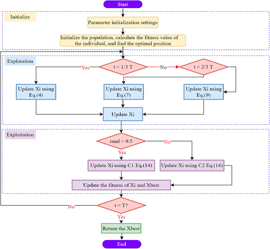
Figure 1. The SBOA workflow.

2.5 Feasibility analysis of the selected algorithms

The CEC2017 typical function set contains 29 functions, covering unimodal, simple multimodal, hybrid, and composite functions, and is commonly used to evaluate the performance of optimization algorithms. To verify the feasibility of selecting the SBOA algorithm, this paper selects 10 typical functions from it for testing. Among them, unimodal functions F1 and F3 are chosen to test the convergence ability of the algorithm, simple multimodal functions F4 and F7 are selected to examine the ability to jump out of local optima, hybrid functions F12 and F15 are picked to assess the capability of handling complex combined functions, and composite functions F22, F25, F28, and F30 are selected to test the optimization ability in highly complex scenarios. Meanwhile, comparisons are made with the Hiking Optimization Algorithm (HOA) [38], Harris Hawks Optimization (HHO) [39], Whale Optimization Algorithm (WOA) [40], Particle Swarm Optimization (PSO) [41] and Genetic Algorithm (GA) [42]. The population size is set to 30, the number of iterations is 1,000, and the number of runs is 30. Figures 2–4 show the average convergence curves, box plots, effect radar charts, and bar charts of the 5 algorithms when optimizing the above 10 functions.

Figure 2

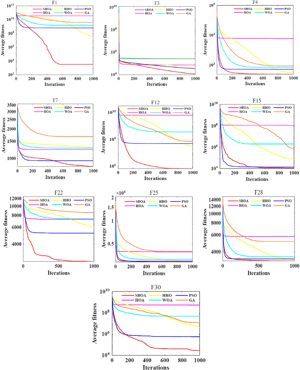
Figure 2. Average convergence curves of different algorithms.

Figure 3

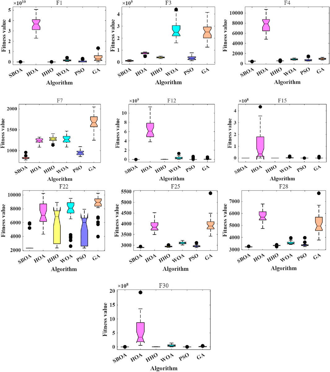
Figure 3. Box plots of different algorithms.

Figure 4

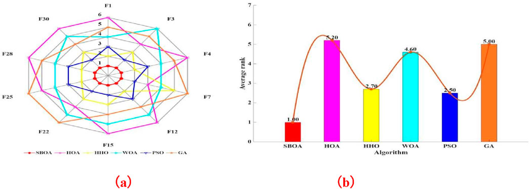
Figure 4. Radar charts and bar charts of optimization effects of different algorithms. (a) Radar charts (b) bar charts.

As can be seen from Figures 2–4, when the five algorithms including SBOA, HOA, HHO, WOA, PSO, and GA are used to optimize 10 functions such as F1, F3, F4, F7, F12, F15, F22, F25, F28, and F30, SBOA shows better and more stable optimization performance.

3 SBOA-CNN-Bigru-attention model

3.1 Convolutional neural networks (CNN)

A Convolutional Neural Network (CNN) constitutes a specific variety of feedforward neural network. It is characterized by convolutional computations and a deep-layered architecture. CNNs extract local features of the input data through convolutions and generate complex feature representations via multi-layer convolutions and pooling. The key components of a CNN include the input layer, convolutional layer, pooling layer, and fully connected layer, as illustrated in Figure 5. The input layer is mainly responsible for receiving the initial samples. Meanwhile, the convolutional and pooling layers play vital roles in dimensionality reduction and feature extraction [43–45].

Figure 5

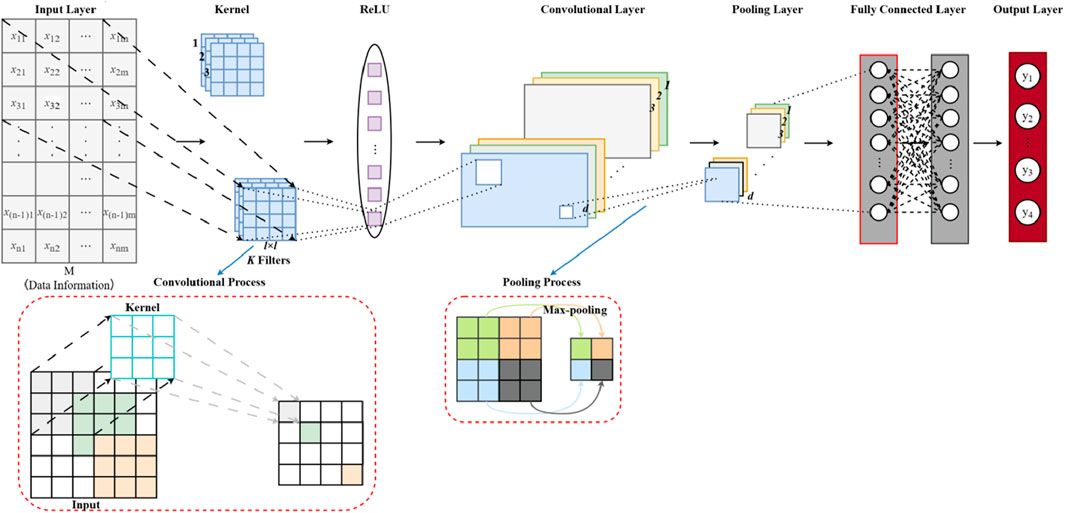
Figure 5. Basic structure of CNN_S.

3.1.1 Convolution layer

The convolution layer is responsible for the extraction of local features from input data via the process of convolution. Each convolution kernel within the convolution layer is capable of extracting a specific feature, and multiple convolution kernels can operate in parallel to extract a variety of features. The product operation is verified by the following Equation 16 [2, 46, 47].

$x_{i^{l+1},j^{l+1}}^{l+1}={\displaystyle \sum _{i=0}^H}{\displaystyle \sum _{i=0}^W}{\omega }_{i,j}\times {{x_{{i^l}^{+i}}^l}_{,}}_{j^{l+j}}(16)$

where, ${\omega }_{i,j}$ denotes the weights derived from the convolution kernel. $i^{l+i},j^{l+j}$ represents the position coordinates of the result of the convolution operation. For the processing to be precise, these coordinates have to meet the subsequent Equation 17 [2, 46, 47].

$\begin{array}{l}0⩽i^{l+1}<H^l-H+1\\ 0⩽j^{l+1}<W^l-W+1\end{array}(17)$

3.1.2 Pooling layer

The pooling layer constitutes an essential and fundamental element within the framework of deep-learning neural networks. It serves as a crucial architectural component that contributes significantly to the overall functionality and performance of these networks. Frequently employed to shrink the spatial dimensions of the initial sample, decrease the computational complexity, mitigate overfitting and extract key features from the initial sample. Consequently, it leads to a decreased parameter count and enhanced computational efficiency. Crucial pooling operations, including average pooling and max-pooling, assume central and indispensable functions in this procedure [2, 46, 47]. The pooling Layer is expressed as Equations 18, 19:

$x_{i^{l+1},j^{l+1}}^{l+1}=\frac{1}{HW}{\displaystyle \sum _{i=0}^H}{\displaystyle \sum _{j=0}^W}{x}_{i^l}^l\times H+i,j^l\times W=j(18)$

$x_{i^{l+1},j^{l+1}}^{l+1}=\underset{i<H,0⩽j<W}{\max }{x}_{i^l}^l\times H+i,j^l\times W+j(19)$

3.1.3 Fully-connected layer

The fully-connected layer combines the features that have been extracted from the previous layer, enabling it to carry out subsequent tasks like classification or regression. Every neuron in this layer forms connections with every single neuron in the layer that comes before it [2, 46, 47], and modeled as Equation 20:

$x^{l+1}=f\left(w{x}^l+b\right)(20)$

where, the $f$, $w$ , $b$ denotes the activation function, along with the matrix of weights and the matrix of biases.

3.2 Bidirectional gated recurrent unit (BiGRU)

The BiGRU model introduces a bidirectional structure to the GRU model to better capture the bidirectional dependency of sequence data. Comprising two separate GRU units, one for processing forward time series data and the other in a backward time series. The BiGRU model develops a full and in-depth understanding of the sequence. This particular architecture facilitates the model’s ability to incorporate both the prior and subsequent information of the data, thus facilitating better pattern recognition and prediction accuracy. Additionally, the BiGRU model incorporates key components such as reset gate, update gate, and a new candidate state, which together contribute to its superior performance in modeling sequential data [48, 49].

3.2.1 Reset gate

The Reset Gate is expressed as Equation 21 [50]:

$r_t=\sigma \left(W_r·\left[h_{t-1},x_t\right]+b_{\mathrm{r}}\right)(21)$

The symbol $r_t$ denotes the activation signal used to reset the gate at a given moment, $\sigma$ means the S-shaped function used for activation, $W_r$ indicates the specific weight matrix of the reset gate, $h_{t-1}$ displays the concealed state of the time interval that came before, $x_t$ implies the input vector existing at the current time and $b_{\mathrm{r}}$ represents the bias element associated with the reset gate.

3.2.2 Update gate

The Update Gate is expressed as Equation 22 [47]:

$z_t=\sigma \left(W_z·\left[h_{t-1},x_t\right]+b_z\right)(22)$

$z_t$ represents the activation signal relevant to the update mechanism at a designated time. Matrix $W_z$ indicates the weight parameters of the update gate. $b_{\mathrm{z}}$ indicates the inherent bias of the update gate.

3.2.3 Candidate hidden gate

The following Equation 23 is the expression of Candidate hidden gate [12]:

${\stackrel{\sim }{h}}_t=\tan h\left(W·\left[r_t*h_{t-1},x_t\right]+b\right)(23)$

h represents the potential hidden state at time t. The matrix $W$ contains the weights of the candidate’s hidden state. The symbol $b$ stands for the bias component. The asterisk (*) indicates the Hadamard product of the elements.

3.2.4 Final hidden gate

The Equations 24–27 are related of the expression of Final hidden gate [49].

$h_t=z_t*h_{t-1}+\left(1-z_t\right)*h_t(24)$

$h_t$ represents the ultimate hidden state at this juncture. BiGRU is a variant of artificial neural networks that enhances the capabilities of GRU, enabling it to manage temporal information within data that evolves over time. It processes data bidirectionally: from past to present and from present to future [51].

$\overrightarrow{h_t}=GRU\left(x_t,\right)f\left({\omega }_1{x}_t+{\omega }_2\overrightarrow{h_{t-1}}\right)(25)$

$\stackrel{⃖}{h_t}=f\left({\omega }_3{x}_t+{\omega }_5\stackrel{⃖}{h_{t+1}}\right)(26)$

$h_t=g\left({\omega }_4\overrightarrow{h_t}+{\omega }_6\stackrel{⃖}{h_t}\right)(27)$

The innovative BiGRU model combines forward and backward GRU components, allowing it to gather insights from past and future data. Thanks to this singular structure, the model gains an improved ability to interpret the sophisticated relationships present in the data. Figure 6 shows the model structure. As can be seen, $h_t$ denotes the hidden state with time step t, which is made up of both the forward and backward hidden states $\overrightarrow{h_t}$, $\stackrel{⃖}{h_t}$, $\overrightarrow{h_t}$ determined by the current input x and the corresponding hidden states $\overrightarrow{h_{t-1}}$, $\stackrel{⃖}{h_t}$ determined by the current input x and the corresponding hidden states $\stackrel{⃖}{h_{t+1}}$. The details are shown in Equations 30–32, where w (i = 1, 2 … , 6) denotes the interlayer weights.

Figure 6

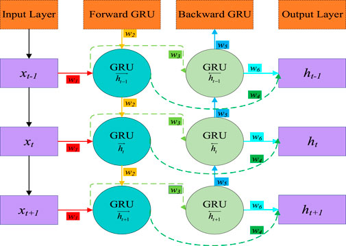
Figure 6. The Diagram of the BiGRU structure.

3.3 Attention mechanism

The attention mechanism is based on the workings of the human brain, where various parts are responsible for processing different types of information. Figure 7 illustrates how the attentional mechanism works. The formula for it is shown below from the Equations 28–30. This method enhances processing efficiency by focusing on significant elements, much like how our brain prioritizes information [28].

$e_i=u\tan h\left(\omega h_i+b\right)(28)$

${\alpha }_t=soft\max \left(e_t\right)=\frac{\mathit{exp}\left(e_t\right)}{{\displaystyle {\sum }_{j=1}^m}\mathit{exp}\left(e_j\right)}(29)$

$C={\displaystyle \sum _{j=1}^m}{\alpha }_j{h}_j(30)$

Figure 7

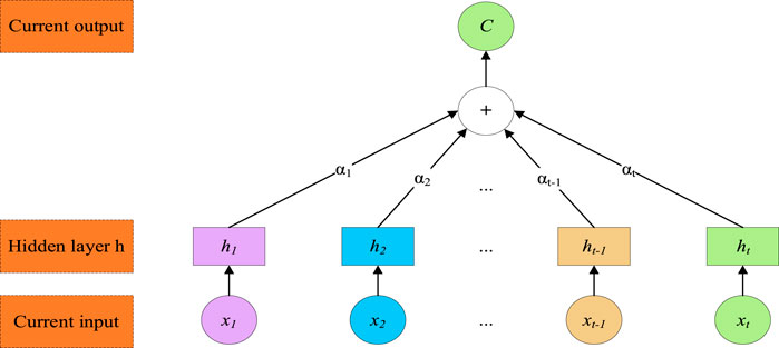
Figure 7. The structure of the attention unit.

3.4 SBOA-MIC-CBAM Hybrid Neural Network model

3.4.1 Maximal information coefficient

Maximal Information Coefficient (MIC) serves as a tool for quantifying the association existing between two characteristic variables. Its main idea is to divide the scatter plot of two related variables into grids. The probability density of the scatter points can be used to measure the mutual information coefficient between the two variables, thus capturing both linear and nonlinear associations. It belongs to an unsupervised learning method. Different ways of drawing grids will cause the samples to fall into different two-dimensional grids. By counting the number of scatter points in each grid interval and comparing it with the total number of samples, the joint distribution $p\left(x,y\right)$ of the grades and contents can be obtained. Combining with the characteristic marginal distribution $p\left(x\right)$ and the target marginal distribution $p\left(y\right)$, the relative entropy between the grade of the base wine and the substance content, that is, the mutual information $I\left(x,y\right)$, can be calculated via Equation 31 [8, 52]:

$MIC\left(x,y\right)=\underset{xy<B\left(n\right)}{\max }\frac{I\left(x,y\right)}{{\log }_2\left(\min \left(x,y\right)\right)}(31)$

$x,y$ represents two random variables; $xy<B$ and $B$ are the upper limits of the number of grids (functions of the sample size $n$, usually taking the value of $B=n^{0.6}$); $I\left(x,y\right)$ is the value of mutual information [8] expressed as the Equation 32:

$I\left(x,y\right)=\int p\left(x,y\right){\log }_2\frac{p\left(x,y\right)}{p\left(x\right)p\left(y\right)}\mathrm{d}x\mathrm{d}y(32)$

Through the normalization processing of MIC, it can be concluded that: the threshold value of MIC lies within the interval of [0, 1]. And when the threshold value of MIC is in the range of [0, 0.4), there is no correlation; when the threshold value of MIC is in the range of [0.4, 0.7), there is a correlation; when the threshold value of MIC is in the range of [0.7, 1), there is a strong correlation.

3.4.2 SBOA-CBAM neural network model

Figure 8 depicts how the CBA model is used to predict how many tourists will visit a scenic spot at a given time.

Figure 8

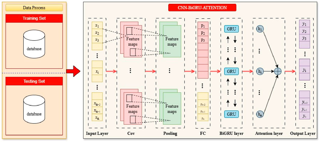
Figure 8. The structure of CNN-BiGRU-Attention model.

The SBOA-CBAM, designed for predicting tourist flow intervals in scenic spots, has five prediction steps; the detailed workflow is shown in Figure 9 [43].

Step 1: Data Preprocessing; Perform processing such as feature encoding and decomposition. The data that is screened by the MIC algorithm for importance is classified into two part, comprising 80% and 20% of the sample, respectively, one is used for training, and the other is used for testing. These sets are then normalized using the mapminmax method. This preprocessing step is crucial for effectively training and testing machine learning models. Normalization ensures that all data falls within a consistent range, preventing biases in the model’s performance.

Step 2: Hyperparameters model Optimization; The SBOA algorithm was employed to tune the parameter configurations for the CBA model in terms of the Initial Learning Rate, GRU Hidden Units, Global Dropout Probability, Attention Heads, Attention Output Dimension, Convolutional Filters, Convolutional Kernel Size, Fully-Connected Neurons, L2 Regularization Coefficient. After optimizing its hyperparameters with SBOA, the model was trained and evaluated using RMSE. If the RMSE was small, the optimal hyperparameters would be found; otherwise, the optimal hyperparameters would not be obtained, and the optimization process was repeated until the RMSE would reach a better value.

Step 3: Building of the optimized network; The optimized CBA network was built using the optimized hyperparameters from Step 2. Training parameters were set, the network was trained, and location prediction was performed.

Figure 9

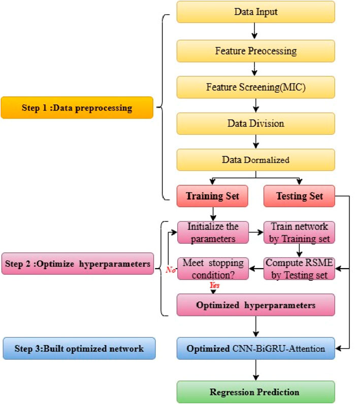
Figure 9. The workflow of SBOA-CBAM.

3.5 Evaluation criteria

This study employed five distinct methods to assess the accuracy of a tourist flow prediction model, aiming to forecast the number of visitors a scenic spot will receive. The methods used to measure accuracy include R², MSE, RMSE, MAE, MAPE. The formula for determining error can be found in sources [53, 54] and expressed by Equations 33–37:

$R^2=1-{\displaystyle \sum _{i=1}^N}{\left(y_i-{\widehat{y}}_i\right)}^2/{\displaystyle \sum _{i=1}^N}{\left(y_i-\overline{y}\right)}^2(33)$

$MSE=\frac{1}{N}{\displaystyle \sum _{i=1}^N}{\left(y_i-{\widehat{y}}_i\right)}^2(34)$

$RMSE=\sqrt{\frac{1}{N}{\displaystyle \sum _{i=1}^N}{\left(y_i-{\widehat{y}}_i\right)}^2}(35)$

$MAE=\frac{1}{N}{\displaystyle \sum _{i=1}^N}\left|y_i-{\widehat{y}}_i\right|\in [0,+\infty )(36)$

$MAPE=\frac{100\%}{N}{\displaystyle \sum _{i=1}^N}\left|\frac{y_i-{\widehat{y}}_i}{y_i}\right|(37)$

where, $y_i$ represents the real data, ${\widehat{y}}_i$ stands for the model’s estimates, N signifies the sample size, and $\overline{y}$ is the mean of the observed data.

4 Case analysis

4.1 Selection of fusion factors

Referring to references [4, 55], China’s Jiuzhaigou Valley was chosen as an illustration to prove the practicality of the suggested algorithm. The daily tourist flow data set of Jiuzhaigou Valley in China from 2012 to 2017 was chosen as the prediction data for the model. At the same time, factors such as the date $X_1$, season $X_2$, climatic characteristics $X_3$, temperature (maximum temperature $X_4$, minimum temperature $X_5$, average temperature $X_6$), holidays $X_7$, the tourist flow during the corresponding period of the previous year $X_8$, and seven network keywords (Jiuzhaigou Valley $X_9$, Jiuzhaigou Valley map $X_{10}$, scenic spots in Jiuzhaigou Valley $X_{11}$, hotels in Jiuzhaigou Valley $X_{12}$, travel guides for Jiuzhaigou Valley $X_{13}$, tickets for Jiuzhaigou Valley $X_{14}$, weather in Jiuzhaigou Valley $X_{15}$) are selected as the features for predicting the tourist flow in the scenic area.

4.1.1 Season

In order to verify whether the natural seasons of the environment affect the accuracy of tourist flow prediction, the 12 months of every year are partitioned into four segments in accordance with the four seasons: spring, summer, autumn, and winter. The following “multiple dummy variables” are introduced to represent different seasons [4], with S representing the seasons, and its encoding results can be expressed as Equation 38.

$\mathrm{S}=\left\{\begin{array}{l}\begin{array}{cc}1& \text{Spring}\end{array}\\ \begin{array}{cc}2& \text{Summer}\end{array}\\ \begin{array}{cc}3& \text{Autumn}\end{array}\\ \begin{array}{cc}4& \text{Winter}\end{array}\end{array}\right.(38)$

4.1.2 Climatic characteristics

In order to determine whether the weather and climate affect the accuracy of tourist flow prediction, three categories are used to classify the weather conditions: sunny, rainy days (heavy rain, torrential rain, sleet, light snow), and snowy days (heavy snow). The following “multiple dummy variables” are introduced to represent different weather conditions, with W representing the weather, and its encoding results can be expressed as Equation 39.

$W=\left\{\begin{array}{l}\begin{array}{cc}1& other\text{weather}\end{array}\\ \begin{array}{cc}4& \text{Rainy weather}\end{array}\\ \begin{array}{cc}7& \text{Snowy weather}\end{array}\end{array}\right.(39)$

4.1.3 Statutory holidays

Studies have shown that working days, weekends, statutory holidays, etc., have a certain impact on the daily tourist flow of scenic areas. In order to make the quantitative results better explain the influence of different holidays, this paper distinguishes the 365 days of the whole year according to working days, weekends, Labor Day, Spring Festival, National Day, and other statutory holidays, and introduces the following “multiple dummy variables” to represent different holidays, with H representing the holidays, and its encoding results can be expressed as Equation 40:

$H=\left\{\begin{array}{cc}0& Workday\\ 1& Weekend\\ 3& OthersLegalHoliday\\ 6& LabourDay\\ 9& SpringFestival,NationalDay\end{array}\right.(40)$

Special note: When weekends and statutory holidays form a continuous vacation, this paper defines it as a statutory holiday, and it will be processed according to the above model.

4.1.4 Baidu index

By synthesizing the keywords selected in literature such as [56], the keywords selected in this paper are determined as follows: Jiuzhaigou Valley (Index1), Jiuzhaigou Valley Map (Index2), Scenic Spots in Jiuzhaigou Valley (Index3), Hotels in Jiuzhaigou Valley (Index4), Travel Guides for Jiuzhaigou Valley (Index5), Tickets for Jiuzhaigou Valley (Index6), and Weather in Jiuzhaigou Valley (Index7). The daily network search data of these seven Baidu Indexes from 2013 to 2017 were extracted, as shown in the Figure 10.

Figure 10

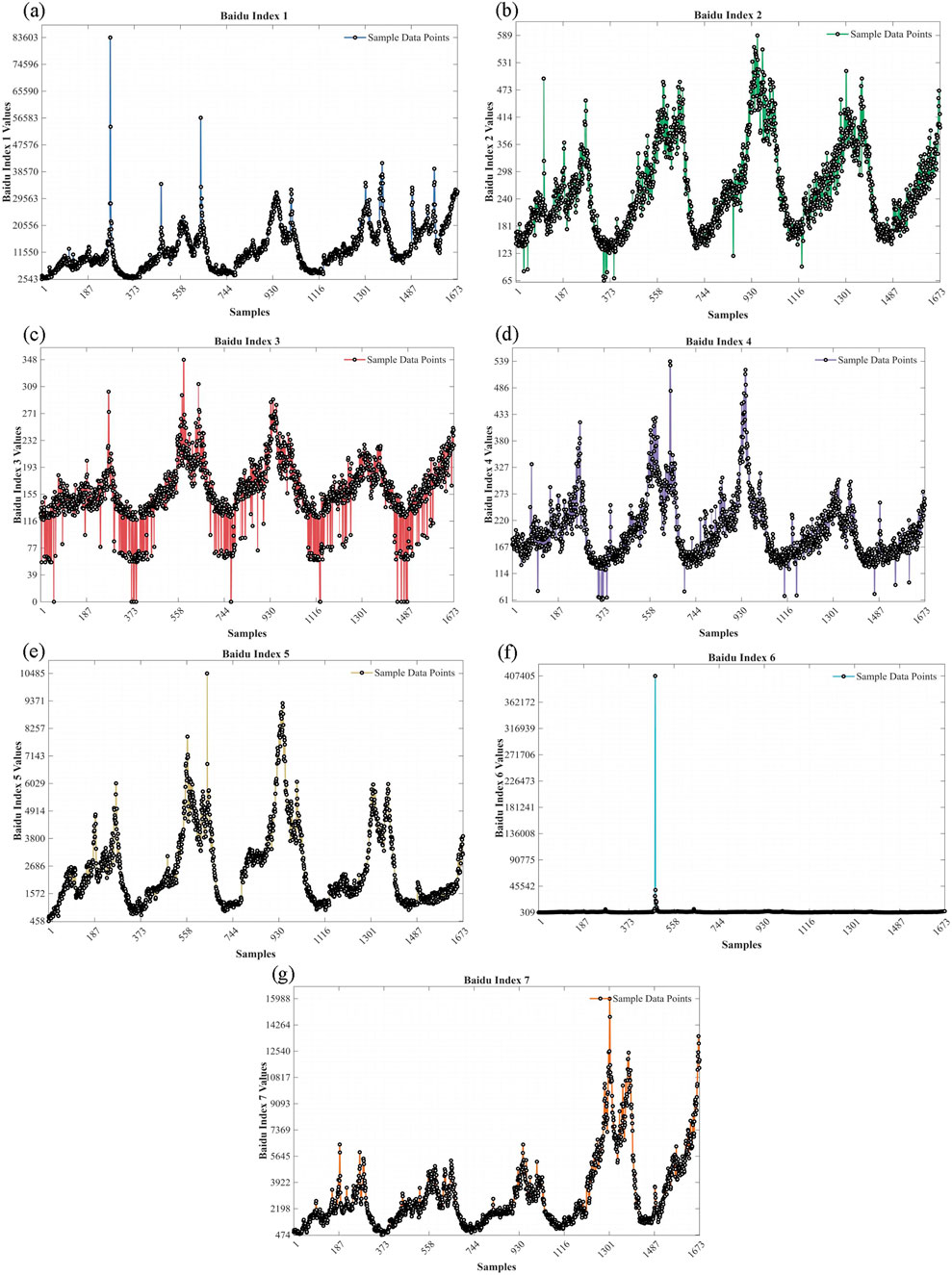
Figure 10. Network search data. (a) Jiuzhaigou Valley (Index1) (b) Jiuzhaigou Valley Map (Index2) (c) Scenic Spots in Jiuzhaigou Valley (Index3) (d) Hotels in Jiuzhaigou Valley (Index4) (e) Travel Guides for Jiuzhaigou Valley (Index5) (f) Tickets for Jiuzhaigou Valley (Index6) (g) Weather in Jiuzhaigou Valley (Index7).

4.2 Feature screening

This study focuses on analyzing the visitor flow at the Jiuzhaigou Valley Scenic and Historic Interest Area in China. In light of the tragic 7.0-magnitude earthquake that struck Jiuzhaigou County in 2017, causing the area to temporarily close for restoration and reconstruction, the Jiuzhaigou Scenic Area officially reopened on 12 July 2024. Therefore, this paper used the passenger flow of the Jiuzhaigou Scenic Area from 1 January 2013, to 8 August 2017, as the basic data to make the original data more convincing. The passenger flow of the Jiuzhaigou Scenic Area from 1 January 2013, to 31 July 2017, is shown in Figure 11.

Figure 11

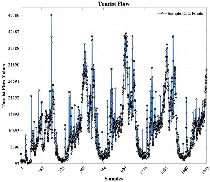
Figure 11. Passenger flow of Jiuzhaigou Valley Scenic and Historic Interest Area from 1 January 2013, to 31 July 2017, 2017.

4.2.1 Data Preprocessing

Date continuity validation supplements missing dates. Continuous variables adopt 7-day moving median imputation for missing values, categorical variables implement nearest-neighbor imputation for missing values, and the IQR method processes anomalies.

4.2.2 Feature engineering

• Temporal features: Date variables are decomposed into three fundamental variables: year, month, and day. Day-of-Year (DOY) and weekday ordinal are introduced as temporal features, with trigonometric encoding (sine/cosine transformation) applied to both.

• Meteorological features: A 5-day moving average temperature feature is introduced. Trapezoidal membership functions based on the pentadic temperature method calculate seasonal probability distributions by fuzzy logic.

• Holiday features: Statutory holidays are one-hot encoded while a dynamic window lag matrix (pre-/post-holiday markers) is constructed.

• Baidu indices: Baidu index features undergo adaptive period detection (ACF peak identification), STL decomposition (trend/seasonal/residual), and residual smoothing, significantly enhancing their information density.

• Tourist flow: Skewness detection is performed on previous-year’s tourist flow (Prev Year) and daily tourist flow (Tourist Flow). Features meeting threshold criteria undergo log10 (1+x) transformation, thus effectively improving distribution morphology.

4.2.3 Preliminary feature screening

The Maximal Information Coefficient (MIC) calculates nonlinear correlations between features and target variables across different lag steps. Initially screened features meeting criteria have their optimal lag orders extracted. The MIC coefficients and importance degrees of each feature are shown in Figure 12. According to literature [8] combined with the situation of the MIC coefficients in the Figure 12, the features with correlation coefficients greater than 0.3 are retained, and other features are eliminated, 14 features are retained. Table 1 represents the MIC coefficients of each feature, the lead times and the ranking results.

Figure 12

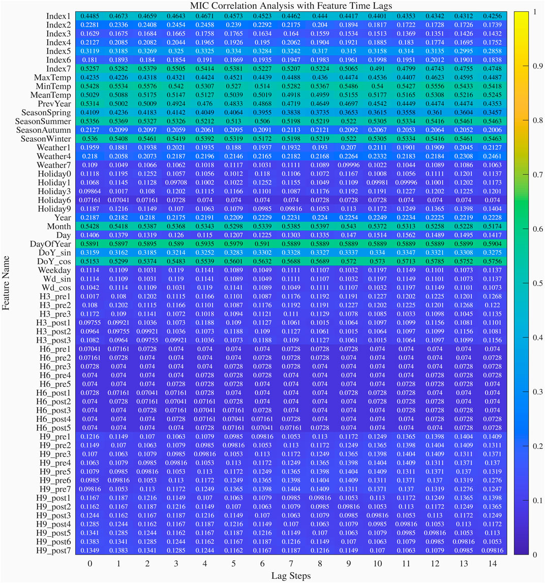
Figure 12. The MIC coefficients and importance degrees of each feature.

Table 1

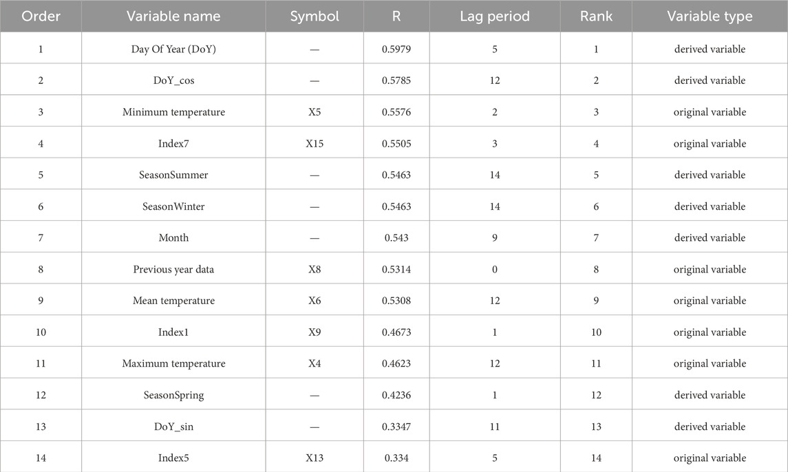
Table 1. MIC coefficients of selected feature, the lead times.

4.2.4 Feature refined screening

Based on preliminary MIC screening results, the feature matrix is reconstructed through PACF significance test. Expanding window cross-validation is employed to evaluate feature predictive capability for refined screening. This process retains only lag information from Baidu indices while forcibly preserving all derived variables of holiday features, thus ultimately reconstructing the final dataset.

At this stage, every input variable of the prediction model has been settled, and the function of the prediction model can be formulated as Equation 41.

$Y=F\left(X_4,X_5,X_6,X_8,X_9,X_{13},X_{15},\dots \right)(41)$

4.3 Data processing

The final dataset is classified into two parts, comprising 80% and 20% of the sample, one is used for training, and the other is used to testing, respectively. To ensure accurate analysis, a normalization technique was implemented to standardize the data within the range of [0,1]. The normalization equation used for this purpose can be succinctly expressed as Equation 42:

$x^{*}=\frac{x-x_{\min }}{x_{\max }-x_{\min }}(42)$

where $x*$ symbolizes the standardized data, $x$ stands for the original data, and $x_{\max }$ as well as $x_{\min }$ denote the maxima and minim, respectively, within the given example data.

4.4 Prediction model and results

To enhance the accuracy and reliability of the proposed tourism demand prediction model, this paper conducted a comparative analysis involving multiple models, including the CBA model, its SBOA-optimized variant (SBOA-CBA), BP neural network, SVM, and ELM. Basic parameters of each model are detailed in Table 2.

Table 2

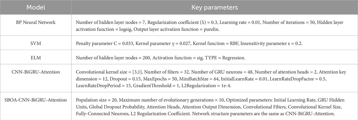
Table 2. Basic parameters of each mode.

The parameters of the CBA model were compared before and after optimization, with the results displayed in Table 3. This study highlights the significance of parameter optimization in improving the overall performance of predictive models.

Table 3

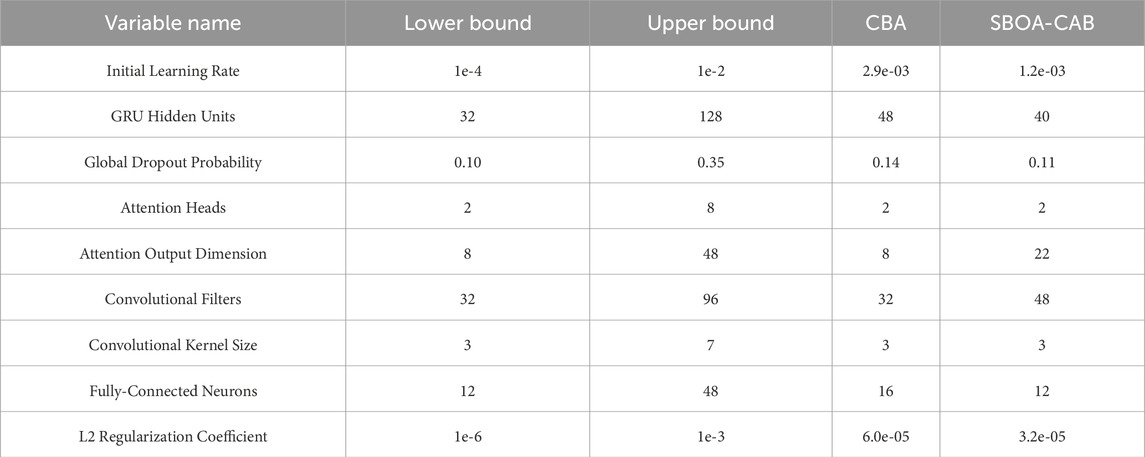
Table 3. CBA model parameters before and after optimization.

The prediction results and errors of the five models, namely, the CBA model, SBOA-CBA, BP neural network, SVM, and ELM, can be observed from Figures 13–16. Specifically, Figure 13 displays the prediction results of the five models on the training dataset, while Figure 14 illustrates the prediction errors of the five models for the training dataset. Figure 15 presents the prediction results of the five models on the testing dataset, and finally Figure 16 shows the prediction errors of the five models for the testing dataset. From the visualizations in Figures 13–16, the performance ranking of the models can be clearly ordered as follows: SBOA - CBA > CBA model > SVM > BP neural network > ELM. These visuals provide valuable insights into the performance comparison among the models.

Figure 13

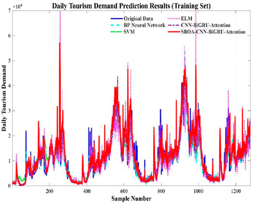
Figure 13. Predicted results (training set).

Figure 14

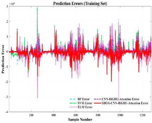
Figure 14. Predicted error (training set).

Figure 15

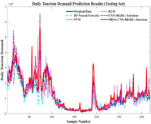
Figure 15. Predicted results (testing set).

Figure 16

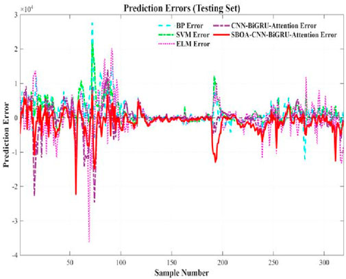
Figure 16. Predicted error (testing set).

The results of R², MAPE, MAE, MSE, and RMSE for the scenic spot tourist flow prediction models established using the Convolutional-Bidirectional-Attention Model (CBA), BP (Backpropagation Neural Network), SVM (Support Vector Machine), and ELM (Extreme Learning Machine) are presented in Table 4. Figures 17–19 show the visual comparisons of the R², MAPE, MAE, MSE and RMSE metrics among the five models.

Table 4

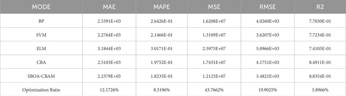
Table 4. CNN-BiGRU-ATTENTION evaluation indexes before and after optimization.

Figure 17

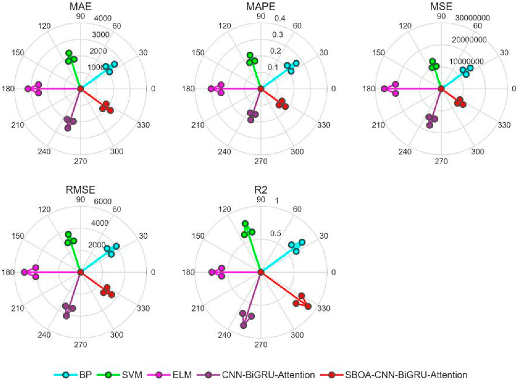
Figure 17. Radar chart of evaluation index.

Figure 18

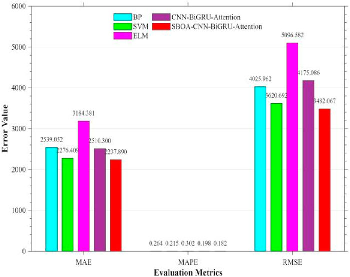
Figure 18. Histogram of evaluation indexes (MAE, MAPE, RMSE).

Figure 19

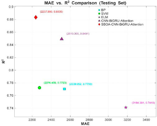
Figure 19. Scatter diagram of the evaluation indexes (R², MAE).

As can be seen from Figures 17–19 and Table 4, compared with the BP, SVM, and ELM models, the CBA model ranks first in both MAPE (19.75%) and R² (0.8491), indicating its significant advantages in terms of relative error control and overall goodness of fit. The improvement in R² shows that the CBA model can explain more than 84% of the variation in tourist flow, providing highly reliable inputs for subsequent resource scheduling and dynamic pricing. The significant reduction in MAPE (a 25.3% decrease compared with BP and a 34.5% decrease compared with ELM) directly meets the business demand for “percentage accuracy”. In terms of absolute error metrics, the MAE (2.5103 × 10³), MSE (1.7431 × 10⁷) and RMSE (4.1751 × 10³) of the CBA model are slightly lower than those of the SVM model but are 21.2%, 32.9% and 18.1% better than those of the ELM model, respectively. Meanwhile, the “suboptimal” performance of the absolute error metrics (MAE and RMSE) can be partially attributed to the natural occurrence of abnormal peaks in scenic spot tourist flow (such as extreme weather and emergencies). These outliers exert an asymmetric amplifying effect on both squared losses (MSE/RMSE) and absolute losses (MAE). Therefore, the leading performance of MAPE and R² is more valuable for decision-making than the absolute error metrics. Additionally, the CBA model extracts local spatiotemporal features of tourist flow sequences through convolutional layers, and then uses a bidirectional attention mechanism to capture long-range dependencies and external disturbances such as holidays. This not only maintains the interpretability of the model but also significantly reduces the risk of underfitting to high-dimensional nonlinearity, which is a common issue in traditional methods. Thus, there are sufficient theoretical and practical bases for adopting the CBA model as the benchmark model for scenic spot tourist flow prediction.

As can be seen from Figures 17–19 and Table 4, after globally optimizing 9 key hyperparameters of the CBA model, including Initial Learning Rate, GRU Hidden Units, Global Dropout Probability, Attention Heads, Attention Output Dimension, Convolutional Filters, Convolutional Kernel Size, Fully-Connected Neurons, and L2 Regularization Coefficient, using the Sandpiper-Bird Optimization Algorithm (SBOA), metrics such as R², MAPE, MAE, MSE, and RMSE have all been improved. The R² value increased from 0.8491 to 0.8835, with a growth rate of 3.90%, indicating a significant enhancement in the model’s ability to explain tourist flow fluctuations. The RMSE decreased from 4.1751 × 10³ to 3.4821 × 10³ (↓19.90%), the MSE dropped from 1.7431 × 10⁷ to 1.2125 × 10⁷ (↓43.77%), the MAE reduced from 2.5103 × 10³ to 2.2379 × 10³ (↓12.17%), and the MAPE declined from 0.1975 to 0.1824 (↓8.32%). By adaptively adjusting the learning rate and L2 regularization coefficient, the overfitting phenomenon was effectively suppressed. Through optimizing the convolutional kernel size and the number of filters, the convolutional layers maintained efficient computational performance while capturing multi-scale spatiotemporal features. By regulating the Attention Heads and Output Dimension, the model’s sensitivity to external shocks such as holidays and sudden weather changes was significantly enhanced. To summarize, the CBA model had already demonstrated better predictive performance than traditional algorithms in the initial comparison, while the SBOA-CBAM not only further reduced the prediction error but also significantly improved the model’s accuracy in characterizing the spatiotemporal nonlinear coupling of scenic spot tourist flow, providing scenic spot management departments with a more robust and real-time decision support tool.

4.5 Model stability testing

Section 2.5 conducted a comparative analysis evaluating the performance of SBOA, HOA, HHO, WOA, PSO and GA algorithms on a subset of the CEC2017 benchmark test functions. The results demonstrate that SBOA achieved the top rank among the tested functions, exhibiting superior optimization capability and high stability. This provides theoretical justification and relevant arguments for using SBOA to optimize the hyperparameters of the CNN-BiGRU-Attention model. To thoroughly validate the optimization effect and confirm that the SBOA-optimized model delivers stable and significant performance improvements compared to the original model, this study designed an experimental scheme of “single optimization followed by multiple training”, more precisely: After fixing the hyperparameters obtained via a single SBOA optimization run, 30 independent training sessions were conducted to compare the performance of the model before and after optimization. The specific implementation steps are as follows:

• Single Optimization: The SBOA algorithm was executed only once to obtain a fixed set of hyperparameters.

• Fixed Architecture and Data Partitioning: The architecture of the CNN-BiGRU-Attention model remained unchanged, and a fixed 80/20 training set/test set split was employed.

• Paired Initialization: Each training session utilized paired random seeds for weight initialization, ensuring experimental reproducibility and fair comparison.

• Statistical Evaluation: Using the test set’s Root Mean Square Error (RMSE) and Mean Absolute Error (MAE) as paired samples, a one-tailed Wilcoxon signed-rank test (significance level α = 0.05, testing the direction that the optimized model is superior) was performed. Cohen’s d effect size and its 95% Bootstrap confidence interval were calculated to quantify the strength of the optimization effect.

This scheme aims to comprehensively evaluate the optimized model’s performance stability, its disturbance resistance and its compatibility with the target architecture. The experimental results are presented in Table 5 and Figure 20.

Table 5

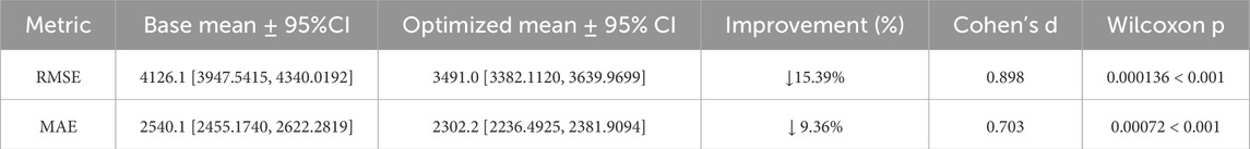
Table 5. Model Evaluation Results: Comparison Before vs. After Optimization (N = 30 Runs).

Figure 20

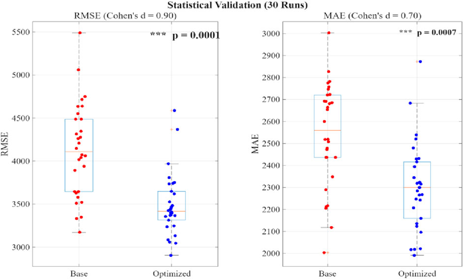
Figure 20. Boxplot of the evaluation indexes (MAE, RMSE).

Figure 20 presents the error distributions of the CBA and SBOA-CBA models across the 30 independent repeated experiments. The boxplots demonstrate that, compared to the pre-optimization model (red), the distributions of both RMSE and MAE for the optimized model (blue) exhibit a median reduction of approximately 15.39% and 9.36%, respectively. Furthermore, the overall downward shift of the box indicates a systematic reduction in the error.

The results from the 30 independent repeated experiments demonstrate a significant overall reduction in error on the test set for the SBOA-optimized CNN-BiGRU-Attention model. RMSE’s Mean decreased from 4,126.1 (95% CI: 3,947.5415–4,340.0192) to 3,491 (95% CI: 3,382.1120–3,639.9699), representing a 15.3930% reduction. Mae’s Mean decreased from 2,540.1 (95% CI: 2,455.1740–2,622.2819) to 2,302.2 (95% CI: 2,236.4925–2,381.9094), representing a 9.3626% reduction. The Wilcoxon signed-rank test indicated that the improvements in both metrics were highly statistically significant (RMSE: p = 0.0001; MAE: p = 0.0007). Effect size analysis further confirmed the practical significance of the optimization: Cohen’s d for RMSE = 0.8982 (large effect), Cohen’s d for MAE = 0.7028 (medium-to-large effect). In conclusion, the SBOA algorithm not only significantly improved the model’s prediction accuracy but also enhanced its stability and disturbance resistance.

5 Conclusion and future work

5.1 Major contribution

The sharp increase in tourists has resulted in congestion, overcrowding, safety-related incidents, and low tourist satisfaction. Real-time tracking and forecasting of tourist flow data in scenic spots can help managers plan resources more rationally, optimize services, and increase tourist satisfaction. At the same time, it can serve as a valuable resource for tourism planning. To address this problem, the SBOA-CBAM tourist flow prediction model was proposed. CNN captures the spatial feature relationship of past passenger flow information; BiGRU detects dynamic changes and pays attention to key features in conjunction with the attention mechanism, while the hyperparameters of the model were refined through the utilization of the SBAO algorithm. Ultimately, comparative simulation trials proved the efficiency of the SBAO - CBA algorithm. Here are the primary findings presented in this article:

1. Compared with BP, SVM, and ELM,the CBA model has been put forward with the aim of predicting tourist flows. The simulation demonstrated that the constructed model effectively captured the characteristics of tourist flow data that is screened by the MIC algorithm, making it suitable for this purpose.

2. The SBOA algorithm optimized the CBA parameters to improve prediction accuracy. The CBA model’s evaluation indexes include R², RMSE, MSE, MAE, and MAPE. The model improved every parameter: R² increased by 3.8966%, RMSE decreased by 19.9025%, MAE decreased by 12.1726%, MAPE decreased by 8.3196%, and MSE decreased by 43.7662%.

3. The Wilcoxon signed-rank test indicated that the improvements in both metrics were highly statistically significant (RMSE: p = 0.0001; MAE: p = 0.0007). Effect size analysis further confirmed the practical significance of the optimization: Cohen’s d for RMSE = 0.8982 (large effect), Cohen’s d for MAE = 0.7028 (medium-to-large effect). The SBOA algorithm not only significantly improved the model’s prediction accuracy but also enhanced its stability and disturbance resistance.

5.2 Limitations

Despite the promising results, this study has several limitations that warrant consideration:

1. Only the daily tourist flow data from Jiuzhaigou Scenic Area in Sichuan Province between 2013 and 2017 were selected as the foundational dataset for model training and testing. No updated data was introduced for validation analysis.

2. Only the daily tourist flow data from Jiuzhaigou Scenic Area in Sichuan Province were used as the training set and test set, without employing data from other regions to validate the model’s generalizability.

5.3 Future research direction

Although this study has achieved preliminary results in the task of predicting daily tourism demand, there are still some limitations, which can be improved and expanded in the future from the following directions:

1. Expanding the research scope to enhance the model’s generalizability. By incorporating data from more regions, it will be conducted an in-depth analysis of the model’s adaptability. Building upon this foundation, will further improve the model’s applicability to data from different regions through various approaches, such as adjusting the model architecture and optimizing model parameters. Specifically, the number of layers in the model, adjust the number of neurons in each layer, or alter the types of activation functions could be increased to more accurately fit the data characteristics of different regions. Furthermore, the model’s training efficiency and accuracy can be enhanced by tuning parameters such as the learning rate and optimization algorithms. Through these comprehensive measures, the goal is for the model to demonstrate stronger generalization capabilities and higher accuracy when confronted with data from diverse regions.

2. Integrating more features to improve model accuracy. It is essential to incorporate data from various tourist destinations, ensuring these destinations encompass a broad spectrum of geographical, cultural and economic backgrounds. By integrating this diverse data, the validity and relevance of the data samples can be improved, thereby improving the model’s precision. This approach will facilitate a more comprehensive understanding and analysis of tourism market trends, tourist demands and behavioral patterns, thus providing more robust support and guidance for the development of the tourism industry.

6 Policy implications

The SBOA-CBAM prediction model, integrating network search index data, can provide accurate forecasts of tourism demand. This capability not only serves as a valuable reference for tourist travel planning but also assists managers in rationally allocating resources, reducing energy consumption and waste generation, and implementing crowd control measures. Consequently, it helps alleviate ecological stress on scenic areas, safeguarding the long-term sustainable development of local tourism. Furthermore, the model provides a critical reference basis for scientific decision-making by tourism management departments, thereby advancing sustainable tourism development strategies. Specifically, it yields the following three policy implications:

1. Tourist scenic areas can draw on the passenger flow prediction method in this paper to establish a passenger flow early warning model and an early warning platform, and promptly release passenger flow prediction information to business operators and tourists. This can effectively guide tourists to travel during off-peak periods and guide operators to make proper reception and response arrangements.

2. Government management departments can utilize the model prediction to grasp the future passenger flow situation in the region, effectively adjust the supply of the tourism market and supervise the carrying capacity of the tourism ecological environment.

3. Tourism development departments can also analyze the changing trends of the tourism market further by using the passenger flow data predicted by the model and make full preparations for the next-step tourism planning and resource mobilization.

Data availability statement

The original contributions presented in the study are included in the article/supplementary material, further inquiries can be directed to the corresponding author.

Author contributions

ZW: Conceptualization, Data curation, Funding acquisition, Methodology, Writing – original draft, Writing – review and editing. PH: Conceptualization, Methodology, Writing – review and editing. SY: Data curation, Software, Writing – original draft.

Funding

The author(s) declare that financial support was received for the research and/or publication of this article. This research was Supported by Sichuan Science and Technology Program (No. 2023JDR0239).

Conflict of interest

The authors declare that the research was conducted in the absence of any commercial or financial relationships that could be construed as a potential conflict of interest.

Generative AI statement

The author(s) declare that no Generative AI was used in the creation of this manuscript.

Any alternative text (alt text) provided alongside figures in this article has been generated by Frontiers with the support of artificial intelligence and reasonable efforts have been made to ensure accuracy, including review by the authors wherever possible. If you identify any issues, please contact us.

Publisher’s note

All claims expressed in this article are solely those of the authors and do not necessarily represent those of their affiliated organizations, or those of the publisher, the editors and the reviewers. Any product that may be evaluated in this article, or claim that may be made by its manufacturer, is not guaranteed or endorsed by the publisher.

References

1. Ni T, Wang L, Zhang P, Wang B, Li W. Daily tourist flow forecasting using SPCA and CNN-LSTM neural network. Concurrency Comput Pract Exper (2021) 33:e5980. doi:10.1002/cpe.5980

CrossRef Full Text | Google Scholar

2. Dai L, Wang H. An improved WOA (whale optimization algorithm)-based CNN-BIGRU-CBAM model and its application to short-term power load forecasting. Energies (2024) 17:2559. doi:10.3390/en17112559

CrossRef Full Text | Google Scholar

3. Chen J, Ying Z, Zhang C, Balezentis T. Forecasting tourism demand with search engine data: a hybrid CNN-BiLSTM model based on boruta feature selection. Inf Process Manage (2024) 61:103699. doi:10.1016/j.ipm.2024.103699

CrossRef Full Text | Google Scholar

4. Li K, Liang C, Lu W, Li C, Zhao S, Wang B. Forecasting of short-term daily tourist flow based on seasonal clustering method and PSO-LSSVM. ISPRS Int J Geo-inf (2020) 9:676. doi:10.3390/ijgi9110676

CrossRef Full Text | Google Scholar

5. Qin X, Yin D, Dong X, Chen D, Zhang S. Passenger flow prediction of scenic spots in jilin province based on convolutional neural network and improved quantile regression long short-term memory network. ISPRS Int J Geo-inf (2022) 11:509. doi:10.3390/ijgi11100509

CrossRef Full Text | Google Scholar

6. Meng Q, Dou Y. Research on short-term forecast of railway passenger volume based on EMD-CNN-LSTM model. Railw Transp Econ (2023) 45:64–73. doi:10.16668/j.cnki.issn.1003-1421.2023.12.09

CrossRef Full Text | Google Scholar

7. Constantino HA, Fernandes PO, Teixeira JP. Tourism demand modelling and forecasting with artificial neural network models: the Mozambique case study. Tékhne (2016) 14:113–24. doi:10.1016/j.tekhne.2016.04.006

CrossRef Full Text | Google Scholar

8. Wang H, Liu W. Forecasting tourism demand by a novel multi-factors fusion approach. IEEE Access (2022) 10:125972–91. doi:10.1109/ACCESS.2022.3225958

CrossRef Full Text | Google Scholar

9. Lu W, Rui H, Liang C, Jiang L, Zhao S, Li K. A method based on GA-CNN-LSTM for daily tourist flow prediction at scenic spots. Entropy (2020) 22:261. doi:10.3390/e22030261

PubMed Abstract | CrossRef Full Text | Google Scholar

10. Gao Z, Zhang J, Xu Z, Zhang X, Shi R, Wang J, et al. Method of predicting passenger flow in scenic areas considering multisource traffic data. Sens Mater (2020) 32:3907. doi:10.18494/SAM.2020.2970

CrossRef Full Text | Google Scholar

11. Gu F, Jiang K, Ding Y. Predicting urban tourism flow with tourism digital footprints based on deep learning. KSII TIIS (2023) 17:1162–81. doi:10.3837/tiis.2023.04.007

CrossRef Full Text | Google Scholar

12. Liu S, Lin W, Wang Y, Yu DZ, Peng Y, Ma X. Convolutional neural network-based bidirectional gated recurrent unit–additive attention mechanism hybrid deep neural networks for short-term traffic flow prediction. Sustainability (2024) 16:1986. doi:10.3390/su16051986

CrossRef Full Text | Google Scholar

13. Cho K, Merrienboer B, Gülçehre Ç, Bahdanau D, Bougares F, Schwenk H, et al. Learning phrase representations using RNN encoder–decoder for statistical machine translation. In: Conference on empirical methods in natural language processing (2014). p. 1724–34. doi:10.3115/v1/D14-1179

CrossRef Full Text | Google Scholar

14. Yang C, Ran Q, Luo D, Dou W. CNN-BIGRU short-term electricity price prediction based on attention mechanism. Proc Csu-epsa (2024) 36:22–9. doi:10.19635/j.cnki.csu-epsa.001257

CrossRef Full Text | Google Scholar

15. Hussain B, Afzal MK, Ahmad S, Mostafa AM. Intelligent traffic flow prediction using optimized GRU model. IEEE Access (2021) 9:100736–46. doi:10.1109/ACCESS.2021.3097141

CrossRef Full Text | Google Scholar

16. Jeong M-H, Lee T-Y, Jeon S-B, Youm M. Highway speed prediction using gated recurrent unit neural networks. Appl Sci (2021) 11:3059. doi:10.3390/app11073059

CrossRef Full Text | Google Scholar

17. Ren C, Chai C, Yin C, Ji H, Cheng X, Gao G, et al. Short-term traffic flow prediction: a method of combined deep learnings. J Adv Transp (2021) 2021:1–15. doi:10.1155/2021/9928073

CrossRef Full Text | Google Scholar

18. Yang Y-Q, Lin J, Zheng Y-B. Short-time traffic forecasting in tourist service areas based on a CNN and GRU neural network. Appl Sci (2022) 12:9114. doi:10.3390/app12189114

CrossRef Full Text | Google Scholar

19. Yuan L, Zeng Y, Chen H, Jin J. Terminal traffic situation prediction model under the influence of weather based on deep learning approaches. Aerospace (2022) 9:580. doi:10.3390/aerospace9100580

CrossRef Full Text | Google Scholar

20. Chai C, Ren C, Yin C, Xu H, Meng Q, Teng J, et al. A multifeature fusion short-term traffic flow prediction model based on deep learnings. J Adv Transp (2022) 2022:1–13. doi:10.1155/2022/1702766

CrossRef Full Text | Google Scholar

21. Chen Y, Xiao J-W, Wang Y-W, Luo Y. Non-crossing quantile probabilistic forecasting of cluster wind power considering spatio-temporal correlation. Appl Energy (2025) 377:124356. doi:10.1016/j.apenergy.2024.124356

CrossRef Full Text | Google Scholar

22. Shuang R, Yang K, Shang J, Qi J, Xiangyu W, Cai Y. Short-term power load forecasting based on CNN-BiGRU-attention. J Electr Eng (2024) 19:344–50. doi:10.11985/2024.01.037

CrossRef Full Text | Google Scholar

23. Na F, Jun-jie Y, Jun-xiao L, Chang W. Short-term power load forecasting based on CNN-BIGRU-ATTENTION. Comput Simul (2022) 39:40–4. doi:10.3969/j.issn.1006-9348.2022.02.008

CrossRef Full Text | Google Scholar

24. Niu D, Yu M, Sun L, Gao T, Wang K. Short-term multi-energy load forecasting for integrated energy systems based on CNN-BiGRU optimized by attention mechanism. Appl Energy (2022) 313:118801. doi:10.1016/j.apenergy.2022.118801

CrossRef Full Text | Google Scholar

25. Xingang C, Long Z, Zhipeng M, Song L, Zhixian Z. State of health assessment of lithium batteries based on ISSA-CNN-BiGRU-attention. Electron Meas Technol (2024) 47:45–52. doi:10.19651/j.cnki.emt.2415653

CrossRef Full Text | Google Scholar

26. Sun W, Chen J, Hu C, Lin Y, Wang M, Zhao H, et al. Clock bias prediction of navigation satellite based on BWO-CNN-BiGRU-attention model. GPS Solutions (2025) 29:46. doi:10.1007/s10291-024-01809-1

CrossRef Full Text | Google Scholar

27. Wu K, Chen H, Li L, Liu Z, Chang H. Position prediction for space teleoperation with SAO-CNN-BiGRU-attention algorithm. IEEE Robot Autom Lett (2024) 9:11674–81. doi:10.1109/LRA.2024.3498700

CrossRef Full Text | Google Scholar

28. Yuan Q, Yu P, Tan L, Wang Y, Zhang H. Research on short-term power load forecasting model based on NGO-CNN-BIGRU-AT. IAENG Int J Comput Sci (2024) 51:1163–70.

Google Scholar

29. Duan Y, Li C, Wang X, Guo Y, Wang H. Forecasting influenza trends using decomposition technique and LightGBM optimized by grey wolf optimizer algorithm. Mathematics (2024) 13:24. doi:10.3390/math13010024

CrossRef Full Text | Google Scholar

30. Zhou W, Huang D, Liang Q, Huang T, Wang X, Pei H, et al. Early warning and predicting of COVID-19 using zero-inflated negative binomial regression model and negative binomial regression model. BMC Infect Dis (2024) 24:1006. doi:10.1186/s12879-024-09940-7

PubMed Abstract | CrossRef Full Text | Google Scholar

31. Guo Y, Zhang L, Pang S, Cui X, Zhao X, Feng Y. Deep learning models for hepatitis E incidence prediction leveraging baidu index. BMC Public Health (2024) 24:3014. doi:10.1186/s12889-024-20532-7

PubMed Abstract | CrossRef Full Text | Google Scholar

32. Dong W, Chen R, Ba X, Zhu S. Trend forecasting of public concern about low carbon based on comprehensive baidu index and its relationship with CO2 emissions: the case of China. Sustainability (2023) 15:12973. doi:10.3390/su151712973

CrossRef Full Text | Google Scholar

33. Pan B, Chenguang Wu D, Song H. Forecasting hotel room demand using search engine data. J Hosp Tour Technol (2012) 3:196–210. doi:10.1108/17579881211264486

CrossRef Full Text | Google Scholar

34. Li X, Pan B, Law R, Huang X. Forecasting tourism demand with composite search index. Tour Manag (2017) 59:57–66. doi:10.1016/j.tourman.2016.07.005

CrossRef Full Text | Google Scholar

35. Pan B, MacLaurin T, Crotts JC. Travel blogs and the implications for destination marketing. J Trav Res. (2007) 46:35–45. doi:10.1177/0047287507302378

CrossRef Full Text | Google Scholar

36. Fu Y, Liu D, Chen J, He L. Secretary bird optimization algorithm: a new metaheuristic for solving global optimization problems. Artif Intell Rev (2024) 57:123. doi:10.1007/s10462-024-10729-y

CrossRef Full Text | Google Scholar

37. Qin S, Liu J, Bai X, Hu G. A multi-strategy improvement secretary bird optimization algorithm for engineering optimization problems. Biomimetics (2024) 9:478. doi:10.3390/biomimetics9080478

PubMed Abstract | CrossRef Full Text | Google Scholar

38. Oladejo SO, Ekwe SO, Mirjalili S. The hiking optimization algorithm: a novel human-based metaheuristic approach. Knowledge-based Syst (2024) 296:111880. doi:10.1016/j.knosys.2024.111880

CrossRef Full Text | Google Scholar

39. Heidari AA, Mirjalili S, Faris H, Aljarah I, Mafarja M, Chen H. Harris hawks optimization: algorithm and applications. Future Gener Comput Syst (2019) 97:849–72. doi:10.1016/j.future.2019.02.028

CrossRef Full Text | Google Scholar

40. Mirjalili S, Lewis A. The whale optimization algorithm. Adv Eng Softw (2016) 95:51–67. doi:10.1016/j.advengsoft.2016.01.008

CrossRef Full Text | Google Scholar

41. Kennedy J, Eberhart R. Particle swarm optimization. In: Proceedings of ICNN’95 - international conference on neural networks. Perth, WA, Australia: IEEE (1995). p. 1942–8. doi:10.1109/ICNN.1995.488968

CrossRef Full Text | Google Scholar

42. Holland J. Genetic algorithms. Scientific Am (1992) 267:66–72. doi:10.1038/scientificamerican0792-66

CrossRef Full Text | Google Scholar

43. Yu Y, Han X, Yang M, Yang J. Probabilistic prediction of regional wind power based on spatiotemporal quantile regression. IEEE Trans Ind Appl (2020) 56:6117–27. doi:10.1109/TIA.2020.2992945

CrossRef Full Text | Google Scholar

44. Chiu M-C, Hsu H-W, Chen K-S, Wen C-Y. A hybrid CNN-GRU based probabilistic model for load forecasting from individual household to commercial building. Energy Rep (2023) 9:94–105. doi:10.1016/j.egyr.2023.05.090

CrossRef Full Text | Google Scholar

45. Gu B, Li X, Xu F, Yang X, Wang F, Wang P. Forecasting and uncertainty analysis of day-ahead photovoltaic power based on WT-CNN-BiLSTM-AM-GMM. Sustainability (2023) 15:6538. doi:10.3390/su15086538

CrossRef Full Text | Google Scholar

46. Liu H, Ma T, Lin Y, Peng K, Hu X, Xie S, et al. Deep learning in rockburst intensity level prediction: performance evaluation and comparison of the NGO-CNN-BiGRU-attention model. Appl Sci (2024) 14:5719. doi:10.3390/app14135719

CrossRef Full Text | Google Scholar

47. Zhu M, Yu X, Tan H, Yuan J, Chen K, Xie S, et al. High-precision monitoring and prediction of mining area surface subsidence using SBAS-InSAR and CNN-BiGRU-attention model. Sci Rep (2024) 14:28968. doi:10.1038/s41598-024-80446-7

PubMed Abstract | CrossRef Full Text | Google Scholar

48. Meng Y, Chang C, Huo J, Zhang Y, Mohammed Al-Neshmi HM, Xu J, et al. Research on ultra-short-term prediction model of wind power based on attention mechanism and CNN-BiGRU combined. Front Energy Res (2022) 10:920835. doi:10.3389/fenrg.2022.920835

CrossRef Full Text | Google Scholar

49. Bi X, Zhang T. Pedagogical sentiment analysis based on the BERT-CNN-BiGRU-attention model in the context of intercultural communication barriers. Peerj Comput Sci (2024) 10:e2166. doi:10.7717/peerj-cs.2166

PubMed Abstract | CrossRef Full Text | Google Scholar

50. Li X, Ding L, Du Y, Fan Y, Shen F. Position-enhanced multi-head self-attention based bidirectional gated recurrent unit for aspect-level sentiment classification. Front Psychol (2022) 12:799926–2021. doi:10.3389/fpsyg.2021.799926

PubMed Abstract | CrossRef Full Text | Google Scholar

51. Zhu D, Wei Y, Cai J, Wang J, Chen Z. A security data detection and management method in digital library network based on deep learning. Front Phys (2024) 12:1492114. doi:10.3389/fphy.2024.1492114

CrossRef Full Text | Google Scholar

52. Cova D, Liu Y. Shear wave velocity prediction using bidirectional recurrent gated graph convolutional network with total information embeddings. Front Earth Sci (2023) 11:1101601–2023. doi:10.3389/feart.2023.1101601

CrossRef Full Text | Google Scholar

53. Fu S, Zhu R, Yu F. Research on predictive analysis method of building energy consumption based on TCN-BiGru-attention. Appl Sci (2024) 14:9373. doi:10.3390/app14209373

CrossRef Full Text | Google Scholar

54. Guo W, Xu L, Wang T, Zhao D, Tang X. Photovoltaic power prediction based on hybrid deep learning networks and meteorological data. Sens. (2024) 24:1593. doi:10.3390/s24051593

PubMed Abstract | CrossRef Full Text | Google Scholar

55. Wang W, Chen J, Zhang Y, Gong Z, Kumar N, Wei W. A multi-graph convolutional network framework for tourist flow prediction. ACM Trans Internet Technol (2021) 21:1–13. doi:10.1145/3424220

CrossRef Full Text | Google Scholar

56. Wu B, Wang L, Tao R, Zeng Y-R. Interpretable tourism volume forecasting with multivariate time series under the impact of COVID-19. Neural Comput Appl (2023) 35:5437–63. doi:10.1007/s00521-022-07967-y

PubMed Abstract | CrossRef Full Text | Google Scholar