A nonlocal advection system for two competing species with resources recovering time

Competitive interactions between multiple cell populations are crucial for modeling biological processes such as tumor growth and tissue regeneration. In this study, we investigate the nonlocal advection model for two-species competition, which characterizes cell growth and dispersion phenomena in co-culture experiments. To capture realistic phenomena in biology, we introduce the time delay representing population migration and resources recovering time. The primary objectives are to investigate the impact of time delays on competitive dynamics under various parameter settings and to develop numerical methods that ensure biological feasibility of solutions. Accordingly, we design a positivity-preserving finite volume scheme based on an upwind flux approach, guaranteeing non-negative population densities and discrete conservation properties. We examine the convergence orders of the scheme through the numerical experiments and explore the effects of time delays on species competition dynamics under different parameter settings.

1 Introduction

The mathematical modeling of multi-species population dynamics provides a theoretical framework for studying species interactions in biological and ecological systems [1, 2]. In biochemical research, scientists employ co-culture systems to elucidate competitive relationships between distinct cell types, such as cancer cells and normal cells [3]. Early models included nonlinear diffusion and reaction-diffusion systems [4, 5, 6], revealing that spatial segregation can promote species coexistence by mitigating interspecific competition. A key approach in modern models involves nonlocal advection systems [7, 8], where population movement is influenced by long-range interactions instead of purely local diffusion. These models are often associated with chemotaxis, the directed movement of cells or organisms along chemical concentration gradients [9, 10, 11, 12]. The well-posedness of nonlocal advection models for two species (or a single species) has been studied in [7, 8, 13, 14]. Moreover, nonlocal advection systems are closely connected to continuum models of pedestrian dynamics, where an individual’s velocity is influenced not only by local density but also by spatially distributed crowd information [15, 16]. Extensions considering anisotropic interactions and domain boundaries further demonstrate the relevance of nonlocal frameworks to realistic crowd flow modeling [17, 18].

Time delays capture the inherent non-instantaneous nature of biological processes, yielding more realistic models that can exhibit oscillatory, bifurcation, and stability behaviors observed in real systems [19, 20]. Following the pioneering work of [21], numerous studies have introduced time delays in population dynamics models. In single species models such as the delayed logistic model [22, 23, 24], the delay represents the maturation time before individuals become reproductively active and can destabilize population dynamics by inducing oscillations or periodic behavior once it exceeds a critical threshold. The time delayed Lotka–Volterra predator-prey model [25, 23, 26] incorporates the predator’s delayed response to changes in prey population, enabling more accurate simulations of periodic oscillations and stability shifts in ecosystems. Time lags in competition models [27, 28] physically represent ecological processes such as resource recovery or interspecific interaction lags, and they can destabilize equilibrium states to induce stable periodic oscillations or even chaotic dynamics through Hopf bifurcation or period-doubling bifurcations.

This study aims to extend the existing nonlocal advection model for two competing species by incorporating time delays. Previous studies focused on population mobility and interactions, while our study introduces time delays to characterize the interaction between population migration and resource recovery. To ensure biologically realistic population densities, we develop a positivity-preserving finite volume scheme. We conduct extensive numerical experiments to: (1) examine the numerical convergence orders; (2) investigate the influence of time delays on competitive dynamics under various parameter settings.

In this work, we first introduce the mathematical model—the two species hyperbolic Keller–Segel system with time delays, and then design a finite volume scheme satisfying the positivity-preserving property, where we adopt the upwind type flux similar to [29–32, 33]. We investigate the experimental convergence orders of the proposed scheme. According to the numerical simulation, under various parameter settings, we find that small, identical delays in both species lead to a steady state, whereas larger delays may induce unsteady and potentially the extinction of one or both species. Moreover, asymmetric delay parameters between the two species tend to confer a competitive advantage to one species.

The rest of this paper is organized as follows. In Section 2, we extend the nonlocal advection Keller–Segel model by incorporating time delay and develop a positivity-preserving finite volume method that also satisfies discrete conservation laws. Numerical examples are presented in Section 3.

2 The mathematical model and the finite volume scheme

In this section, we introduce the time delay to the classical hyperbolic Keller–Segel system and design a positivity-preserving finite volume scheme.

2.1 PDE model

We consider the nonlocal advection system for two competing species with time delays in an interval $I=[a,b]$. We denote by $u_j(t,x)(j=\mathrm{1,2})$ the density of two species. The PDE model is stated as follows.

${\partial }_t{u}_1-d_1{\partial }_x\left(u_1{\partial }_{x}p\right)=u_1{h}_{1,{\alpha }_1}\left(u_1,u_2\right)\text{in\hspace{0.17em}}\left(0,T\right]\times I,(\mathrm{2.1a})$

${\partial }_t{u}_2-d_2{\partial }_x\left(u_2{\partial }_{x}p\right)=u_2{h}_{2,{\alpha }_2}\left(u_1,u_2\right)\text{in\hspace{0.17em}}\left(0,T\right]\times I,(\mathrm{2.1b})$

$\left(I-\chi \mathrm{\Delta }\right)p=u_1+u_2\text{in\hspace{0.17em}}\left(0,T\right]\times I,(\mathrm{2.1c})$

${\partial }_{x}p\left(t,a\right)={\partial }_{x}p\left(t,b\right)=0\text{on\hspace{0.17em}}\left(0,T\right],(\mathrm{2.1d})$

$u_1\left(t,x\right)=u_{\mathrm{1,0}}\left(x\right)\text{\hspace{0.17em}in\hspace{0.17em}}I,t\le 0,(2.1e)$

$u_2\left(t,x\right)=u_{\mathrm{2,0}}\left(x\right)\text{\hspace{0.17em}in\hspace{0.17em}}I,t\le 0,(\mathrm{2.1f})$

where $\nu$ is the outward normal vector, $d_j(j=\mathrm{1,2})$ is the dispersion coefficient, $\chi$ is the sensing coefficient. The function $p(t,x)$, which represents the pressure or chemical potential field induced by species densities, satisfies the elliptic Equations 2.1c, 2.1d, and its gradient ${\partial }_{x}p$ influences the movement direction of the species $u_j(j=\mathrm{1,2})$. We set, for ${\alpha }_1,{\alpha }_2\ge 0$,

$h_{1,{\alpha }_1}\left(\left(u_1,u_2\right)\left(t,x\right)\right)=b_1-{\delta }_1-\left(a_{11}{u}_1\left(t-{\alpha }_1,x\right)+a_{12}{u}_2\left(t,x\right)\right),(\mathrm{2.2a})$

$h_{2,{\alpha }_2}\left(\left(u_1,u_2\right)\left(t,x\right)\right)=b_2-{\delta }_2-\left(a_{21}{u}_1\left(t,x\right)+a_{22}{u}_2\left(t-{\alpha }_2,x\right)\right),(\mathrm{2.2b})$

where $b_j>0(j=\mathrm{1,2})$ are the growth rates, $a_{jj}\ge 0(j=\mathrm{1,2})$ represent the intraspecific competition coefficients, reflecting competition between individuals of the same species, $a_{12},a_{21}\ge 0$ denote the interspecific competition coefficients between species, ${\alpha }_j\ge 0(j=\mathrm{1,2})$ represent the delay parameters, and ${\delta }_j(j=\mathrm{1,2})$ are the additional mortality rates caused by drug treatment. The delay parameters ${\alpha }_j$ in $h_{j,{\alpha }_j}(j=\mathrm{1,2})$ represent time lags in intraspecific competition of species $u_j(j=\mathrm{1,2})$, reflecting delayed self-density feedback from migration and resource recovery. When ${\alpha }_1={\alpha }_2=0$, Equations 2.1a–2.1f is the hyperbolic Keller–Segel system proposed in [14].

2.2 The finite volume scheme

We introduce the fully discrete finite volume scheme for problem Equations 2.1a–2.1f. We hereafter denote by $|\omega |$ the measure of the interval $\omega$ in $\mathbb{R}$.

2.2.1 The finite volume scheme

For simplicity, we divide the computational domain $I=[a,b]$ into $N_c$ cells (see Figure 1):

$C_i=\left\{x:x_{i-\frac{1}{2}}\le x\le x_{i+\frac{1}{2}}\right\},1\le i\le N_c,$

where

$a=x_{\frac{1}{2}}<x_{\frac{3}{2}}<\cdots <x_{N_c+\frac{1}{2}}=b.$

We denote by $x_i=(x_{i+\frac{1}{2}}+x_{i-\frac{1}{2}})/2$ the center of the cell $C_i$, and set

$h_i=x_{i+\frac{1}{2}}-x_{i-\frac{1}{2}}\left(1\le i\le N_c\right),h=\underset{1\le i\le N_c}{\max }{h}_i.$

We introduce the space of the piecewise constant function:

${\mathcal{V}}_h=\left\{v_h\in L^{\infty }\left(I\right):v_h{|}_{C_i}\in P_0\left(C_i\right)\text{for\hspace{0.17em}\hspace{0.17em}all\hspace{0.17em}\hspace{0.17em}}{C}_i\right\},$

where $P_0(C_i)$ represents the set of constant functions in cell $C_i$.

Figure 1

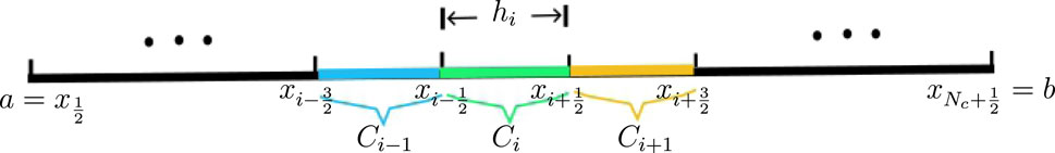
Figure 1. The mesh for the interval $I$.

We assume that there are two integers $M_1$ and $M_2$ such that the delay parameters satisfy ${\alpha }_2=(M_2/M_1){\alpha }_1$. Let $\tau ={\alpha }_1/(K{M}_1)$ for some integer K. We can take the integers $m_1=K{M}_1$, $m_2=K{M}_2$. Then we see that ${\alpha }_1=m_1\tau$, ${\alpha }_2=m_2\tau$.

Let $N$ be the smallest integer such that $N\tau \ge T$. The time interval is divided into $N$ segments:

$0=t_0<t_1<\cdots <t_n<t_{n+1}<\cdots <t_N,\text{\hspace{0.17em}with\hspace{0.17em}}{t}_n=n\tau ,$

and we use the backward Euler to approximate time-differential, i.e.,

${\partial }_{\tau }{v}^n≔\frac{v^n-v^{n-1}}{\tau }\approx v_t\left(t_n\right)\left(v^n=v\left(t_n\right)\right).$

Let $p_h^n,u_{1,h}^n,u_{2,h}^n\in {\mathcal{V}}_h$ be the numerical approximation to $p(t_n,x),u_1(t_n,x),u_2(t_n,x)$ $(n=\mathrm{0,1},\dots ,N)$. The proposed scheme is described below.

By integrating Equations 2.1a–2.1c on each cell $C_i$ and applying integration by parts, we obtain the following implicit scheme at $t=t_n$ using the backward Euler method:

$\begin{array}{cc}\hfill & {\left.{\int }_{C_i}p\left(t_n,x\right)dx-\left(\chi {\partial }_{x}p\left(t_n,x\right)\right)\right|}_{x_{i-\frac{1}{2}}}^{x_{i+\frac{1}{2}}}={\int }_{C_i}\left(u_1\left(t_{n-1},x\right)+u_2\left(t_{n-1},x\right)\right)dx,\hfill \\ \hfill & {\left.{\int }_{C_i}{\partial }_t{u}_1\left(t_n,x\right)dx-\left(d_1{u}_1\left(t_n,x\right){\partial }_{x}p\left(t_n,x\right)\right)\right|}_{x_{i-\frac{1}{2}}}^{x_{i+\frac{1}{2}}}={\int }_{C_i}{u}_1\left(t_n,x\right)h_{1,{\alpha }_1}\left(\left(u_1,u_2\right)\left(t_{n-1},x\right)\right)dx,\hfill \\ \hfill & {\left.{\int }_{C_i}{\partial }_t{u}_2\left(t_n,x\right)dx-\left(d_2{u}_2\left(t_n,x\right){\partial }_{x}p\left(t_n,x\right)\right)\right|}_{x_{i-\frac{1}{2}}}^{x_{i+\frac{1}{2}}}={\int }_{C_i}{u}_2\left(t_n,x\right)h_{2,{\alpha }_2}\left(\left(u_1,u_2\right)\left(t_{n-1},x\right)\right)dx.\hfill \end{array}$

Using $p^n(x)\approx p_h^n(x_i)≔p_i^n,u_1^n(x)\approx u_{1,h}^n(x_i)≔u_{1,i}^n,u_2^n(x)\approx u_{2,h}^n(x_i)≔u_{2,i}^n$ on $C_i$, we get:

$\begin{array}{cc}\hfill & {\left.{\int }_{C_i}p\left(t_n,x\right)dx\approx |C_i|p_i^n,{\partial }_{x}p\left(t_n,x\right)\right|}_{x_{i-\frac{1}{2}}}^{x_{i+\frac{1}{2}}}={\partial }_{x}p\left(t_n,x_{i+\frac{1}{2}}\right)-{\partial }_{x}p\left(t_n,x_{i-\frac{1}{2}}\right),\hfill \\ \hfill & {\int }_{C_i}\left(u_1\left(t_{n-1},x\right)+u_2\left(t_{n-1},x\right)\right)dx\approx |C_i|\left(u_{1,i}^{n-1}+u_{2,i}^{n-1}\right),\hfill \\ \hfill & {\int }_{C_i}{\partial }_t{u}_j\left(t_n\right)dx\approx {\int }_{C_i}{\partial }_t{u}_{j,h}^n\left(x_i\right)dx=|C_i|{\partial }_t{u}_{j,i}^n=|C_i|\frac{u_{j,i}^n-u_{j,i}^{n-1}}{\tau }(j=\mathrm{1,2}),\hfill \\ \hfill & {\int }_{C_i}{u}_j\left(t_n,x\right)h_{j,{\alpha }_j}\left(\left(u_1,u_2\right)\left(t_{n-1},x\right)\right)dx\approx |C_i|u_{j,i}^n{h}_{j,{\alpha }_j}\left(u_{1,i}^{n-1},u_{2,i}^{n-1}\right)(j=\mathrm{1,2}).\hfill \end{array}$

We use the approximation:

${\mathbf{P}}_{i-\frac{1}{2}}^n≔{\partial }_{x}p\left(t_n,x_{i-\frac{1}{2}}\right)\approx \left\{\begin{array}{cccc}\hfill & \frac{p_i^n-p_{i-1}^n}{|x_i-x_{i-1}|}\hfill & \hfill & 2\le i\le N_c,\hfill \\ \hfill & 0\hfill & \hfill & i\in \left\{1,N_c+1\right\}\hfill \end{array}\right.(2.3)$

(by Equation 2.1d)

We apply the upwind discretization to treat the flux: for $j=\mathrm{1,2}$,

$\begin{array}{cc}\hfill & {\left.-\left(d_j{u}_j\left(t_n,x\right){\partial }_{x}p\left(t_n,x\right)\right)\right|}_{x_{i-\frac{1}{2}}}^{x_{i+\frac{1}{2}}}\approx F_{j,i+\frac{1}{2}}^n-F_{j,i-\frac{1}{2}}^n,\hfill \\ \hfill & F_{j,i-\frac{1}{2}}^n≔u_{j,i-1}^n{\left[-d_j{\mathbf{P}}_{i-\frac{1}{2}}^n\right]}^{+}-u_{j,i}^n{\left[-d_j{\mathbf{P}}_{i-\frac{1}{2}}^n\right]}^{-},\hfill \end{array}$

where ${[r]}^{+}=\max \{r,0\}$ and ${[r]}^{-}=\max \{-r,0\}$. The upwind type numerical flux can be understood as follows. If the “flux” is from $C_{i-1}$ towards $C_i$ (i.e., $-d_j{\mathbf{P}}_{i-\frac{1}{2}}^n>0$), then the numerical flux for $F_{j,i-\frac{1}{2}}^n$ is chosen as $u_{j,i-1}^n(-d_j{\mathbf{P}}_{i-\frac{1}{2}}^n)$; otherwise, we take $u_{j,i}^n(-d_j{\mathbf{P}}_{i-\frac{1}{2}}^n)$.

For simplicity, we set the notations:

$G_i^{n-1}≔u_{1,i}^{n-1}+u_{2,i}^{n-1},E_{j,i}^n≔u_{j,i}^n{h}_{j,{\alpha }_j}\left(u_{1,i}^{n-1},u_{2,i}^{n-1}\right)(j=\mathrm{1,2}).$

The time delay terms $h_{j,{\alpha }_j}(u_{1,i}^{n-1},u_{2,i}^{n-1})(j=\mathrm{1,2})$ are approximated by

$\begin{array}{cc}\hfill & h_{1,{\alpha }_1}\left(u_{1,i}^{n-1},u_{2,i}^{n-1}\right)=b_1-{\delta }_1-\left(a_{11}{u}_{1,i}^{n-1-m_1}+a_{12}{u}_{2,i}^{n-1}\right),\hfill \\ \hfill & h_{2,{\alpha }_2}\left(u_{1,i}^{n-1},u_{2,i}^{n-1}\right)=b_2-{\delta }_2-\left(a_{21}{u}_{1,i}^{n-1}+a_{22}{u}_{2,i}^{n-1-m_2}\right),\hfill \end{array}$

where the integers $m_j(j=\mathrm{1,2})$ satisfy

$t_{n-1}-{\alpha }_j=\left(n-1-m_j\right)\tau .$

For $1\le i\le N_c$, by the fact that $|C_i|=h_i$, we get the finite volume scheme (FVM) scheme.

$p_i^n-\frac{\chi }{h_i}\left({\mathbf{P}}_{i+\frac{1}{2}}^n-{\mathbf{P}}_{i-\frac{1}{2}}^n\right)=G_i^{n-1},(\mathrm{2.4a})$

$u_{1,i}^n+\frac{\tau }{h_i}\left(F_{1,i+\frac{1}{2}}^n-F_{1,i-\frac{1}{2}}^n\right)+\tau E_{1,i}^n=u_{1,i}^{n-1},(\mathrm{2.4b})$

$u_{2,i}^n+\frac{\tau }{h_i}\left(F_{2,i+\frac{1}{2}}^n-F_{2,i-\frac{1}{2}}^n\right)+\tau E_{2,i}^n=u_{2,i}^{n-1}.(\mathrm{2.4c})$

2.2.2 Positivity-preserving property

In this section, we show the positivity-preserving for the discrete solutions. We set ${\mathit{u}}_{j,h}^n={(u_{j,1}^n,\dots ,u_{j,N_c}^n)}^{\top }$.

Theorem 2.1. Assume that ${\mathit{u}}_{j,h}^k$ ($k\le n-1$, $j=\mathrm{1,2}$) are nonnegative and not identically zero. If $\tau$ is sufficiently small such that $\tau <\min \{\frac{1}{b_1-{\delta }_1},\frac{1}{b_2-{\delta }_2}\}$, then we have:

${\mathit{u}}_{1,h}^n\ge 0,{\mathit{u}}_{2,h}^n\ge 0\left(\forall n\ge 1\right).$

Proof. The discrete system Equations 2.4b, 2.4c can be rewritten into the matrix forms:

${\mathcal{A}}_j^n{\mathit{u}}_{j,h}^n={\mathit{u}}_{j,h}^{n-1}(j=\mathrm{1,2}),$

where ${\mathcal{A}}_j^n={(a_{j;i,s})}_{1\le i,s\le N_c}$,

$\begin{array}{cc}\hfill & a_{j;i,s}=\left\{\begin{array}{cccc}\hfill & 1+\frac{\tau }{h_i}{\left[-d_j{\mathbf{P}}_{i+\frac{1}{2}}^n\right]}^{+}+\frac{\tau }{h_i}{\left[-d_j{\mathbf{P}}_{i-\frac{1}{2}}^n\right]}^{-}-\tau h_{j,{\alpha }_j}\left(u_{1,i}^{n-1},u_{2,i}^{n-1}\right)\hfill & \hfill & s=i,\hfill \\ \hfill & -\frac{\tau }{h_i}{\left[-d_j{\mathbf{P}}_{i+\frac{1}{2}}^n\right]}^{-}\hfill & \hfill & s=i+1,\hfill \\ \hfill & -\frac{\tau }{h_i}{\left[-d_j{\mathbf{P}}_{i-\frac{1}{2}}^n\right]}^{+}\hfill & \hfill & s=i-1,\hfill \\ \hfill & 0\hfill & \hfill & \text{otherwise}.\hfill \end{array}\right.\hfill \end{array}$

We assume that ${\mathit{u}}_{j,h}^k\ge 0,\ne 0$ ($k\le n-1$, $j=\mathrm{1,2}$). In view of Equations 2.2a, 2.2b, we see that $h_{j,{\alpha }_j}(u_{1,i}^{n-1},u_{2,i}^{n-1})\le b_j-{\delta }_j(j=\mathrm{1,2})$. If we choose $\tau <\min \{\frac{1}{b_1-{\delta }_1},\frac{1}{b_2-{\delta }_2}\}$, then we obtain:

$1-\tau h_{j,{\alpha }_j}\left(u_{1,i}^{n-1},u_{2,i}^{n-1}\right)\ge 1-\tau \left(b_j-{\delta }_j\right)>0\left(j=\mathrm{1,2}\right).$

The following statements hold for ${\mathcal{A}}_j^n$.

1. ${\mathcal{A}}_j^n$ has positive diagonal entries, i.e., for $j=\mathrm{1,2}$ and $1\le i\le N_c$,

$1+\frac{\tau }{h_i}{\left[-d_j{\mathbf{P}}_{i+\frac{1}{2}}^n\right]}^{+}+\frac{\tau }{h_i}{\left[-d_j{\mathbf{P}}_{i-\frac{1}{2}}^n\right]}^{-}-\tau h_{j,{\alpha }_j}\left(u_{1,i}^{n-1},u_{2,i}^{n-1}\right)>0.$

2. ${\mathcal{A}}_j^n$ has non-positive off-diagonal entries, i.e., for $j=\mathrm{1,2}$ and $1\le i\le N_c$,

$-\frac{\tau }{h_i}{\left[-d_j{\mathbf{P}}_{i+\frac{1}{2}}^n\right]}^{-}\le 0,-\frac{\tau }{h_i}{\left[-d_j{\mathbf{P}}_{i-\frac{1}{2}}^n\right]}^{+}\le 0.$

3. All the column sums of ${\mathcal{A}}_j^n$ are positive, i.e., for $j=\mathrm{1,2}$ and $1\le i\le N_c$,

$a_{j;i-1,i}+a_{j;i,i}+a_{j;i+1,i}=1-\tau h_{j,{\alpha }_j}\left(u_{1,i}^{n-1},u_{2,i}^{n-1}\right)\ge 1-\tau \left(b_j-{\delta }_j\right)>0.$

According to a convenient sufficient but not necessary condition of M-matrices (cf. [5, Appendix]), we conclude that ${\mathcal{A}}_j^n$ is an M-matrix.

According to the properties of M-matrices, this implies that ${({\mathcal{A}}_j^n)}^{-1}>0$ $(j=\mathrm{1,2})$. Noting that ${\mathit{u}}_{j,h}^k\ge 0,\ne 0$ ($k\le n-1$, $j=\mathrm{1,2}$), we have ${\mathit{u}}_{j,h}^n={({\mathcal{A}}_j^n)}^{-1}{\mathit{u}}_{j,h}^{n-1}\ge 0$. By induction, we conclude that ${\mathit{u}}_{j,h}^n\ge 0$ $(j=\mathrm{1,2})$ for all $n$.

2.2.3 The discrete conservation laws

The purpose of this section is to establish the mass conservation property of the (FVM) scheme (see Equations 2.4a–2.4c).

Theorem 2.2. Let $u_{j,h}^n(j=\mathrm{1,2})$ be the solution of (FVM). Then, we have the discrete conservation law:

${\displaystyle \sum _{i=1}^{N_c}}{u}_{j,i}^n-{\displaystyle \sum _{i=1}^{N_c}}{u}_{j,i}^{n-1}={\displaystyle \sum _{i=1}^{N_c}}\tau E_{j,i}^n\left(j=\mathrm{1,2}\right).$

Moreover, under the assumptions that $h_{j,{\alpha }_j}=0$ $(j=\mathrm{1,2})$, it follows that

${\displaystyle \sum _{i=1}^{N_c}}{u}_{j,i}^n={\displaystyle \sum _{i=1}^{N_c}}{u}_{j,i}^0\left(j=\mathrm{1,2}\right).$

Proof. Summing up Equations 2.4b, 2.4c with respect to $i$, we obtain

${\displaystyle \sum _{i=1}^{N_c}}{u}_{j,i}^n+{\displaystyle \sum _{i=1}^{N_c}}\frac{\tau }{h_i}\left(F_{j,i+\frac{1}{2}}^n-F_{j,i-\frac{1}{2}}^n\right)+{\displaystyle \sum _{i=1}^{N_c}}\tau E_{j,i}^n={\displaystyle \sum _{i=1}^{N_c}}{u}_{j,i}^{n-1}\left(j=\mathrm{1,2}\right).$

We see that

${\displaystyle \sum _{i=1}^{N_c}}\frac{\tau }{h_i}\left(F_{j,i+\frac{1}{2}}^n-F_{j,i-\frac{1}{2}}^n\right)=\frac{\tau }{h_i}\left(F_{j,N_c+\frac{1}{2}}^n-F_{j,\frac{1}{2}}^n\right)\left(j=\mathrm{1,2}\right),$

where

$\begin{array}{cc}\hfill & F_{j,\frac{1}{2}}^n=u_{j,0}^n{\left[-d_j{\mathbf{P}}_{\frac{1}{2}}^n\right]}^{+}-u_{j,1}^n{\left[-d_j{\mathbf{P}}_{\frac{1}{2}}^n\right]}^{-}=0\hfill \\ \hfill & F_{j,N_c+\frac{1}{2}}^n=u_{j,N_c}^n{\left[-d_j{\mathbf{P}}_{N_c+\frac{1}{2}}^n\right]}^{+}-u_{j,N_c+1}^n{\left[-d_j{\mathbf{P}}_{N_c+\frac{1}{2}}^n\right]}^{-}=0\hfill \end{array}$

(by Equation 2.3).

Hence, we have

${\displaystyle \sum _{i=1}^{N_c}}{u}_{j,i}^n-{\displaystyle \sum _{i=1}^{N_c}}{u}_{j,i}^{n-1}={\displaystyle \sum _{i=1}^{N_c}}\tau E_{j,i}^n\left(j=\mathrm{1,2}\right).$

Moreover, if we assume that $h_{j,{\alpha }_j}=0$ (i.e., $E_{j,i}^n=0$), then we have

${\displaystyle \sum _{i=1}^{N_c}}{u}_{j,i}^n={\displaystyle \sum _{i=1}^{N_c}}{u}_{j,i}^{n-1}={\displaystyle \sum _{i=1}^{N_c}}{u}_{j,i}^0\left(j=\mathrm{1,2}\right).$

Hence the proof is complete.

Remark 2.3. For hyperbolic systems, there exist other positivity-preserving strategies, such as the linear scaling limiter [35, 36], which enforces bounds in finite volume and discontinuous Galerkin methods through constraints at Legendre Gauss-Lobatto points.

3 Numerical experiments

In this section, we conduct extensive numerical experiments, where we examine the numerical convergence orders, compare the results with the classical hyperbolic Keller–Segel system, and investigate the influence of time delays on competitive dynamics under various parameter settings. We take ${\delta }_j=0(j=\mathrm{1,2})$ in this section. We set.

$\Vert v{\Vert }_{L^2\left(I\right),{\mathcal{V}}_h}={\left({\displaystyle \sum _{i=1}^{N_c}}|v\left(x_i\right){|}^2|C_i|\right)}^{\frac{1}{2}}\forall v\in {\mathcal{V}}_h,$

$|v{|}_{H^1\left(I\right),{\mathcal{V}}_h}={\left({\displaystyle \sum _{i=1}^{N_c}}\frac{|v\left(x_i\right)-v\left(x_{i-1}\right){|}^2}{|x_i-x_{i-1}|}\right)}^{\frac{1}{2}}\forall v\in {\mathcal{V}}_h,$

$\Vert v{\Vert }_{H^1\left(I\right),{\mathcal{V}}_h}={\left(\Vert v{\Vert }_{L^2\left(I\right),{\mathcal{V}}_h}^2+|v{|}_{H^1\left(I\right),{\mathcal{V}}_h}^2\right)}^{\frac{1}{2}}\forall v\in {\mathcal{V}}_h.$

3.1 Example 1 (non-segregated initial functions)

We set $I=[-\mathrm{2,2}]$, $\chi =1$, $d_1=4$, $d_2=1$, and

$\begin{array}{cc}\hfill & h_{1,{\alpha }_1}\left(\left(u_1,u_2\right)\left(t,x\right)\right)=1-u_1\left(t-{\alpha }_1,x\right)-2u_2\left(t,x\right),\hfill \\ \hfill & h_{2,{\alpha }_2}\left(\left(u_1,u_2\right)\left(t,x\right)\right)=1-2u_1\left(t,x\right)-u_2\left(t-{\alpha }_2,x\right).\hfill \end{array}$

The initial conditions are chosen as follows:

$\begin{array}{cc}\hfill & \begin{array}{c}\hfill u_1\left(t,x\right)=\left\{\begin{array}{cccc}\hfill & 0.25-x^2\hfill & \hfill & -0.5\le x\le 0.5\hfill \\ \hfill & 0\hfill & \hfill & \text{otherwise}\hfill \end{array}\right.\text{for\hspace{0.17em}all\hspace{0.17em}}t\le 0,\end{array}\hfill \\ \hfill & \begin{array}{c}\hfill u_2\left(t,x\right)=\left\{\begin{array}{cccc}\hfill & 2\left(0.25-x^2\right)\hfill & \hfill & -0.5\le x\le 0.5\hfill \\ \hfill & 0\hfill & \hfill & \text{otherwise}\hfill \end{array}\right.\text{for\hspace{0.17em}all\hspace{0.17em}}t\le 0.\end{array}\hfill \end{array}$

To examine the influence of time delays on competitive dynamics under varying parameter settings, the following cases are considered.

1. the classical hyperbolic Keller–Segel system

$•$ Example 1-1: ${\alpha }_1={\alpha }_2=0$;

2. ${\alpha }_1={\alpha }_2$

$•$ Example 1-2-1: ${\alpha }_1={\alpha }_2=0.1$;

$•$ Example 1-2-2: ${\alpha }_1={\alpha }_2=0.5$;

$•$ Example 1-2-3: ${\alpha }_1={\alpha }_2=1.5$;

$•$ Example 1-2-4: ${\alpha }_1={\alpha }_2=2$;

$•$ Example 1-2-5: ${\alpha }_1={\alpha }_2=5$;

3. ${\alpha }_1\ne {\alpha }_2$

$•$ Example 1-2-6: ${\alpha }_1=0.5,{\alpha }_2=1$;

$•$ Example 1-2-7: ${\alpha }_1=1,{\alpha }_2=0.5$;

$•$ Example 1-2-8: ${\alpha }_1=0.5,{\alpha }_2=1.5$;

$•$ Example 1-2-9: ${\alpha }_1=1.5,{\alpha }_2=0.5$.

To obtain the experimental convergence order of the mesh size $h$, we fix $\tau =\frac{1}{2000}$, use the numerical solution with $h=\frac{1}{2000}$ at $T=1$ as the reference solution (denoted by ($u_{1,ref}^N$, $u_{2,ref}^N$, $p_{\mathit{ref}}^N$)), and compute the errors for different mesh sizes $h=\frac{1}{80},\frac{1}{160},\frac{1}{320},\frac{1}{640}$. For the classical hyperbolic Keller–Segel system (i.e., ${\alpha }_1={\alpha }_2=0$), the experimental errors are shown in Table 1. For the system with time delay $({\alpha }_1={\alpha }_2=0.5)$, the experimental errors are presented in Table 2. We observe the first-order convergence with respect to the mesh size $h$ for $\Vert u_{j,ref}^N-u_{j,h}^N{\Vert }_{L^2(I),{\mathcal{V}}_h}$ $(j=\mathrm{1,2})$ and $\Vert p_{\mathit{ref}}^N-p_h^N{\Vert }_{H^1(I),{\mathcal{V}}_h}$.

Table 1

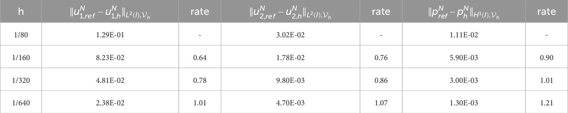
Table 1. Experimental errors and convergence order of $h$ for ${\alpha }_1={\alpha }_2=0$ (Example 1-1).

Table 2

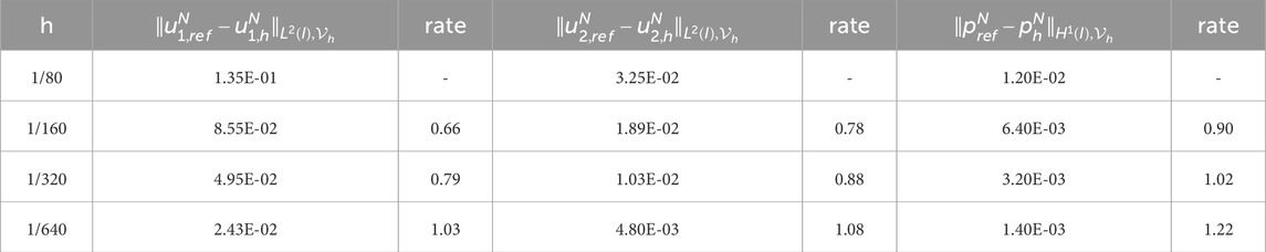
Table 2. Experimental errors and convergence order of $h$ for ${\alpha }_1={\alpha }_2=0.5$ (Example 1-2-2).

The evolution of the solutions for the classical hyperbolic Keller–Segel system (i.e., ${\alpha }_1={\alpha }_2=0$) with $h=\tau =\frac{1}{1000}$ is shown in Figure 2. The solution dynamics of the time-delayed nonlocal advection model with $h=\tau =\frac{1}{1000}$ are presented in Figures 3–6. We classify the dynamic behaviors for ${\alpha }_1={\alpha }_2$ and ${\alpha }_1\ne {\alpha }_2$ in Tables 3, 4, respectively. For the non-segregated initial function cases, small symmetric delays $({\alpha }_1={\alpha }_2\le 0.5)$ lead to steady coexistence (see Example 1-2-1 – Example 1-2-2, Figure 3), while larger delays $({\alpha }_1={\alpha }_2\ge 1.5)$ cause unsteady dynamics and potential extinction of one or both species (see Example 1-2-3 – Example 1-2-5, Figure 4). When the time delay is identical for both species (i.e., ${\alpha }_1={\alpha }_2$) and sufficiently large, the delayed competitive feedback leads to an unsteady system. The populations overreact to outdated density information, causing oscillations that eventually drive both species to extinction, as seen in the numerical results. For the case with asymmetric delays, we observe that the species with the larger delay is dominance in the competition (e.g., $u_2$ dominates when ${\alpha }_1<{\alpha }_2$, or vice versa (see Example 1-2-6 – Example 1-2-9, Figures 5, 6)).

Figure 2

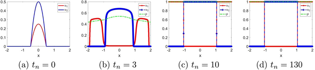
Figure 2. The numerical solution for ${\alpha }_1={\alpha }_2=0$ (Example 1-1). (a–d) show the evaluation of the numerical solution at different times.

Figure 3

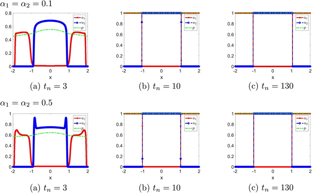
Figure 3. The numerical solution (Examples 1-2-1, 1-2-2). (a–c) show the evaluation of the numerical solution at different times.

Figure 4

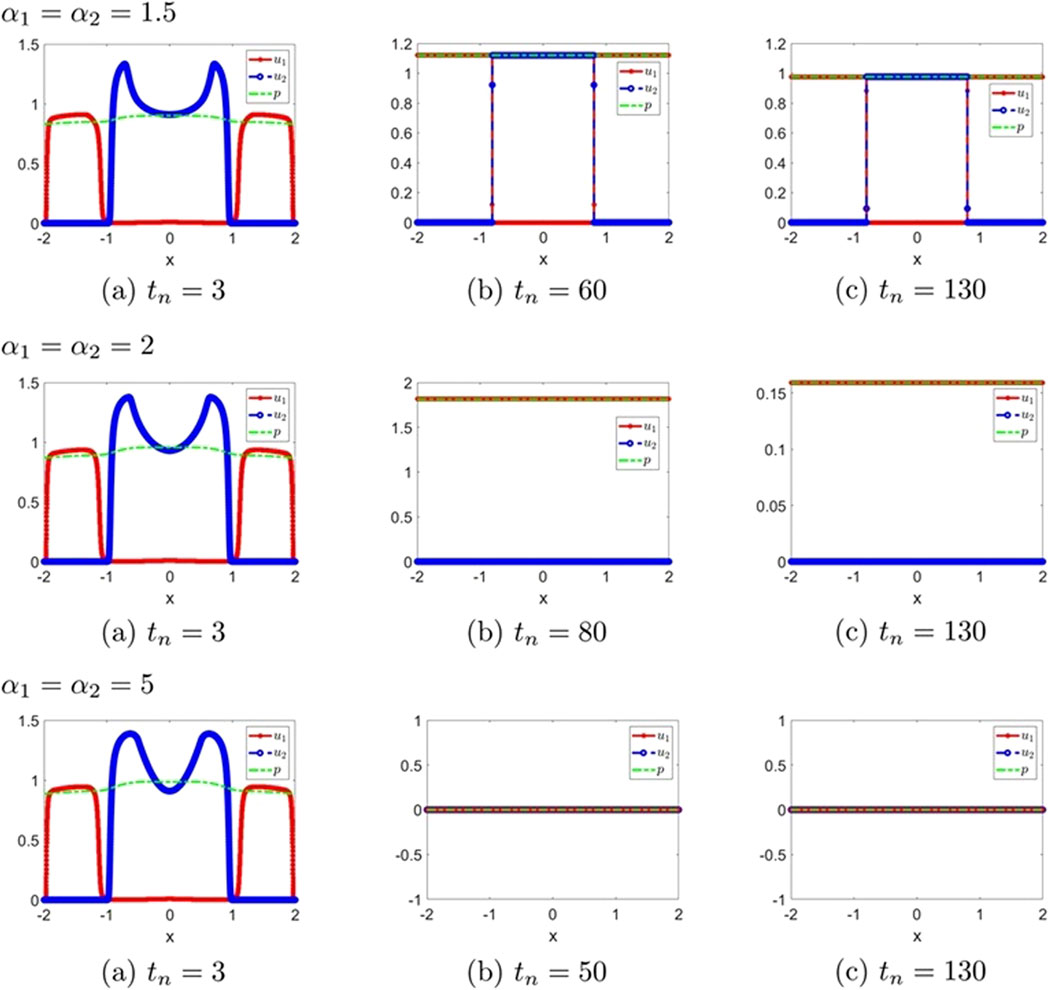
Figure 4. The numerical solution (Examples 1-2-3, 1-2-4, 1-2-5). (a–c) show the evaluation of the numerical solution at different times.

Figure 5

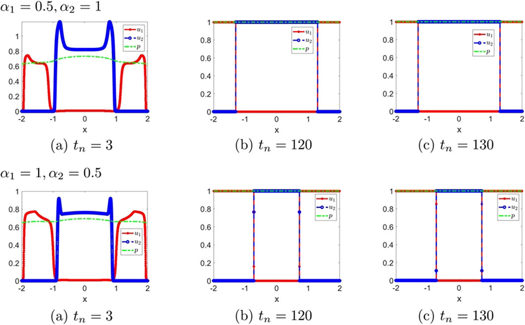
Figure 5. The numerical solution (Examples 1-2-6, 1-2-7). (a–c) show the evaluation of the numerical solution at different times.

Figure 6

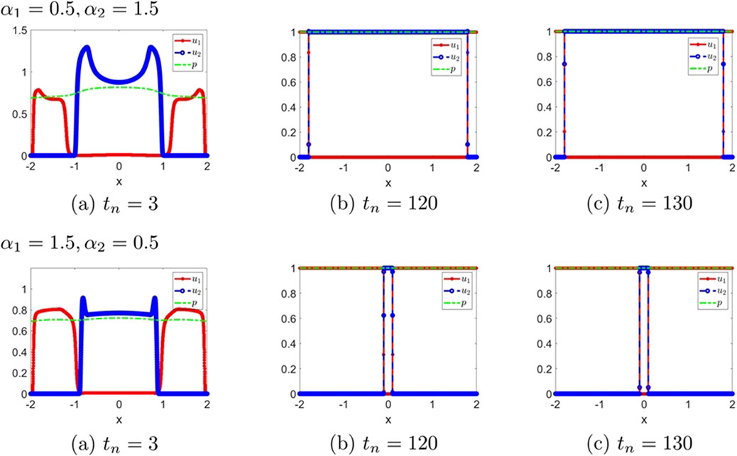
Figure 6. The numerical solution (Examples 1-2-8, 1-2-9). (a–c) show the evaluation of the numerical solution at different times.

Table 3

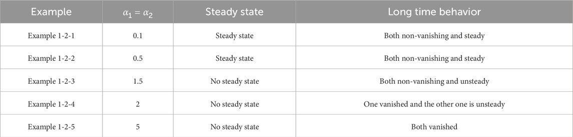
Table 3. Classification of asymptotic behavior $({\alpha }_1={\alpha }_2)$.

Table 4

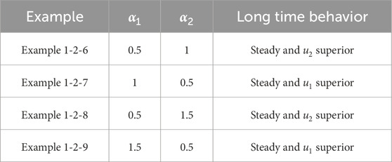
Table 4. Classification of asymptotic behavior $({\alpha }_1\ne {\alpha }_2)$.

3.2 Example 2 (segregated initial functions)

Set $I=[\mathrm{0,1}]$, $\chi =1$, $d_1=1$, $d_2=1$, and

$\begin{array}{cc}\hfill & h_{1,{\alpha }_1}\left(\left(u_1,u_2\right)\left(t,x\right)\right)=2-u_1\left(t-{\alpha }_1,x\right)-u_2\left(t,x\right),\hfill \\ \hfill & h_{2,{\alpha }_2}\left(\left(u_1,u_2\right)\left(t,x\right)\right)=2-u_1\left(t,x\right)-u_2\left(t-{\alpha }_2,x\right).\hfill \end{array}$

The initial conditions are set to

$\begin{array}{cc}\hfill & \begin{array}{c}\hfill u_1\left(t,x\right)=\left\{\begin{array}{cccc}\hfill & -10x\left(x-0.3\right)\hfill & \hfill & 0\le x\le 0.3\hfill \\ \hfill & 0\hfill & \hfill & \text{otherwise}\hfill \end{array}\right.\text{for\hspace{0.17em}all\hspace{0.17em}}t\le 0,\end{array}\hfill \\ \hfill & \begin{array}{c}\hfill u_2\left(t,x\right)=\left\{\begin{array}{cccc}\hfill & -10\left(1-x\right)\left(0.7-x\right)\hfill & \hfill & 0.7\le x\le 1\hfill \\ \hfill & 0\hfill & \hfill & \text{otherwise}\hfill \end{array}\right.\text{for\hspace{0.17em}all\hspace{0.17em}}t\le 0.\end{array}\hfill \end{array}$

We consider the following settings.

1. the classical hyperbolic Keller–Segel system

$•$ Example 2-1: ${\alpha }_1={\alpha }_2=0$;

2. ${\alpha }_1={\alpha }_2$

$•$ Example 2-2-1: ${\alpha }_1={\alpha }_2=0.1$,

$•$ Example 2-2-2: ${\alpha }_1={\alpha }_2=0.5$,

$•$ Example 2-2-3: ${\alpha }_1={\alpha }_2=1$,

$•$ Example 2-2-4: ${\alpha }_1={\alpha }_2=1.5$,

$•$ Example 2-2-5: ${\alpha }_1={\alpha }_2=2$,

$•$ Example 2-2-6: ${\alpha }_1={\alpha }_2=2.5$;

3. ${\alpha }_1\ne {\alpha }_2$

$•$ Example 2-2-7: ${\alpha }_1=0.5,{\alpha }_2=1$,

$•$ Example 2-2-8: ${\alpha }_1=1,{\alpha }_2=0.5$.

We fix $\tau =\frac{1}{2000}$, take the numerical solution with $h=\frac{1}{2000}$ at $T=1$ as the reference solution, and compute the errors for mesh sizes $h=\frac{1}{80},\frac{1}{160},\frac{1}{320},\frac{1}{640}$. The experimental errors for ${\alpha }_1={\alpha }_2=0$ and ${\alpha }_1={\alpha }_2=0.5$, shown in Tables 5, 6, respectively, indicate first-order convergence with respect to the mesh size $h$ for $\Vert u_{j,ref}^N-u_{j,h}^N{\Vert }_{L^2(I),{\mathcal{V}}_h}$ $(j=\mathrm{1,2})$ and $\Vert p_{\mathit{ref}}^N-p_h^N{\Vert }_{H^1(I),{\mathcal{V}}_h}$.

Table 5

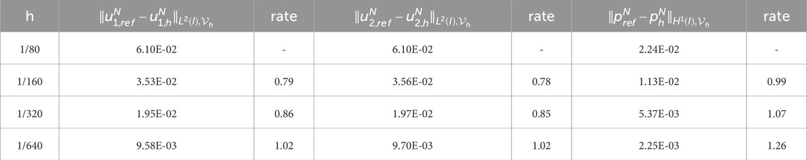
Table 5. Experimental errors and convergence order of $h$ for ${\alpha }_1={\alpha }_2=0$ (Example 2-1).

Table 6

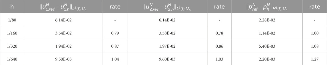
Table 6. Experimental errors and convergence order of $h$ for ${\alpha }_1={\alpha }_2=0.5$ (Example 2-2-2).

Figure 7 displays the evolution of solutions for the classical Keller–Segel system with $h=\tau =\frac{1}{2000}$. Figures 8–10 illustrate the dynamic behavior of the time-delayed nonlocal advection model with $h=\tau =\frac{1}{1000}$. Tables 7, 8 summarize the dynamic behaviors corresponding to the cases ${\alpha }_1={\alpha }_2$ and ${\alpha }_1\ne {\alpha }_2$, respectively. Symmetric delays in segregated initial functions, where the coefficients for $h_{1,{\alpha }_1}$ and $h_{2,{\alpha }_2}$ are the same, demonstrate that small delays $({\alpha }_1={\alpha }_2\le 0.5)$ can support steady coexistence. However, larger delays $({\alpha }_1={\alpha }_2\ge 1)$ may result in unsteady states or extinction. In Figure 10, we consider the case where ${\alpha }_1\ne {\alpha }_2$, revealing that the species with the larger delay often gain a competitive advantage.

Figure 7

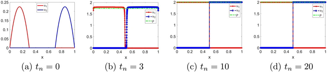
Figure 7. The numerical solution for ${\alpha }_1={\alpha }_2=0$ (Example 2-1). (a–d) show the evaluation of the numerical solution at different times.

Figure 8

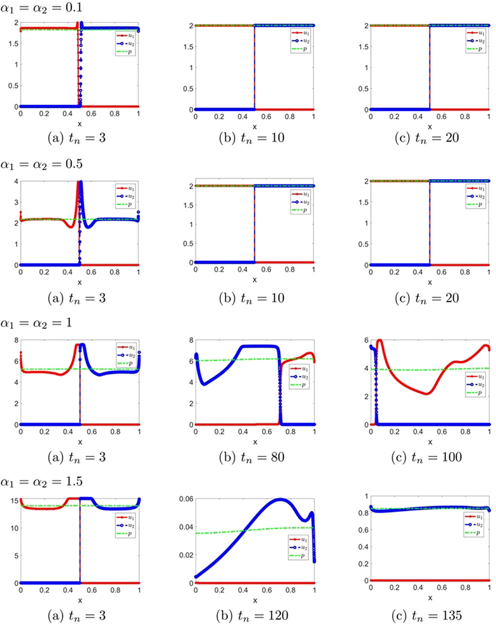
Figure 8. The numerical solution (Examples 2-2-1 through 2-2-4). (a–c) show the evaluation of the numerical solution at different times.

Figure 9

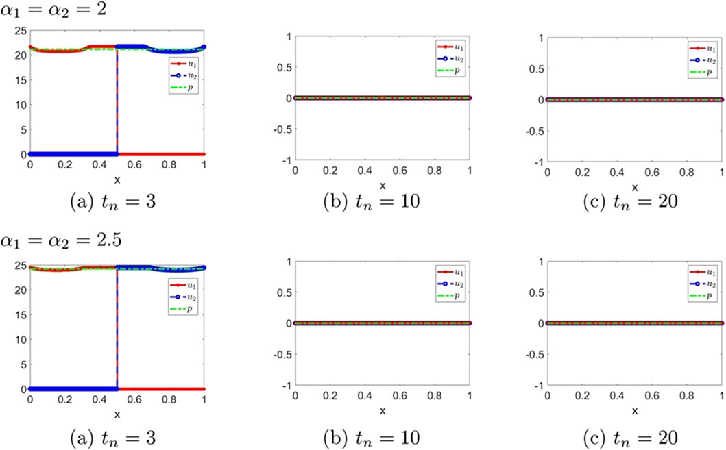
Figure 9. The numerical solution (Examples 2-2-5, 2-2-6). (a–c) show the evaluation of the numerical solution at different times.

Figure 10

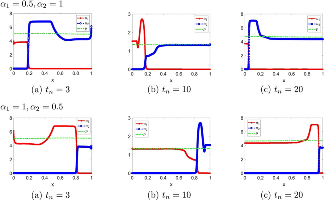
Figure 10. The numerical solution (Examples 2-2-7, 2-2-8). (a–c) show the evaluation of the numerical solution at different times.

Table 7

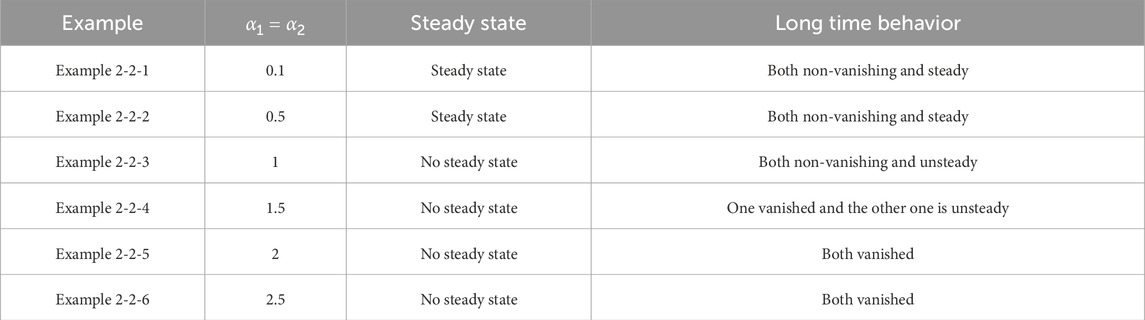
Table 7. Classification of asymptotic behavior $({\alpha }_1={\alpha }_2)$.

Table 8

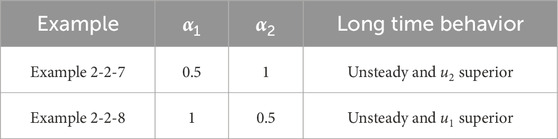
Table 8. Classification of asymptotic behavior $({\alpha }_1\ne {\alpha }_2)$.

3.3 Example 3 (segregated initial functions)

The settings are the same as those in Example 2, except that we choose

$\begin{array}{cc}\hfill & h_{1,{\alpha }_1}\left(\left(u_1,u_2\right)\left(t,x\right)\right)=2-2u_1\left(t-{\alpha }_1,x\right)-2u_2\left(t,x\right),\hfill \\ \hfill & h_{2,{\alpha }_2}\left(\left(u_1,u_2\right)\left(t,x\right)\right)=2-u_1\left(t,x\right)-u_2\left(t-{\alpha }_2,x\right).\hfill \end{array}$

The following parameters are considered.

1. the classical hyperbolic Keller–Segel system

$•$ Example 3-1: ${\alpha }_1={\alpha }_2=0$;

2. ${\alpha }_1={\alpha }_2$

$•$ Example 3-2-1: ${\alpha }_1={\alpha }_2=0.1$,

$•$ Example 3-2-2: ${\alpha }_1={\alpha }_2=0.5$,

$•$ Example 3-2-3: ${\alpha }_1={\alpha }_2=1$,

$•$ Example 3-2-4: ${\alpha }_1={\alpha }_2=4$;

3. ${\alpha }_1\ne {\alpha }_2$

$•$ Example 3-2-5: ${\alpha }_1=0.5,{\alpha }_2=1$,

$•$ Example 3-2-6: ${\alpha }_1=1,{\alpha }_2=0.5$.

We fix $\tau =\frac{1}{2000}$, take the numerical solution with $h=\frac{1}{2000}$ at $T=1$ as the reference solution, and compute the errors for mesh sizes $h=\frac{1}{80},\frac{1}{160},\frac{1}{320},\frac{1}{640}$. First-order convergence with respect to the mesh size $h$ is observed for $\Vert u_{j,ref}^N-u_{j,h}^N{\Vert }_{L^2(I),{\mathcal{V}}_h}$ $(j=\mathrm{1,2})$ and $\Vert p_{\mathit{ref}}^N-p_h^N{\Vert }_{H^1(I),{\mathcal{V}}_h}$, as shown in Table 9 for ${\alpha }_1={\alpha }_2=0$, and Table 10 for ${\alpha }_1={\alpha }_2=0.5$.

Table 9

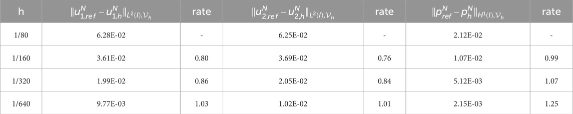
Table 9. Experimental errors and convergence order of $h$ for ${\alpha }_1={\alpha }_2=0$ (Example 3-1).

Table 10

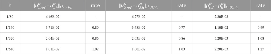
Table 10. Experimental errors and convergence order of $h$ for ${\alpha }_1={\alpha }_2=0.5$ (Example 3-2-2).

The evolutions of the solution for the classical Keller–Segel system $(h=\tau =\frac{1}{5000})$ are shown in Figure 11. Figures 12, 13 present the evolutions of the solution for the nonlocal advection model with time delays $(h=\tau =\frac{1}{5000})$. The dynamic behaviors for ${\alpha }_1={\alpha }_2$ and ${\alpha }_1\ne {\alpha }_2$ are summarized in Tables 11, 12, respectively. For the symmetric delays in the segregated initial functions, where the coefficients for $h_{1,{\alpha }_1}$ and $h_{2,{\alpha }_2}$ differ, small delays $({\alpha }_1={\alpha }_2\le 0.5)$ still result in the steady state (see Example 3-2-1 – Example 3-2-2, Figure 12). On the other hand, larger delays $({\alpha }_1={\alpha }_2\ge 1)$ can lead to unsteady dynamics and extinction (see Example 3-2-3 – Example 3-2-4, Figure 12). For the case with asymmetric delays, we see that both two examples are $u_2$ superior (see Example 3-2-5 – Example 3-2-6, Figure 13).

Figure 11

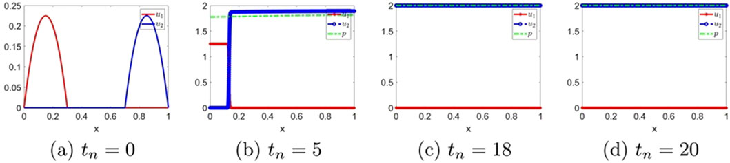
Figure 11. The numerical solution for ${\alpha }_1={\alpha }_2=0$ (Example 3-1). (a–d) show the evaluation of the numerical solution at different times.

Figure 12

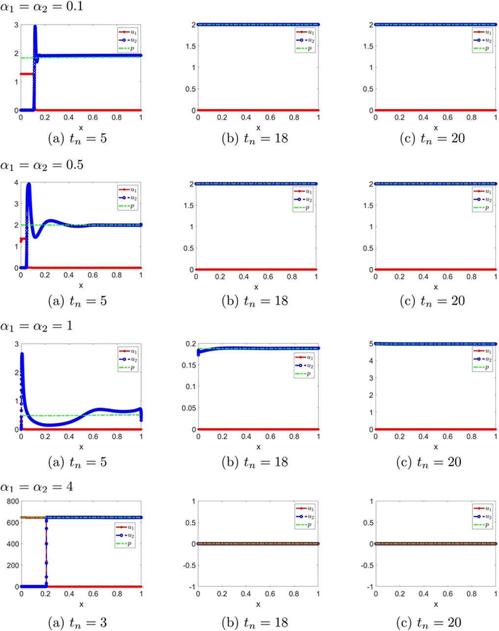
Figure 12. The numerical solution (Examples 3-2-1 through 3-2-4). (a–c) show the evaluation of the numerical solution at different times.

Figure 13

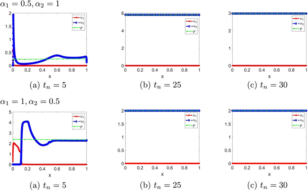
Figure 13. The numerical solution (Examples 3-2-5, 3-2-6). (a–c) show the evaluation of the numerical solution at different times.

Table 11

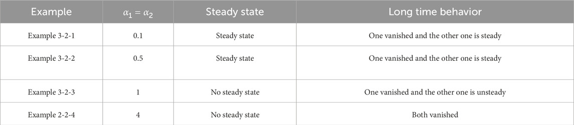
Table 11. Classification of asymptotic behavior $({\alpha }_1={\alpha }_2)$.

Table 12

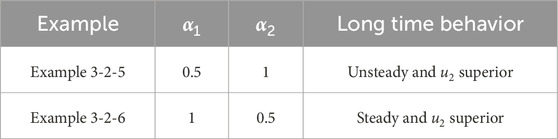
Table 12. Classification of asymptotic behavior $({\alpha }_1\ne {\alpha }_2)$.

Remark 3.1. We observe that small symmetric delays $({\alpha }_1={\alpha }_2)$ result in the steady state. This suggests that ecosystems with balanced feedback mechanisms (e.g., similar resource recovery times for competing species) are more likely to maintain biodiversity. On the other hand, larger symmetric delays $({\alpha }_1={\alpha }_2)$ can lead to unsteady dynamics and extinction, which align with scenarios where delayed interventions (e.g., pesticide application or vaccination campaigns) fail to prevent population collapse. Moreover, asymmetric delay parameters $({\alpha }_1\ne {\alpha }_2)$ between the two species tend to confer a competitive advantage to one species. Such dynamics are relevant in tumor-microenvironment interactions, where targeting delay mechanisms could alter competitive outcomes.

4 Conclusion

This study proposes a nonlocal advection model with time delays to investigate the population dynamics of two competing species, extending previous frameworks by incorporating delayed interactions between migration and resource recovery. A positivity-preserving finite volume scheme is developed to ensure biologically realistic solutions. Numerical experiments demonstrate that small symmetric delays $({\alpha }_1={\alpha }_2)$ are steady, while larger delays induce unsteady states and potential extinction of one or both species. Moreover, asymmetric delay parameters between the two species tend to confer a competitive advantage to one species. Future work may explore applications to more complex ecological systems, incorporate stochastic or spatially heterogeneous delays, and extend the model to multi-species interactions or adaptive delay mechanisms for deeper insights into delayed feedback effects in biological processes. As a future work, we would like to consider the development of high-dimensional chemotaxis models with time delays, explore alternative numerical schemes to improve computational efficiency, and ensure that the system properties (such as positivity preservation, conservation laws, and energy dissipation) are maintained.

Data availability statement

The original contributions presented in the study are included in the article/supplementary material, further inquiries can be directed to the corresponding author.

Author contributions

PZ: Writing – original draft, Data curation, Writing – review and editing, Methodology. YE: Writing – review and editing, Funding acquisition, Supervision, Methodology. GZ: Funding acquisition, Methodology, Supervision, Investigation, Writing – review and editing.

Funding

The author(s) declare that financial support was received for the research and/or publication of this article. This work was supported by JSPS KAKENHI Grant Number 25K07137, NSFC General Project No. 12171071, and the Natural Science Foundation of Sichuan Province No. 2023NSFSC0055.

Conflict of interest

The authors declare that the research was conducted in the absence of any commercial or financial relationships that could be construed as a potential conflict of interest.

Generative AI statement

The author(s) declare that no Generative AI was used in the creation of this manuscript.

Any alternative text (alt text) provided alongside figures in this article has been generated by Frontiers with the support of artificial intelligence and reasonable efforts have been made to ensure accuracy, including review by the authors wherever possible. If you identify any issues, please contact us.

Publisher’s note

All claims expressed in this article are solely those of the authors and do not necessarily represent those of their affiliated organizations, or those of the publisher, the editors and the reviewers. Any product that may be evaluated in this article, or claim that may be made by its manufacturer, is not guaranteed or endorsed by the publisher.

References

1. Murray JD. Spatial models and biomedical applications. New York: Springer (2003).

Google Scholar

2. Murray JD. Mathematical biology I. An introduction, 17. Berlin: Springer (2007).

Google Scholar

3. Pasquier J, Galas L, Boulangé-Lecomte C, Rioult D, Bultelle F, Magal P. Different modalities of intercellular membrane exchanges mediate cell-to-cell p-glycoprotein transfers in MCF-7 breast cancer cells. J Biol Chem (2012) 287(10):7374–87. doi:10.1074/jbc.M111.312157

PubMed Abstract | CrossRef Full Text | Google Scholar

4. Lou Y, Ni W. Diffusion, self-diffusion and cross-diffusion. J Differ Equ (1996) 131(1):79–131. doi:10.1006/jdeq.1996.0157

CrossRef Full Text | Google Scholar

5. Lou Y, Ni W. Diffusion vs cross-diffusion: an elliptic approach. J Differ Equ (1999) 154(1):157–90. doi:10.1006/jdeq.1998.3559

CrossRef Full Text | Google Scholar

6. Shigesada N, Kawasaki K, Teramoto E. Spatial segregation of interacting species. J Theor Biol (1979) 79(1):83–99. doi:10.1016/0022-5193(79)90258-3

PubMed Abstract | CrossRef Full Text | Google Scholar

7. Fu X, Griette Q, Magal P. A cell-cell repulsion model on a hyperbolic Keller–Segel equation. J Math Biol (2020) 80(7):2257–300. doi:10.1007/s00285-020-01495-w

PubMed Abstract | CrossRef Full Text | Google Scholar

8. Fu X, Magal P. Asymptotic behavior of a nonlocal advection system with two populations. J Dyn Differ Equ (2022) 34(3):2035–77. doi:10.1007/s10884-021-09956-6

CrossRef Full Text | Google Scholar

9. Horstmann D. From 1970 until present: the Keller–Segel model in chemotaxis and its consequences. Jahresber Dtsch Math.-Ver (2003) 195(1):103–65. Available online at: https://cir.nii.ac.jp/crid/1571698600200464128

Google Scholar

10. Horstmann D. From 1970 until present: the Keller–Segel model in chemotaxis and its consequences. Jahresber Dtsch Math.-Ver (2004) 106:51–69. Available online at: https://cir.nii.ac.jp/crid/1570291226041248512

Google Scholar

11. Keller EF, Segel LA. Model for chemotaxis. J Theor Biol (1971) 30(2):225–34. doi:10.1016/0022-5193(71)90050-6

PubMed Abstract | CrossRef Full Text | Google Scholar

12. Patlak CS. Random walk with persistence and external bias. Bull Math Biophys (1953) 15:311–38. doi:10.1007/bf02476407

CrossRef Full Text | Google Scholar

13. Fu X, Griette Q, Magal P. Existence and uniqueness of solutions for a hyperbolic Keller–Segel equation, Discrete Contin. Dyn Syst Ser B (2021) 26(4):1931–66. doi:10.3934/dcdsb.2020326

CrossRef Full Text | Google Scholar

14. Perthame B, Dalibard A. Existence of solutions of the hyperbolic Keller–Segel model. Trans Am Math Soc (2009) 361(5):2319–35. doi:10.1090/s0002-9947-08-04656-4

CrossRef Full Text | Google Scholar

15. Bruno L, Tosin A, Tricerri P, Venuti F. Non-local first-order modelling of crowd dynamics: a multidimensional framework with applications. Appl Math Model (2011) 35(1):426–45. doi:10.1016/j.apm.2010.07.007

CrossRef Full Text | Google Scholar

16. Colombo RM, Garavello M, Lécureux-Mercier M. A class of nonlocal models for pedestrian traffic. Math Models Methods Appl Sci (2012) 22(4):1150023. doi:10.1142/s0218202511500230

CrossRef Full Text | Google Scholar

17. Bürger R, Goatin P, Inzunza D, Villada LM. A non-local pedestrian flow model accounting for anisotropic interactions and domain boundaries. Math Biosci Eng (2020) 17(5):5883–906. doi:10.3934/mbe.2020314

PubMed Abstract | CrossRef Full Text | Google Scholar

18. Goatin P, Inzunza D, Villada LM. Numerical comparison of nonlocal macroscopic models of multi-population pedestrian flows with anisotropic kernel. Springer (2022). p. 371–81.

Google Scholar

19. Kuang Y. Delay differential equations. New York: Academic Press (1993).

Google Scholar

20. Smith HL. An introduction to delay differential equations with applications to the life sciences. New York: Springer (2011).

Google Scholar

21. Volterra V. Leçons sur la Théorie Mathématique de la Lutte pour la Vie. Paris: Gauthier-Villars (1931).

Google Scholar

22. Cushing JM. Time delays in single species growth models. J Math Biol (1977) 4(3):257–64. doi:10.1007/bf00280975

PubMed Abstract | CrossRef Full Text | Google Scholar

23. Cushing JM. Integrodifferential equations and delay models in population dynamics, 20. Berlin: Springer (2013).

Google Scholar

24. Miller RK. On Volterra’s population equation. SIAM J Appl Math (1966) 14(3):446–52. doi:10.1137/0114039

CrossRef Full Text | Google Scholar

25. Bownds JM, Cushing JM. On the behavior of solutions of predator-prey equations with hereditary terms. Math Biosci (1975) 26(1-2):41–54. doi:10.1016/0025-5564(75)90093-0

CrossRef Full Text | Google Scholar

26. Macdonald N. Time delay in prey-predator models. Math Biosci (1976) 28(3-4):321–30. doi:10.1016/0025-5564(76)90130-9

CrossRef Full Text | Google Scholar

27. Gopalsamy K, Aggarwala BD. Limit cycles in two spacies competition with time delays. J Austral Math Soc (1980) 22(2):148–60. doi:10.1017/s033427000000223x

CrossRef Full Text | Google Scholar

28. Shibata A, Saitô N. Time delays and chaos in two competing species. Math Biosci (1980) 51(3-4):199–211. doi:10.1016/0025-5564(80)90099-1

CrossRef Full Text | Google Scholar

29. Saito N. Conservative upwind finite-element method for a simplified Keller–Segel system modelling chemotaxis. IMA J Numer Anal (2007) 27(2):332–65. doi:10.1093/imanum/drl018

CrossRef Full Text | Google Scholar

30. Saito N. Error analysis of a conservative finite-element approximation for the Keller–Segel system of chemotaxis. Commun Pure Appl Anal (2011) 11(1):339–64. doi:10.3934/cpaa.2012.11.339

CrossRef Full Text | Google Scholar

31. Saito N, Suzuki T. A finite difference scheme to the system of self-interacting particles. RIMS Kôkyûroku (2003) 1320:18–28. Available online at: http://hdl.handle.net/2433/43075

Google Scholar

32. Saito N, Suzuki T. Notes on finite difference schemes to a parabolic-elliptic system modelling chemotaxis. Appl Math Comput (2005) 171(1):72–90. doi:10.1016/j.amc.2005.01.037

CrossRef Full Text | Google Scholar

33. Zhou G, Saito N. Finite volume methods for a Keller–Segel system: discrete energy, error estimates and numerical blow-up analysis. Numer Math (2017) 135(1):265–311. doi:10.1007/s00211-016-0793-2

CrossRef Full Text | Google Scholar

34. Cross L, Zhang X. On the monotonicity of Q²spectral element method for Laplacian on quasi-uniform rectangular meshes. Commun Comput Phys (2024) 35(1):60–180. doi:10.4208/cicp.oa-2023-0206

CrossRef Full Text | Google Scholar

35. Zhang X, Shu C. On maximum-principle-satisfying high order schemes for scalar conservation laws. J Comput Phys (2010) 229(9):3091–120. doi:10.1016/j.jcp.2009.12.030

CrossRef Full Text | Google Scholar

36. Zhang X, Shu C. Maximum-principle-satisfying and positivity-preserving high-order schemes for conservation laws: survey and new developments. P Roy Soc A.-math Phy (2011) 467(2134):2752–76. doi:10.1098/rspa.2011.0153

CrossRef Full Text | Google Scholar