High-precision shape reconstruction for optical fiber sensors based on cubic spline interpolation and tangent angle recursion

Accurate reconstruction of optical fiber curves has important applications in fields like medicine, aerospace, and infrastructure monitoring. However, it faces challenges such as insufficient reconstruction accuracy. In this paper, a novel method for optical fiber plane curve reconstruction, based on cubic spline interpolation and the tangent angle recursion algorithm, is proposed. First, the optical fiber sensor demodulation system is utilized to acquire strain information on the surface of the flexible substrate. Then, based on the approximate relationship between wavelength and curvature, discrete curvature values are calculated from experimental data. Next, the cubic spline interpolation is applied to convert the discrete curvature into a continuous profile, ensuring the smoothness of the curve. Finally, the tangent-angle recursive algorithm is employed to derive the coordinates of arbitrary points on the fiber deformation curve, thereby realizing precise reconstruction of the optical fiber curve. Additionally, the Frenet-Serret framework is introduced, which can be employed for 3D reconstruction, and a sensitivity analysis of the key parameters is conducted, exploring the impact of the number of sampling and interpolation points on the reconstruction accuracy. The reconstruction results show that the curves have a high degree of smoothness and physical realism. With 50 sampling points and no interpolation, the mean absolute error (MAE) reaches 0.000892 m, approximately 72% lower than with 20 sampling points and no interpolation. The root mean square error (RMSE) is 0.001127 m, about 75% lower than with 20 sampling points and no interpolation, thereby verifying the feasibility of the method. This study offers theoretical foundations and experimental validation for the optimization of optical fiber shape sensing technology, thus holding significant importance for enhancing measurement accuracy and advancing engineering applications in related domains.

1 Introduction

Optical fiber sensing is an advanced sensing technology developed in the 1970s along with optical fiber and optical communication technologies [1–3]. It uses light waves as the sensing signal and optical fiber as the transmission medium to detect signals from the external environment. The basic principle is that changes in external environmental parameters, such as temperature and pressure, give rise to corresponding variations in the optical fiber’s light wave parameters (e.g., wavelength, phase, intensity). In other words, external signals modulate the optical signals. The structure of the optical fiber is shown in Figure 1a and the propagation of light within the fiber is illustrated in Figure 1b. In recent years, with the continuous development of optical fiber sensing technology, optical fibers have demonstrated significant potential in the field of shape measurement. In the medical field [4, 5], optical fiber shape sensing has been successfully applied to real-time monitoring of endoscopic catheters and robotic surgical instruments, offering sub-millimeter spatial resolution and accurate 3D morphology reconstruction [6, 7]. This significantly enhances the safety and accuracy of minimally invasive surgeries. In the aerospace sector [8–10], optical fiber shape sensing systems are employed to monitor the deformation of critical structures such as wings and fuselages, providing crucial support for flight safety. In the field of infrastructure [11–13], this technology enables distributed shape monitoring of structures such as pipelines, bridges, tunnels, thereby helping to prevent structural failures and accidents.

Figure 1

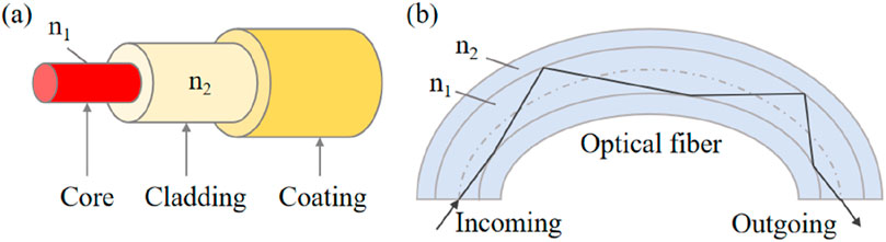
Figure 1. (a) Fiber structure diagram; (b) Transmission of light waves in optical fibers.

With the gradual maturity of optical fiber technology, it is necessary to study its shape sensing algorithms. Among the many optical fiber reconstruction methods, researchers primarily employ the strain-geometry mapping principle to achieve shape reconstruction through various mathematical models. For example, Pauer et al [14] consider the measurement unit system as a sensor network, where data collected by sensors randomly distributed over the fiber are processed by specific algorithms, ultimately enabling the reconstruction of the spatial shape of the fiber. Khan et al. [15] transformed data from FBG sensors into strain measurements, which were subsequently used to calculate the curvature and torsion of the fiber. By integrating the Frenet-Serret equations with the calculated curvature and torsion, they reconstructed the shape of the instrument. Lv et al. [16] proposed a 3D shape reconstruction method for multicore optical fibers based on curvature and angle correction. This method improves the reconstruction algorithm for flexible, 3D-deformed multicore optical fiber by introducing directional angle and curvature correction coefficients. Souza et al. [17] integrated five distributed FBG sensors along a pinus wood beam and a nylon 6.0 beam. The sensors estimated the elastic line describing the deflection over the entire length of the beam by replicating load application tests. Ferreira et al. [18] evaluated the curvature of a specific cross-section by installing a fiber Bragg grating sensor on the beam, then reconstructed the deformation profile by integration.

However, in the field of optical fiber curve reconstruction, classical algorithms still face several limitations. Cubic spline interpolation can effectively ensure smooth curvature distribution, but it is sensitive to experimental noise and prone to error propagation. The tangent angle recursion algorithm can reconstruct a plane curve from curvature information, yet it is susceptible to error accumulation over long reconstruction distances (see Table 1). In summary, although these methods have been verified in theory and practice, optimizing their combination and reducing errors in practical implementation remain critical challenges. To address these issues, this paper proposes a hybrid reconstruction algorithm integrating cubic spline interpolation and tangent angle recursion algorithm. Specifically, a strain-wavelength-curvature closed-loop model is constructed using MATLAB. This model provides an improved solution for optical fiber shape sensing by establishing a systematic mapping from strain measurements to geometric curvature through wavelength-dependent relationships (see Figure 2).

Table 1

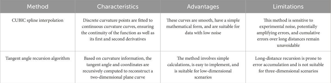
Table 1. Comparison of different fiber shape reconstruction methods.

Figure 2

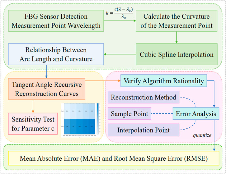
Figure 2. Flowchart of optical fiber sensor curvature reconstruction and error analysis methodology.

2 Curve reconstruction methods

2.1 Calculation of curves

In order to facilitate the wavelength measurement, the coordinates of the initial point are set as the origin, with the initial horizontal fiber direction as the x-axis, and the vertical direction as the y-axis. After force is applied in the plane, the tangent of the fiber at the initial position forms a 45° angle with the horizontal direction. FBG sensors were used for the measurements, with a spacing of 0.6 m between them (see Figure 3). The wavelength of the signal at each sensor position was first measured when the fiber is horizontal, and then measured again after the fiber is subjected to an external force. The fiber Bragg grating (FBG) sensors employed in this study had a grating length of 10 mm, providing sufficient resolution for detecting wavelength shifts while ensuring stable reflection characteristics.

Figure 3

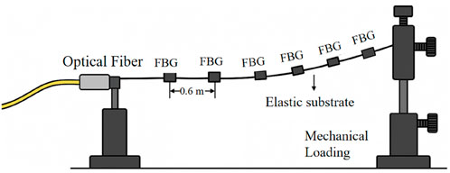
Figure 3. Schematic diagram of the experimental setup used for measurement.

In this setup, the optical fiber is attached to a flexible polycarbonate beam serving as the elastic substrate, while mechanical loading is applied through a bending device with adjustable weights. When the loading device induces bending in the substrate, the FBG region undergoes stretching or compression along with the fiber, thereby enabling the detection of local axial strain at that specific location.

The optical fiber sensor demodulation system extracts strain information, which is then used to indirectly determine the curvature. Given the relationship between curvature and strain, the relationship can be expressed as Equation 1 [19]:

$\epsilon =\frac{h}{2}·k(1)$

where $h$ denotes the distance between each test point and the neutral axis, and $k$ represents curvature. Based on the relationship between the central wavelength shift and the strain [19], the curvature can be expressed approximately as follows:

$k=\frac{c\left(\lambda -{\lambda }_0\right)}{{\lambda }_0}(2)$

where ${\lambda }_0$ is the wavelength measured in the initial state of the horizontal fiber. $\lambda$ is the wavelength measured after the fiber is subjected to an external force. $c$ is a constant (4,200 m^-1) that represents a scale factor obtained via experimental calibration. In this experiment, the wavelength values before and after loading were measured for two different initial states, and the results are presented in Table 2. The wavelength data in Table 2 were obtained using a Yokogawa AQ6370D spectrum analyzer, which has a resolution bandwidth of 0.02 nm.

Table 2

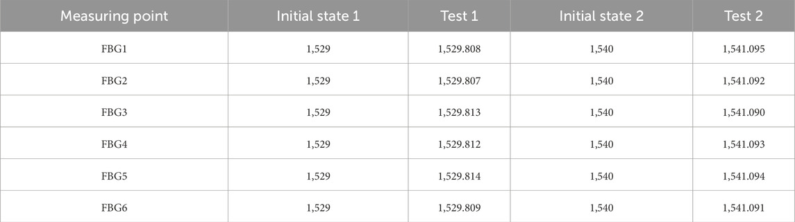
Table 2. Wavelength (nm) measurement data.

2.2 Cubic spline interpolation

Cubic spline interpolation [20–22] is a piecewise interpolation method. It divides the interpolation interval into subintervals and generates a polynomial of degree at most three for each subinterval. These polynomials are constructed to satisfy continuity of the function itself as well as its first and second derivatives, ensuring smoothness and continuity at every point.

Splitting the fiber into $n$ segments on average, i.e., there exist $n+1$ splitting points satisfying $S_1<S_2<\dots <S_{\mathrm{n}+1}$, where $S_i$ is the distance of a point on the fiber from the starting point, then the curvature satisfies the functional relationship given in Equation 3 with the length of the fiber on the corresponding interval $\left[S_i,S_{i+1}\right],\left(i=1,2,\dots ,n\right)$:

$k\left(S\right)=a_i+b_i\times \left(S-S_i\right)+c_i\times {\left(S-S_i\right)}^2+d_i\times {\left(S-S_i\right)}^3(3)$

where: $a_i$, $b_i$, $c_i{d}_i$ are 4 coefficients to be determined. The curve satisfies the following relationship at the $i$ th split point:

$\left\{\begin{array}{l}{k}_i\left(S_i\right)=C_i\\ k_i\left(S_{i+1}\right)=C_{i+1}\\ {k_i}^{\prime }\left(S_{i+1}\right)={k_{i+1}}^{\prime }\left(S_{i+1}\right)\\ {k_i}^{″}\left(S_{i+1}\right)={k_{i+1}}^{″}\left(S_{i+1}\right)\end{array}\right.(4)$

That is, the curvature satisfies the interpolating continuity condition, as well as the continuity of the first and second derivatives. This ensures that the fitted curvature curve is smooth. Equation 4, together with the boundary constraints at the beginning and end of the curve, can be used to determine the four coefficients. Here the natural boundary conditions are used as Equation 5:

$\left\{\begin{array}{l}{k}^{″}\left(0\right)=0\\ k^{″}\left(S_{total}\right)=0\end{array}\right.(5)$

2.3 Tangent angle recursion algorithm

As the experiments are conducted on the surface of a flexible substrate for monitoring, this study focuses on the deformation of the optical fiber caused by a force applied in a single plane, without considering torsional changes of the fiber in three-dimensional space. It is suitable for low-dimensional application scenarios, such as flexible substrate surface monitoring and simplified preliminary validation, where torsional effects are minimal.

Based on the derived curvature and the initial condition that the tangent line at the initial position of the fiber forms a 45 $°$ angle with the horizontal after planar stress is applied, the tangent angle recursion algorithm [23–25] is employed to obtain the coordinates of any point on the fiber deformation curve, thereby enabling the reconstruction of the curve.

For curves, the arc between two points on a curve can be approximated as a segment of a microcircular arc, provided the points are sufficiently close together. Let the curvature of the curve segment between the starting point $O_n$ and the end point$O_{n+1}$ be $k_n$ and $k_{n+1}$, respectively. The corresponding coordinates of these points are $\left(x_n,y_n\right)$ and $\left(x_{n+1},y_{n+1}\right)$, respectively. ${\beta }_n$ and ${\beta }_{n+1}$ are the angles between the tangent lines and the x-direction of the two places $O_n$ and $O_{n+1}$, respectively. The angle of the center of the circle corresponding to the arc can be expressed as Equation 6:

$\Delta {\alpha }_n={\beta }_{n+1}-{\beta }_n(6)$

The chord length $l_n$ of an arc can be expressed as Equation 7:

$\left\{\begin{array}{l}{l}_n=2\sin \left(\frac{\Delta {\alpha }_n}{2}\right)/k_n=2\sin c\left(\frac{\Delta {\alpha }_n}{2}\right)·\frac{\Delta {\alpha }_n}{k_n},\left(k_n\ne 0\right)\\ l_n=\Delta s,\left(k_n=0\right)\end{array}\right.(7)$

where $k_n$ is the curvature corresponding to the arc. The coordinate increment$\left(\Delta x_n,\Delta y_n\right)$ is calculated from the chord length using Equation 8:

$\left\{\begin{array}{l}\Delta x=l_n·\cos \left({\alpha }_n-\Delta {\alpha }_n/2\right)\\ \Delta y=l_n·\sin \left({\alpha }_n-\Delta {\alpha }_n/2\right)\end{array}\right.(8)$

From the recurrence formula, the new coordinates can be expressed as Equation 9:

$\left\{\begin{array}{l}{x}_{n+1}=x_n+\Delta x\\ y_{n+1}=y_n+\Delta y\end{array}\right.(9)$

According to the definition of curvature from Equation 10:

$\beta \left(s\right)=\int k\left(s\right)ds(10)$

2.4 3D curve reconstruction and torsion compensation

The Frenet-Serret formulas constitute a system of differential equations that characterize the position and orientation of a curve in three-dimensional space [26]. These equations describe the curve’s geometry in terms of its curvature and torsion. At any point on a curve in three-dimensional space, the Frenet-Serret formulas use the tangent, normal, and binormal vectors to define a local orthonormal coordinate system moving along the curve. The translation of this coordinate system is described by Equation 11:

${\mathit{p}}_{i+1}={\left[\begin{array}{ccc}-\left(1-\cos \left({\theta }_i\right)\right)/k_i& 0& \sin \left({\theta }_i\right)/k_i\end{array}\right]}^T(11)$

The new coordinate system is subsequently rotated around the axis ${\theta }_i$ and ${∆\phi }_{i+1}$, resulting in two distinct rotation matrices as given in Equations 12, 13:

${\mathit{T}}_{B_i}^{{\theta }_i}=\left[\begin{array}{cccc}\cos \left({\theta }_i\right)& 0& -\sin \left({\theta }_i\right)& 0\\ 0& 1& 0& 0\\ \sin \left({\theta }_i\right)& 0& \cos \left({\theta }_i\right)& 0\\ 0& 0& 0& 1\end{array}\right](12)$

${\mathit{T}}_{T_i}^{\Delta \phi \omega 1}=\left[\begin{array}{cccc}\cos \left(\Delta {\phi }_{i+1}\right)& -\sin \left(\Delta {\phi }_{i+1}\right)& 0& 0\\ \sin \left(\Delta {\phi }_{i+1}\right)& \cos \left(\Delta {\phi }_{i+1}\right)& 0& 0\\ 0& 0& 1& 0\\ 0& 0& 0& 1\end{array}\right](13)$

Consequently, the constant transformation matrix enables the continuous construction of a moving coordinate system. At each step, the endpoint of each micro-segment is updated and connected, yielding the fitted curve.

3 Reconstruction results and discussion

3.1 Characteristics of reconstruction curve

After obtaining the wavelength information from each sensing point, the corresponding discrete curvature values from two tests were calculated using Equation 2, and the results are presented in Table 3.

Table 3

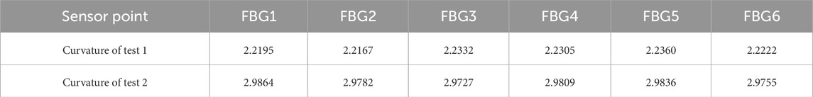
Table 3. Curvature (m^-1) of each sensing point after two tests.

Using the curvature values calculated at each sensing point and applying cubic spline interpolation, the curvature distributions of Test 1 and Test 2 along different arc lengths are shown in Figures 4a,b. These results demonstrate that cubic spline interpolation effectively fits the discrete curvature data measured by the fiber, with curvature values along the central axis in both Tests 1 and 2 ranging from 2 to 3. This provides a smooth and physically meaningful curvature distribution that serves as a reliable basis for subsequent curve reconstruction. Additionally, Figure 4b exhibits more pronounced curvature fluctuations compared to Figure 4a, suggesting that the initial state or loading conditions have a significant influence on the fiber’s deformation response.

Figure 4

Figure 4. Curvature distribution: (a) Test 1; (b) Test 2.

In the initial state, the optical fiber is aligned along the horizontal direction (x-axis), with the vertical direction as the y-axis. After deformation under the force, the tangent at the fiber’s initial point forms a 45° angle with the horizontal axis. Therefore, the initial coordinate of the deformation curve is $\left(x_0,y_0\right)=\left(0,0\right)$, and ${\beta }_0=45°$.

By using the curvature values at the endpoints of each arc segment obtained through cubic spline interpolation and applying the tangent angle recursion algorithm, the coordinates of any point on the fiber deformation curve can be derived. This enables the reconstruction of the curve, as shown in Figures 5a,b. It can be seen that the reconstructed curve exhibits an approximately circular shape. In Figure 5a, because the applied force is relatively small, the deformation pattern of the optical fiber remains simple and symmetric, leading to a clearly visible overlapping region. In contrast, the overlapping region in Figure 5b is larger than that in Figure 5a, as the force applied in Test 2 exceeds that in Test 1. Moreover, it can be anticipated that with further increases in the applied force, a spiral structure would emerge in the middle of the curve in a three-dimensional scenario. The geometry of the curves is governed by the curvature distribution. Regions of high curvature indicate a greater change in direction over shorter distances, suggesting stronger external forces in these regions. Conversely, regions of low curvature are closer to straight lines, reflecting either smaller external forces or the inherent properties of the material.

Figure 5

Figure 5. The reconfiguration curves: (a) Test 1; (b) Test 2.

The reconstructed curves are continuous and smooth, without sudden changes in direction. The smooth curve generated by cubic spline interpolation ensures the physical realism of the phenomenon. In optical fiber curve reconstruction, smoothness implies continuous force interactions and material responses along the fiber, preventing abrupt transitions and helping to avoid structural instabilities in practical applications.

3.2 Sensitivity analysis of the parameter $\mathit{c}$

The parameter $c$ is a calibration constant obtained experimentally, which establishes the relationship between the measured wavelength shift and the corresponding curvature. Although parameter$c$ remains constant within a given experiment, its value directly influences the magnitude of the calculated curvature. Therefore, to evaluate the robustness of the reconstruction method, a sensitivity analysis of parameter$c$ is conducted. Figure 6a illustrates that the Test 1 curve exhibits a relatively mild slope, with the average curvature displaying an approximately linear increase as the parameter $c$ increases. The sensitivity curve of Test 2 presents a lower slope than that of Test 1, and similarly follows a linear increasing pattern. When the parameter $c$ lies within the range of $\left[4000,4400\right]$, the curvature increases by approximately $\Delta k=0.3m^{-1}$, indicating a low level of sensitivity.

Figure 6

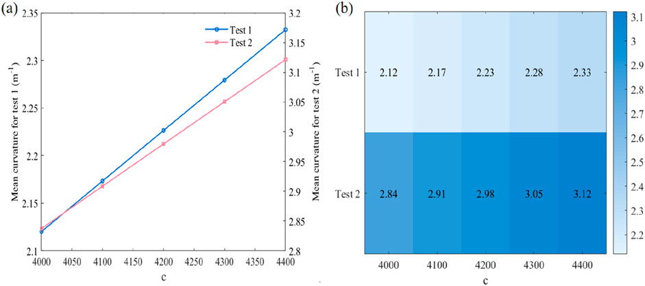
Figure 6. (a) Comparison of the effect of parameter $c$ on the mean curvature; (b) Heat maps for parameter $c$.

Figure 6b distinctly reveals the influence of the parameter $c$ on the mean curvature response of the optical fiber sensor. The horizontal axis represents the values of the parameter$c$ (ranging from 4,000 to 4,400 in increments of 100), while the vertical axis distinguishes between the two initial conditions of Test 1 and Test 2. Additionally, Test 2 exhibits a generally darker hue, indicating that its mean curvature values are consistently higher than those of Test 1. This reflects the differing system responses under varying initial wavelength conditions. Both bands exhibit a progressive shift from lighter to darker tones with increasing parameter values. However, the more pronounced gradient observed in Test 2 indicates that the system with an initial wavelength of 1,540 nm exhibits enhanced sensitivity to parameter variations. Notably, both color bands are situated within the mid-tone region. This offers a valuable reference for parameter calibration in practical engineering applications. These results not only verify the critical role of the parameter $c$, but also provide a visual framework for the optimization of the sensor and the management of associated errors in subsequent stages.

3.3 Validation of the reconfiguration method

Based on the plane curve equation $y=x^3+x\left(0\le x\le 1\right)$, points are sampled at appropriately spaced arc lengths. The curvature at each sampled point is then calculated. These curvature values serve as the foundation for reconstructing the plane curve via a tangent angle recursion algorithm. The reconstructed curves are compared with the originals to verify the feasibility of the method and to analyze the sources of discrepancies.

3.3.1 Calculation of arc length and curvature

For a given curve $y=x^3+x\left(0\le x\le 1\right)$, first calculate the differential $dy/dx$ as Equation 14:

$\frac{dy}{dx}=3x^2+1(14)$

Then the differential $ds$ of the arc length is [27] as Equation 15:

$ds=\sqrt{1+{\left(\frac{dy}{dx}\right)}^2}=\sqrt{1+{\left(3x^2+1\right)}^2}dx(15)$

The arc length is then obtained by integration as Equation 16:

$s={\int }_0^1\sqrt{1+{\left(3x^2+1\right)}^2}dx(16)$

The value of curvature as a function of arc length is determined by the curvature formula given in Equation 17:

$k=\frac{\left|y^{″}\right|}{{\left(1+y{\prime }^2\right)}^{\frac{3}{2}}}(17)$

Where $y^{\prime }=\frac{dy}{dx}$, $y^{″}=\frac{d^{2}y}{d{x}^2}$.

Taking into account the range of $x$ and computational complexity, 20 sampling points are selected along equally spaced arc lengths from the origin, covering the range $x=0$ to $x=1$.

3.3.2 Comparison of reconstruction curves

The reconstructed curves derived from the tangent angle recursion algorithm are compared with the original curves for sample sizes of 20 and 50 without interpolation, as shown in Figures 7a,b respectively. The results show that increasing the number of sampling points improves alignment accuracy: the reconstructed curve in Figure 7b matches the original curve more closely than in Figure 7a. With an initial sampling size of 20, cubic spline interpolation is employed to increase the number of points to 50 and 100. The reconstructed curves generated via the tangent angle recursion method are subsequently compared with the original curves, as presented in Figures 8a,b respectively. When interpolated to 50 and 100 points, the reconstructed curves closely align with the original curves. Notably, the agreement is further improved at 100 interpolation points, demonstrating a more precise match.

Figure 7

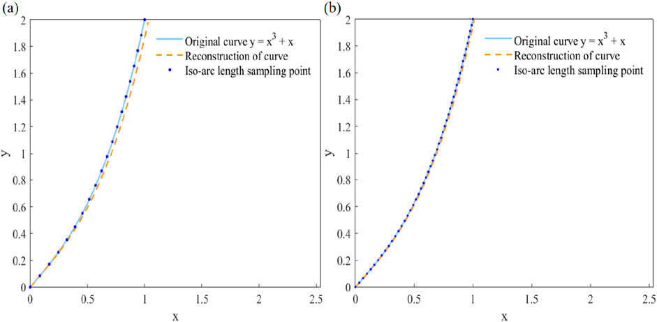
Figure 7. Comparison of original and reconstructed curves: (a) The sampling point is 20; (b) The sampling point is 50.

Figure 8

Figure 8. Comparison of original and reconstructed curves: (a) Add to 50 interpolation points; (b) Add to 100 interpolation points.

3.3.3 Error analysis

A comprehensive analysis of the errors in the fiber reconstruction process reveals three main contributing factors. First, the sampling interval and the number of sampling points significantly influence the accuracy of the reconstructed curve. Second, with fixed sampling points, the interpolation of curvature data affects the reconstruction results. Finally, the choice of reconstruction algorithm also impacts the final curve. Alternative fiber reconstruction algorithms are beyond the scope of this paper and are not discussed in detail.

Therefore, the reconstruction error can be reduced by decreasing the sampling interval to obtain more sampling points, optimizing the interpolation method, and selecting an effective curve reconstruction algorithm.

To quantitatively assess the accuracy of fiber shape reconstruction, the reconstruction error is evaluated using the mean absolute error (MAE) and the root mean square error (RMSE) [28, 29], defined as Equations 18, 19:

$MAE=\frac{1}{n}{\displaystyle \sum _{i=1}^n}\left|y_i-y_i^{\prime }\right|(18)$

$RMSE=\sqrt{\frac{1}{n}{\displaystyle \sum _{i=1}^n}{\left(y_i-y_i^{\prime }\right)}^2}(19)$

where $y_i$ represents the coordinates of the actual fiber curve, $y_i^{\prime }$ represents the coordinates of the reconstructed curve, and $n$ denotes the number of coordinate points. The MAE and RMSE are expressed in meters (m) and represent the discrepancies in real-space coordinates.

The fiber deformation error is calculated by extracting the coordinates of the original and reconstructed curves and substituting these coordinates into the corresponding equations, with the results presented in Table 4.

Table 4

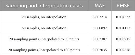
Table 4. MAE (m) and RMSE (m) of reconstructed curves.

The results indicate that both MAE, and RMSE, are lower for 50 sampling points without interpolation, or for 20 sampling points interpolated to 50 or 100 points, than for 20 sampling points without interpolation. This indicates that increasing the number of sampling points and applying interpolation can effectively reduce the reconstruction error. Furthermore, the relatively small MAE, and RMSE, values across all four cases demonstrate that the tangent angle recursive algorithm can accurately reconstruct the optical fiber curves, thereby confirming its feasibility and effectiveness.

4 Conclusion

In this paper, planar curve reconstruction for optical fiber sensors is addressed by integrating cubic spline interpolation with a tangent angle recursion algorithm. Discrete curvature is computed from fiber strain data based on an approximate relationship between wavelength and curvature. The curvature is then smoothed using cubic spline interpolation, and the curve is accurately reconstructed via the tangent angle recursion method. Results demonstrate that the reconstructed curves exhibit good smoothness and physical realism. The MAE and RMSE values obtained under different parameter settings validate the feasibility and reliability of the proposed method. This study offers both theoretical and experimental support for the advancement of optical fiber shape sensing technologies, highlighting their significant potential in high-precision applications such as medical instrumentation, aerospace structural monitoring, and infrastructure health assessment.

Data availability statement

The original contributions presented in the study are included in the article/supplementary material, further inquiries can be directed to the corresponding author.

Author contributions

YL: Investigation, Methodology, Software, Validation, Writing – original draft, Writing – review and editing. HJ: Funding acquisition, Investigation, Supervision, Writing – original draft, Writing – review and editing.

Funding

The author(s) declare that financial support was received for the research and/or publication of this article. This work was financially supported by the Xiangtan University College Student Innovation and Entrepreneurship Training Program, the National Natural Science Foundation of China (No. 51902276), the Natural Science Foundation of Hunan Province (No. 2019JJ50583, 2023JJ30585), the Scientific Research Fund of Hunan Provincial Education Department (No. 21B0111).

Conflict of interest

The authors declare that the research was conducted in the absence of any commercial or financial relationships that could be construed as a potential conflict of interest.

Generative AI statement

The author(s) declare that no Generative AI was used in the creation of this manuscript.

Any alternative text (alt text) provided alongside figures in this article has been generated by Frontiers with the support of artificial intelligence and reasonable efforts have been made to ensure accuracy, including review by the authors wherever possible. If you identify any issues, please contact us.

Publisher’s note

All claims expressed in this article are solely those of the authors and do not necessarily represent those of their affiliated organizations, or those of the publisher, the editors and the reviewers. Any product that may be evaluated in this article, or claim that may be made by its manufacturer, is not guaranteed or endorsed by the publisher.

References

1. Giallorenzi TG, Bucaro JA, Dandridge A, Sigel G, Cole J, Rashleigh S, et al. Optical fiber sensor technology. IEEE Trans microwave Theor Tech (1982) 30(4):472–511. doi:10.1109/tmtt.1982.1131089

CrossRef Full Text | Google Scholar

2. Lee B. Review of the present status of optical fiber sensors. Opt fiber Technol (2003) 9(2):57–79. doi:10.1016/s1068-5200(02)00527-8

CrossRef Full Text | Google Scholar

3. Hisham HK. Optical fiber sensing technology: basics, classifications and applications. Am J Remote Sens (2018) 6(1):1–5. doi:10.11648/j.ajrs.20180601.11

CrossRef Full Text | Google Scholar

4. Henken K, Van Gerwen D, Dankelman J, Van Den Dobbelsteen J. Accuracy of needle position measurements using fiber bragg gratings. Minimally Invasive Ther & Allied Tech (2012) 21(6):408–14. doi:10.3109/13645706.2012.666251

PubMed Abstract | CrossRef Full Text | Google Scholar

5. Khan F, Denasi A, Barrera D, Madrigal J, Sales S, Misra S. Multi-core optical fibers with bragg gratings as shape sensor for flexible medical instruments. IEEE sensors J (2019) 19(14):5878–84. doi:10.1109/jsen.2019.2905010

CrossRef Full Text | Google Scholar

6. Shuyang C, Fengze T, Weimin L, Luo H, Yu J, Qu J, et al. Deep learning-based ballistocardiography reconstruction algorithm on the optical fiber sensor. Opt express (2022) 30(8):13121–33. doi:10.1364/oe.452408

PubMed Abstract | CrossRef Full Text | Google Scholar

7. van de Berg NJ, Dankelman J, van den Dobbelsteen JJ. Design of an actively controlled steerable needle with tendon actuation and FBG-based shape sensing. Med Eng & Phys (2015) 37(6):617–22. doi:10.1016/j.medengphy.2015.03.016

PubMed Abstract | CrossRef Full Text | Google Scholar

8. Chen K, Fan H, Bao H. Discontinuous deformation monitoring of smart aerospace structures based on hybrid reconstruction strategy and fiber bragg grating. Sensors (2024) 24(11):3603. doi:10.3390/s24113603

PubMed Abstract | CrossRef Full Text | Google Scholar

9. Wang Y, Zhu L, He Y. Flexible skin-shaped optical fiber reconstruction method for allomorphic aircrafts. China Mech Eng (2023) 34(15):1873. doi:10.3969/j.issn.1004-132X.2023.15.012

CrossRef Full Text | Google Scholar

10. Ma Z, Chen X. Fiber bragg gratings sensors for aircraft wing shape measurement: recent applications and technical analysis. Sensors (2018) 19(1):55. doi:10.3390/s19010055

PubMed Abstract | CrossRef Full Text | Google Scholar

11. Detka M, Kaczmarek Z. Distributed strain reconstruction based on a fiber Bragg grating reflection spectrum. Metrology Meas Syst (2013) 20(1):53–64. doi:10.2478/mms-2013-0005

CrossRef Full Text | Google Scholar

12. Lei L, Qiwei X, Lai X. Morphological reconstruction of marine risers based on fiber optic sensing technology. J Optoelectronics- Laser (2024) 35(8):828–35. doi:10.16136/j.joel.2024.08.0864

CrossRef Full Text | Google Scholar

13. Jiabo L, Xu X, Cai C. Research on pipeline monitoring system based on fiber optic pressure sensor (in English). Infrared Laser Eng (2015) 44(11):3343–7. doi:10.3969/j.issn.1007-2276.2015.11.030

CrossRef Full Text | Google Scholar

14. Pauer H, Ledermann C, Woern H. Motivation of a new approach for shape reconstruction based on FBG-optical fibers: considering of the Bragg-gratings composition as a sensornetwork[C]. In: 2014 IEEE ninth international conference on intelligent sensors, sensor networks and information processing (ISSNIP). IEEE (2014). p. 1–5.

CrossRef Full Text | Google Scholar

15. Khan F, Donder A, Galvan S, Baena FR, Misra S. Pose measurement of flexible medical instruments using fiber Bragg gratings in multi-core fiber. IEEE Sensors J (2020) 20(18):10955–62. doi:10.1109/jsen.2020.2993452

CrossRef Full Text | Google Scholar

16. Jiahao L, Dong M, He Y. A multicore fiber reconstruction method for 3D shape of flexible mechanism introducing curvature and angle correction. Infrared Laser Eng (2021) 50(05):120–6. doi:10.3788/IRLA20200453

CrossRef Full Text | Google Scholar

17. Souza EA, Macedo LC, Frizera A, Marques C, Leal-Junior A. Fiber bragg grating array for shape reconstruction in structural elements. Sensors (2022) 22(17):6545. doi:10.3390/s22176545

PubMed Abstract | CrossRef Full Text | Google Scholar

18. Ferreira P, Caetano E, Ramos L, Pinto P. Shape sensing monitoring system based on fiber-optic strain measurements: laboratory tests. Exp Tech (2017) 41(4):407–20. doi:10.1007/s40799-017-0187-0

CrossRef Full Text | Google Scholar

19. Zhang Y, Xiao H, Shen L. Coordinate point fitting for fiber grating curve reconstruction algorithm. Opt Precision Dense Eng (2016) 24(09):2149–57. doi:10.3788/OPE.20162409.2149

CrossRef Full Text | Google Scholar

20. McKinley S, Levine M. Cubic spline interpolation. Coll Redwoods (1998) 45(1):1049–60.

Google Scholar

21. Dyer SA, Dyer JS. Cubic-spline interpolation. 1. IEEE Instrumentation & Meas Mag (2002) 4(1):44–6. doi:10.1109/5289.911175

CrossRef Full Text | Google Scholar

22. Kumar A, Govil LK. Interpolation of natural cubic spline. Int J Mathematics Math Sci (1992) 15(2):229–34. doi:10.1155/s0161171292000292

CrossRef Full Text | Google Scholar

23. Wu G, Qiao F, Fang X, Liang M, Song Y. Straightness perception mechanism of scraper conveyor based on the three-dimensional curvature sensing of FBG. Appl Sci (2023) 13(6):3619. doi:10.3390/app13063619

CrossRef Full Text | Google Scholar

24. Liu H, Bai Y. Wind turbine Tower state reconstruction method based on the corner cut recursion algorithm. Energies (2024) 17(8):1979. doi:10.3390/en17081979

CrossRef Full Text | Google Scholar

25. Lee HY, Liang CG. A new vector theory for the analysis of spatial mechanisms. Mechanism Machine Theor (1988) 23(3):209–17. doi:10.1016/0094-114x(88)90106-1

CrossRef Full Text | Google Scholar

26. Paloschi D, Bronnikov KA, Korganbayev S, Wolf AA, Dostovalov A, Saccomandi P. 3D shape sensing with multicore optical fibers: transformation matrices versus frenet-serret equations for real-time application. IEEE Sensors J (2020) 21(4):4599–609. doi:10.1109/jsen.2020.3032480

CrossRef Full Text | Google Scholar

27. Stewart J, Kokoska S. Calculus: concepts and contexts[M]. Toronto: Cengage Learning (2010).

Google Scholar

28. Chai T, Draxler RR. Root mean square error (RMSE) or mean absolute error (MAE). Geoscientific Model Development Discussions (2014) 7(1):1525–34. doi:10.5194/gmd-7-1247-2014

CrossRef Full Text | Google Scholar

29. Hodson TO. Root mean square error (RMSE) or mean absolute error (MAE): when to use them or not. Geoscientific Model Development Discuss (2022) 2022:5481–7. doi:10.5194/gmd-15-5481-2022

CrossRef Full Text | Google Scholar