Coherent manipulation of spatial bright solitons of reflection and transmission using control fields of Milnor Gaussian polynomials

The generation of spatial bright solitons of reflection and transmission pulses and their intensities are investigated in a sodium atomic medium using Gaussian Milnor polynomial control fields. Significant bright and dark ring-shaped solitons are controlled by balancing nonlinearity and dispersion along two spatial coordinates. The intensity is more localized along one of the spatial coordinates due to larger nonlinearity and spread along other spatial coordinates due to smaller nonlinearity in the reflection pulse. A circular, crater-type bright soliton intensity is also maintained around the origin of the x and y coordinates, exhibiting varying intensity along the circumference. A large, bright intensity peak is observed around the origin, with the intensity minima at the center in reflection. The intensity peaks are enhanced in one of the spatial coordinates and localized in another coordinate in reflection. A large Gaussian-type bright solitonic intensity distribution is investigated at approximately $y=0\lambda$ throughout the variation along the x-axis in the transmission pulse pattern. The reflection and transmission pulse intensities vary from $0\%$ to $40\%$ , and at least $20\%$ of the intensity of the incident pulse is lost by attenuation. The modified results are useful in optical communications, fiber optics, optical computation, signal processing, radar technology, and artificial neural networks.

1 Introduction

Solitons are spatial waves that stay together as they travel because the medium’s nonlinearity and spreading effects cancel each other out. The word “soliton” is used for a wave that looks like a single, short pulse that can pass through another similar pulse without changing its shape or speed [1]. They occur in various physical systems, such as fluids [2], optical fibers [3, 4], plasmas [5], condensed matter systems [6], acoustic media [7], and gravitational systems [8, 9]. Solitons have some key properties that distinguish them from other wave phenomena. Among these properties, shape preservation [10], stable propagation [11, 12], elastic collisions [13], stability [11], localized energy [15], nonlinear nature [16, 17], and robustness [18] are the most prominent. Solitons remain stable when the spreading effect (dispersion or diffraction) and the medium’s nonlinearity cancel each other out at a certain level of the applied control field [19]. Because of this balance, strong solitons can withstand disturbances such as fluctuations in light intensity or phase noise.

The history of solitons spans several centuries and involves contributions from multiple fields of science and mathematics. Early studies of waves in various media—such as the motion of water waves—laid the groundwork for understanding the wave behavior. However, the concept of a soliton had not yet formed in the early $19^{th}$ century [20]. John Scott Russell observed a phenomenon while traveling along a canal near Edinburgh, Scotland. He witnessed a single solitary wave traveling along the water that retained its shape and velocity over a long distance [21]. Solitons were theoretically developed in the 19th century, particularly with Korteweg–de Vries (KdV) equations [20] in 1895. The concept of solitons began to mature with the advent of nonlinear dynamics and solitary wave theory. In particular, the works of Mikhail M. Korteweg and Balthazar de Vries in the late 19th century contributed to the refinement of the soliton theory [23]. In 1970, the inverse scattering theory and solitons in mathematical physics gained great recognition [23]. In 1980, solitons played a vital role in nonlinear optics and fiber-optic communications [25]. In 2000, solitons were integrated into string theory and quantum field theory. Since then, solitons have been explored in numerous modern technologies, such as quantum computing, secure communication, and advanced optical systems [26–28].

Solitons have many types based on the physical systems in which they occur and the nature of the balance between nonlinearity and dispersion. The main types are bright solitons [29], dark solitons [30], vortex solitons [31], breathers [32], sine-Gordon solitons [33], and Korteweg–de Vries solitons [34], among others. Spatial bright solitons are self-trapped light beams that can travel through a nonlinear medium without spreading out. They form when the medium’s refractive index increases with light intensity, focusing the beam and balancing diffraction [35]. Solitons in the presence of Milnor polynomials involve studying soliton solutions within systems influenced by the structure of Milnor polynomials. Milnor polynomials arise in singularity theory and are used to describe the behavior of complex systems near critical points or singularities. When applied to nonlinear systems, these polynomials can introduce new potential landscapes that affect soliton dynamics. Solitons have applications in diverse fields of science and technology. The concept of solitons finds applications across a wide range of disciplines, such as optical communications [36–38], plasma physics [39], laser physics [40, 41], fluid dynamics [42, 43], magnetism, semiconductor and materials science [44, 45], chalcogenide glasses [46], nerve impulses [47, 48], fiber optics [49], optical computation [50], signal processing [51], radar technology [52], microcomb range measurement [53], and artificial neural networks [54].

In this work, we study the generation of spatial bright solitons of reflection and transmission pulses and their intensities in a sodium atomic medium using control fields of Gaussian Milnor polynomial. A significant gap in the study of optics will be filled by the updated result.

2 Model of the atomic system and its susceptibility

The sodium atomic system as shown in Figure 1, has a ground state $\left|1\right.⟩$ and additional states $\left|\mathrm{2,3,4}\right.⟩$ resulting from hyperfine splitting. In this atomic configuration, the probe field with Rabi frequency ${\mathrm{\Omega }}_p$ and detuning ${\mathrm{\Delta }}_p$ couples the lowest energy level $\left|1\right.⟩$ to the uppermost state $\left|4\right.⟩$ . The state $\left|2\right.⟩$ connects to levels $\left|3\right.⟩$ and $\left|4\right.⟩$ via control fields with Rabi frequencies ${\mathrm{\Omega }}_3$ and ${\mathrm{\Omega }}_1$ , respectively. Similarly, the state $\left|3\right.⟩$ interacts with the upper excited state $\left|4\right.⟩$ through a control field of Rabi frequency ${\mathrm{\Omega }}_2$ and detuning ${\mathrm{\Delta }}_2$ . The associated decay rates are given by ${\gamma }_{32}$ , ${\gamma }_{41}$ , ${\gamma }_{42}$ , and ${\gamma }_{43}$ .

Figure 1

Figure 1. Four-level sodium atomic medium.

The optical behavior of this atomic arrangement interacting with the probe and the three control fields is examined by analyzing its response. The Hamiltonian for the sodium atomic system is constructed in the interaction picture, employing the dipole approximation and the rotating wave approximation, in order to derive the required atomic susceptibility.

The Hamiltonian representing the configuration in the absence of external interactions is expressed as follows:

$H_0=\hslash {\omega }_2\left|2\right.⟩\left.⟨2\right|+\hslash {\omega }_1\left|1\right.⟩\left.⟨1\right|+\hslash {\omega }_4\left|4\right.⟩\left.⟨4\right|+\hslash {\omega }_3\left|3\right.⟩\left.⟨3\right|.(1)$

The Hamiltonian governing the system’s dynamics in the interaction picture is expressed as follows:

$\begin{array}{c}{H}_I=-\frac{\hslash }{2}[{\mathrm{\Omega }}_1{e}^{-i{\mathrm{\Delta }}_{1}t}\left|2\right.⟩\left.⟨4\right|+{\mathrm{\Omega }}_p{e}^{-i{\mathrm{\Delta }}_{p}t}\left|1\right.⟩\left.⟨4\right|+{\mathrm{\Omega }}_3{e}^{-i{\mathrm{\Delta }}_{3}t}\left|2\right.⟩\left.⟨3\right|\\ +{\mathrm{\Omega }}_2{e}^{-i{\mathrm{\Delta }}_{2}t}\left|3\right.⟩\left.⟨4\right|]+H.c.\end{array}(2)$

Equations 1, 2 represent the complete Hamiltonian of the system. The dynamics of the atomic system in the Heisenberg picture are governed by the density matrix formalism, which is calculated as follows:

$\frac{d}{dt}\rho =-\frac{i}{\hslash }\left[H_I,\rho \right]-\frac{1}{2}\sum {\gamma }_{ij}\left(-2\sigma \rho {\sigma }^{†}+{\sigma }^{†}\sigma \rho +\rho {\sigma }^{†}\sigma \right).(3)$

In Equation 3, $\rho$ indicates the operator elements of the density matrix, whereas ${\sigma }^{†}$ and $\sigma$ denote the creation (raising) and annihilation (lowering) operators, respectively. The decay processes between the energy levels are described by the coefficients ${\gamma }_{ij}$ for $i,j=\mathrm{1,2,3,4}$ . The system yields a set of coupling equations that do not explicitly depend on time. At the initial moment, the atoms are assumed to be entirely in the ground state $\left|1\right.⟩$ , which sets the initial density element to ${\tilde{\rho }}_{11}^{(0)}=\left|1\right.⟩$ . Consequently, the excited states are unoccupied at the start, implying that ${\tilde{\rho }}_{44}^{(0)}={\tilde{\rho }}_{43}^{(0)}={\tilde{\rho }}_{42}^{(0)}=0$ . Using a first-order perturbative expansion, the density matrix equations can be simplified and solved through the use of the following relation:

$P=M^{-1}Q.(4)$

In Equation 4, $X(t)$ and $M$ are treated as column vectors, whereas $Y$ represents a $3\times 3$ matrix. The resulting expression for the probe coherence element, ${\tilde{\rho }}_{14}$ , is given as follows:

${\tilde{\rho }}_{14}=\frac{-\left(a_2{a}_3+{\mathrm{\Omega }}_2^2\right){\mathrm{\Omega }}_p}{F-2i\left(4a_1{a}_2{a}_3+a_3{\mathrm{\Omega }}_1^2+a_1{\mathrm{\Omega }}_2^2+a_2{\mathrm{\Omega }}_3^2\right)}.(5)$

To introduce cross Kerr nonlinearity in ${\tilde{\rho }}_{14}$ as shown in Equation 5, we expanded ${\tilde{\rho }}_{14}$ in the manner ${\tilde{\rho }}_{14}(k)={\tilde{\rho }}_{14}(0)+I\frac{\partial {\rho }_{14}}{\partial {\mathrm{\Omega }}_1}{|}_{{\mathrm{\Omega }}_1->0}$ , where ${\tilde{\rho }}_{14}(0)$ is probe coherence without the Kerr-nonlinearity and ${\partial }_{{\mathrm{\Omega }}_1}^2{\tilde{\rho }}_{14}{|}_{{\mathrm{\Omega }}_1->0}$ shows the cross Kerr effect coherence and $I={\mathrm{\Omega }}_1^2$ Kerr field intensity. The dispersion is related to the derivative of susceptibility with the respected probe detuning, such as $Dispersion=\frac{\partial \mathrm{R}\mathrm{e}[\chi ]}{\partial {\mathrm{\Delta }}_p}$ ,

where

$\begin{array}{ccc}\hfill & \hfill & a_1=-\frac{1}{2}\left({\gamma }_{41}+{\gamma }_{21}\right)+i{\mathrm{\Delta }}_p,a_2=i\left(-{\mathrm{\Delta }}_1+{\mathrm{\Delta }}_p\right)-\frac{1}{2}{\gamma }_{32},a_3=i\left(-{\mathrm{\Delta }}_3+{\mathrm{\Delta }}_p\right)-\frac{1}{2}{\gamma }_{43},\hfill \\ \hfill & \hfill & F={\mathrm{\Omega }}_1{\mathrm{\Omega }}_2{\mathrm{\Omega }}_3\left[\exp \left(i\phi \right)+\exp \left(-i\phi \right)\right].\hfill \end{array}$

The Rabi frequencies of the control light fields in the form of Gaussian Minor polynomial are written as follows:

${\mathrm{\Omega }}_1=G_1\exp \left[\frac{-r^2}{2W}\right]\left(1-r^2-r^4+r^6-8r^3{e}^{3i{\varphi }_1}\right),(6)$

${\mathrm{\Omega }}_2=G_2\exp \left[\frac{-r^2}{2W}\right]\left(1-r^2-r^4+r^6-8r^3{e}^{3i{\varphi }_2}\right),(7)$

${\mathrm{\Omega }}_3=G_3\exp \left[\frac{-r^2}{2W}\right]\left(1-r^2-r^4+r^6-8r^3{e}^{3i{\varphi }_3}\right),(8)$

In Equations 6–8, $W$ is the beam waist, $G_{\mathrm{1,2,3}}$ are the associated field strengths, and $r=\sqrt{x^2+y^2}$ . For this four-level sodium atom scheme, the resulting complex susceptibility takes the form. Gaussian Minor polynomial generated optical knot behaviors in pulses and was more informative than standard Gaussian or Laguerre-Gaussian profiles,

$\chi =\frac{2N{\wp }_{14}^2}{{\epsilon }_0\hslash {\mathrm{\Omega }}_p}{\tilde{\rho }}_{14}\left(k\right),(9)$

where, in Equation 9, $N$ represents the atomic density. ${\epsilon }_0$ corresponds to the permittivity of free space and $\hslash$ is the reduced plank constant and

${\wp }_{14}=\sqrt{\frac{3\hslash {\gamma }_{41}{\epsilon }_0{\lambda }^3}{8{\pi }^2}}.(10)$

Equation 10 represent the dipole matrix element. The group index characterizing the medium can be expressed as follows:

$n_g=2\pi \omega \mathrm{R}\mathrm{e}\left({\partial }_{\mathrm{\Delta }p}\chi \right)+2\pi \mathrm{R}\mathrm{e}\left(\chi \right)+1,(11)$

where, in Equation 11, $n_g$ is the group index. The group velocity $v_g$ can be written as follows:

$v_g=\frac{c}{2\pi \omega \mathrm{R}\mathrm{e}\left({\partial }_{\mathrm{\Delta }p}\chi \right)+2\pi \mathrm{R}\mathrm{e}\left(\chi \right)+1}.(12)$

The group index expression in Equation 12, show the fast or slow propagation of solitons waves. The reflection and transmission are written as follows:

$R\left({\mathrm{\Delta }}_i,x,y,G_i,{\gamma }_{ij}\right)=\frac{u_3\sin \left({\alpha }_2\right)+\left({\xi }_0^2-{\xi }_1^2\right){\xi }_1{\xi }_2\sin 2{\alpha }_1\cos \left({\alpha }_2\right)}{u_2\sin \left({\alpha }_2\right)+{\xi }_1{\xi }_2{u}_1\cos \left({\alpha }_2\right)},(13)$

$T\left({\mathrm{\Delta }}_i,x,y,G_i,{\gamma }_{ij}\right)=\frac{2i{\xi }_0{\xi }_2{\xi }_1^2}{u_2\sin \left({\alpha }_2\right)+{\xi }_1{\xi }_2{u}_1\cos \left({\alpha }_2\right)},(14)$

where, in Equations 13, 14 the terms $u_{1,2,3}$ are given as

$\begin{array}{c}{u}_1=2i{\xi }_0{\xi }_1\cos 2{\alpha }_1+\left({\xi }_0^2+{\xi }_1^2\right)\sin 2{\alpha }_1,\hfill \\ u_2={\xi }_1^2\left({\xi }_0^2+{\xi }_2^2\right){\cos }^2{\alpha }_1-\left({\xi }_1^4+{\xi }_0^2{\xi }_2^2\right){\sin }^2{\alpha }_1-i{\xi }_0{\xi }_1\left({\xi }_1^2+{\xi }_2^2\right)\sin 2{\alpha }_1,\hfill \\ u_3={\xi }_1^2\left({\xi }_0^2-{\xi }_2^2\right){\cos }^2{\alpha }_1+\left({\xi }_1^4-{\xi }_0^2{\xi }_2^2\right){\sin }^2{\alpha }_1.\hfill \end{array}$

At the plane $z=0$ , the incident probe beam is represented as follows:

$E_i\left(x,y\right){|}_{z=0}=\frac{1}{2\pi }{\int }_{-\infty }^{\infty }{e}^{i\left(k_{z}z+k_{y}y\right)}A\left({\omega }_p,k_y\right)d{k}_y,(15)$

where, in Equation 15 the term “A” is described as

$A\left({\omega }_p,k_y\right)=\frac{W_y}{\sqrt{2}}{e}^{-\frac{W_y^2{\left(k_y-k_{y0}\right)}^2}{4}}.$

The mathematical expressions for the transmitted and reflected pulses are given below.

$E_t\left(x,y\right)=\frac{1}{2\pi }{\int }_{-\infty }^{\infty }T\left(x,y,{\mathrm{\Delta }}_i,G_i,{\gamma }_{ij}\right)A\left({\omega }_p,k_y\right)e^{i\left(k_z\left(z-L\right)+k_{y}y\right)}d{k}_y,(16)$

$E_r\left(x,y\right)=\frac{1}{2\pi }{\int }_{-\infty }^{\infty }R\left(x,y,{\mathrm{\Delta }}_i,G_i,{\gamma }_{ij}\right)A\left(k_y,{\omega }_p\right)e^{i\left(-k_{z}z+k_{y}y\right)}d{k}_y,(17)$

In Equations 16, 17, $E_r(x,y)$ represents the pulse variation of the reflection beam and $E_t(x,y)$ represents the pulse variation of the transmission beam. These pulses are taken in full domain, and their boundaries are from $-\infty$ to $+\infty$ . The intensities of the reflection and transmission beams are $I_r{(x,y)}_R=|E_r(x,y){|}^2$ and $I_t(x,y)=|E_t(x,y){|}^2$ , respectively.

3 Results and discussion

The results are presented to demonstrate the generation of spatial bright solitons for both the reflected and transmitted pulses, as well as their corresponding intensities. This is achieved by applying control fields that have a shape described by a Gaussian Milnor polynomial within a sodium atomic medium. A decay rate of $\mathrm{\Gamma }=1GHz$ is used as the reference value, and all other frequency-related parameters are expressed in units scaled by this decay rate $\gamma$ . Throughout this work, atomic units are consistently employed for all calculations. Furthermore, $\omega =\mathrm{1,000}\gamma$ , $d=2d_1+d_2$ , $\lambda =2\pi c/\omega$ , $r=\sqrt{x^2+y^2}$ . ${\epsilon }_1=2.2$ , ${\epsilon }_2=1+4\pi \mathrm{R}\mathrm{e}(\chi )$ , $d_1=1.5\lambda$ , $d_2=15\lambda$ , $k_0=\omega /c$ , and $z=0.1\lambda$ . $w=2.5\lambda$ , where $k_z=\frac{2\pi }{\lambda }\cos \theta$ ; $w_y=w\sec \theta$ , where ${\epsilon }_2=1+\chi$ , ${\xi }_{\mathrm{0,1}}=\sqrt{{\epsilon }_{\mathrm{0,1}}-{\sin }^2\theta }$ , ${\xi }_2=\sqrt{{\epsilon }_2-{\sin }^2\theta }$ , ${\alpha }_1=\frac{2\pi }{\lambda }{d}_1\sqrt{{\epsilon }_1-{\sin }^2\theta }$ , and ${\alpha }_2=\frac{2\pi }{\lambda }{d}_2{\xi }_2$ . The nonlinearity is generated by the expansion of susceptibility with respect to Rabi frequency ${\mathrm{\Omega }}_1$ , and higher-order Kerr effect is ignored in the system.

In Figure 2, the charts depict the reflection pulse and reflection pulse intensity against wavelength-normalized $y$ and $x$ positions through a four-level sodium atomic medium. Periodic bright and dark soliton behaviors are obtained with variations of $y/\lambda$ and $x/\lambda$ . Sketches are presented for the reflection pulse and intensity at the chosen parameters of ${\mathrm{\Delta }}_1=0.2\mathrm{\Gamma }$ , ${\mathrm{\Delta }}_3=0.2\mathrm{\Gamma }$ , ${\mathrm{\Delta }}_p=0\mathrm{\Gamma }$ , $\phi =\pi /2$ , $G_{\mathrm{1,2,3}}=5\mathrm{\Gamma }$ , $\theta =\pi /3$ , ${\varphi }_1=\pi /6$ , ${\varphi }_3=\pi /3$ , ${\tau }_0=1/\mathrm{\Gamma }$ , and ${\varphi }_2=\pi /4$ . The reflection pulse $E_r(x,y)$ shows periodic bright and dark soliton behaviors with large nonlinearity and minimum dispersion along the y-axis and small nonlinearity and larger dispersion along the x-axis. The bright soliton is formed by balancing Kerr nonlinearity and anomalous dispersion, whereas the dark soliton is formed by balancing Kerr nonlinearity and normal dispersion in this work. The pulse is more localized along the y-axis due to large nonlinearity and spread along the x-axis due to small nonlinearity. Stability is obtained through balancing nonlinearity and dispersion, and a stable periodic soliton is controlled. The pulse behaviors are periodic mostly along the y-axis and solitonic vectors along the x-axis. Three bright ring-type solitonic shapes are also controlled, as shown in Figure 2a, and their clear density plots are shown in Figure 2c. The intensity of reflection pulse $I_r(x,y)=|E_r(x,y){|}^2$ is also a varying function of wavelength-normalized $y$ and $x$ positions. The reflection pulse intensity varies from $0\%$ to $40\%$ .The intensity is more localized along one of the spatial coordinates, the y-axis, due to larger nonlinearity and spread along the other spatial coordinate, the x-axis, due to smaller nonlinearity. A circular ring-type right soliton intensity is also controlled around the origin of the x and y coordinates, as shown in Figure 2b. This is clearer in their density plots, as shown in Figure 2d.

Figure 2

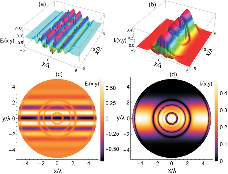
Figure 2. Reflection pulse and reflection pulse intensity versus the spatial axes $x/\lambda$ and $y/\lambda$ . The proposed parameters are ${\gamma }_{\mathrm{32,41,42,43}}=2\mathrm{\Gamma }$ , ${\mathrm{\Delta }}_1=0.2\mathrm{\Gamma }$ , ${\mathrm{\Delta }}_3=0.2\mathrm{\Gamma }$ , ${\mathrm{\Delta }}_p=0\mathrm{\Gamma }$ , $\phi =\pi /2$ , $G_{\mathrm{1,2,3}}=5\mathrm{\Gamma }$ , $\theta =\pi /3$ , ${\varphi }_2=\pi /4$ , ${\tau }_0=1/\mathrm{\Gamma }$ , ${\varphi }_1=\pi /6$ , and ${\varphi }_3=\pi /3$ . Panel (a) is the soliton pulse, panel (b) is its intensity, panel (c) is the density plot of (a), and panel (d) is the density plot of (b).

The graphs in Figure 3 visualize the transmission pulse and transmission pulse intensity against wavelength-normalized $x$ and $y$ positions through a four-level sodium atomic medium. The plots for transmission pulse and their intensity are traced at the parameters shown in Figure 3. Vector bright and dark soliton behaviors are obtained with variations of $y/\lambda$ and $x/\lambda$ in the transmission pulse. The transmission pulse $E_t(x,y)$ shows periodic bright and dark soliton behavior along both wavelength-normalized $x$ and $y$ positions. The nonlinearity is larger along the y-axis and small along the x-axis at the mentioned parameters. Stability is obtained through balancing nonlinearity and dispersion. The pulse behaviors are periodic mostly along the x and y axes and solitonic vectors along the x and y axes. Ring-type bright and dark solitonic shapes are also controlled, as shown in Figure 3a. The transmission pulse density plot is visualized in Figure 3c. The intensity of transmission pulse $I_t(x,y)=|E_t(x,y){|}^2$ is also a varying function of the spatial coordinates $x/\lambda$ and $y/\lambda$ . The transmission pulse intensity also varies from $0\%$ to $40\%$ .The intensity is more localized along one of the spatial coordinates, the y-axis, due to larger nonlinearity and spread along the other spatial coordinate, the x-axis, due to smaller nonlinearity. A circular crater-type bright soliton intensity is also controlled around the origin of the $x$ and $y$ axes, having varying intensity at the circumference length, as shown in Figure 3b. This is clearer in their density plots shown in Figure 3d.

Figure 3

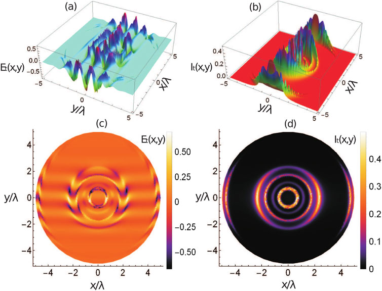
Figure 3. Transmission pulse and transmission pulse intensity versus wavelength-normalized $x$ and $y$ positions. The proposed parameters are ${\gamma }_{\mathrm{32,41,42,43}}=2\mathrm{\Gamma }$ , ${\mathrm{\Delta }}_1=0.2\mathrm{\Gamma }$ , ${\mathrm{\Delta }}_3=0.2\mathrm{\Gamma }$ , ${\mathrm{\Delta }}_p=0\mathrm{\Gamma }$ , $\phi =\pi /2$ , $G_{\mathrm{1,2,3}}=5\mathrm{\Gamma }$ , $\theta =\pi /3$ , ${\varphi }_1=\pi /6$ , ${\varphi }_2=\pi /4$ , ${\varphi }_3=\pi /3$ , and ${\tau }_0=1/\mathrm{\Gamma }$ . Panel (a) is the soliton pulse, panel (b) is its intensity, panel (c) is the density plot of (a), and panel (d) is the density plot of (b).

In Figure 4, illustrations are presented for the reflection pulse and reflection pulse intensity against wavelength-normalized $x$ and $y$ positions through a four-level sodium atomic medium. The periodic vectors’ bright and dark soliton behaviors are investigated with the variation of wavelength-normalized $x$ and $y$ positions. At the parameters of ${\mathrm{\Delta }}_1=0.2\mathrm{\Gamma }$ , ${\mathrm{\Delta }}_3=0.2\mathrm{\Gamma }$ , ${\mathrm{\Delta }}_p=0\mathrm{\Gamma }$ , $\phi =\pi /2$ , $G_{\mathrm{1,2,3}}=5\mathrm{\Gamma }$ , $\theta =\pi /4$ , ${\varphi }_{\mathrm{1,2,3}}=0$ , and ${\tau }_0=1/\mathrm{\Gamma }$ , nonlinearity is smaller along the x-axis, and the pulse is spread, whereas nonlinearity is again larger along the y-axis, and the pulse is more localized in the reflection pulse pattern. The reflection pulse $E_r(x,y)$ shows periodic bright and dark soliton behavior with large nonlinearity and minimum dispersion along the y-axis and small nonlinearity and larger dispersion along the x-axis. The pulse is more localized along the y-axis due to large nonlinearity and spread along the x-axis due to small nonlinearity. The pulse behavior is mostly localized along the y-axis and solitonic along the x-axis of the spatial coordinates. A bright ring soliton at the origin and a larger circular bright ring soliton around the origin are investigated. Furthermore, at $y=0\lambda$ along the x-axis, a periodic dark soliton is investigated, whereas around the x-axis, $y\ne 0$ on both sides, bright solitons are controlled, as presented in Figure 4a, and their clear density plots are shown in Figure 4c. The intensity of the reflection pulse $I_r(x,y)=|E_r(x,y){|}^2$ is also a strong varying function of wavelength-normalized axes $x/\lambda$ and $y/\lambda$ . The reflection pulse intensity varies from $0\%$ to $1.5\%$ . A large bright intensity peak around the origin is investigated, which has intensity minima at the center at the origin. The intensity is more localized along one of the spatial coordinates, the y-axis, due to larger nonlinearity and spread along the other spatial coordinate, the x-axis, due to smaller nonlinearity. The intensity peaks are enhanced in one of the spatial coordinates (x-axis) and localized in the other coordinate (y-axis) in reflection, as shown in Figure 4b. This is clearer in their density plots, as shown in Figure 4d.

Figure 4

Figure 4. Reflection pulse and reflection pulse intensity versus wavelength-normalized $x$ and $y$ positions. The proposed parameters are ${\gamma }_{\mathrm{32,41,42,43}}=2\mathrm{\Gamma }$ , ${\mathrm{\Delta }}_1=0.2\mathrm{\Gamma }$ , ${\mathrm{\Delta }}_3=0.2\mathrm{\Gamma }$ , ${\mathrm{\Delta }}_p=0\mathrm{\Gamma }$ , $\phi =\pi /2$ , $G_{\mathrm{1,2,3}}=5\mathrm{\Gamma }$ , $\theta =\pi /4$ , ${\varphi }_{\mathrm{1,2,3}}=0$ , and ${\tau }_0=1/\mathrm{\Gamma }$ . Panel (a) is the soliton pulse, panel (b) is its intensity, panel (c) is the density plot of (a), and panel (d) is the density plot of (b).

Figure 5 presents the illustrations for the transmission pulse and transmission pulse intensity versus the spatial coordinates $y/\lambda$ and $x/\lambda$ . At the parameters of ${\mathrm{\Delta }}_1=0.2\mathrm{\Gamma }$ , ${\mathrm{\Delta }}_3=0.2\mathrm{\Gamma }$ , ${\mathrm{\Delta }}_p=0\mathrm{\Gamma }$ , $\phi =\pi /2$ , $G_{\mathrm{1,2,3}}=5\mathrm{\Gamma }$ , $\theta =\pi /4$ , ${\varphi }_{\mathrm{1,2,3}}=0$ , and ${\tau }_0=1/\mathrm{\Gamma }$ , nonlinearity is smaller along the x-axis and the pulse is spread, whereas along the y-axis, nonlinearity is larger and the pulse is more localized in the transmission pulse spectrum. The transmission pulse $E_t(x,y)$ is a vector of bright and dark soliton behaviors at $y=0\lambda$ along the x-axis. At approximately $y=0\lambda$ along the x-axis on both sides, dark soliton behaviors exist in the transmission pulse pattern, as presented in Figure 5a, and their clear density plots are shown in Figure 5c. The intensity of the transmission pulse $I_t(x,y)=|E_r(x,y){|}^2$ is uniform along the x-axis and more localized along the y-axis and is a function of $x/\lambda$ and $y/\lambda$ . The transmission pulse intensity varies from $0\%$ to $50\%$ . A large Gaussian bright intensity distribution is investigated at approximately $y=0\lambda$ throughout the variation along the x-axis. The intensity is more localized along one of the spatial coordinates, the y-axis, due to larger nonlinearity and spread along the other spatial coordinate, the x-axis, due to smaller nonlinearity. Furthermore, the intensity peak is Gaussian and has the minimum uncertainty, as shown in Figure 5b. This is clearer in the density plot of the transmission spectrum in Figure 5d.

Figure 5

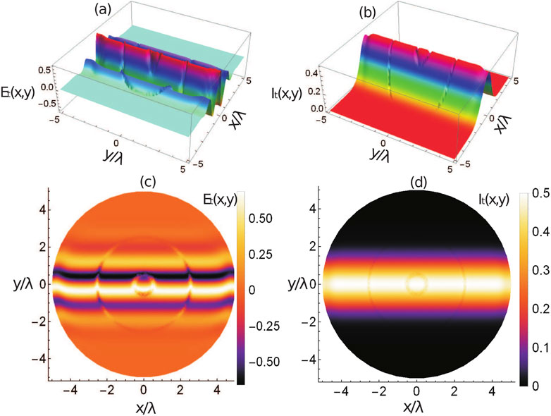
Figure 5. Transmission pulse and transmission pulse intensity versus wavelength-normalized $x$ and $y$ positions. The proposed parameters are ${\gamma }_{\mathrm{32,41,42,43}}=2\mathrm{\Gamma }$ , ${\mathrm{\Delta }}_1=0.2\mathrm{\Gamma }$ , ${\mathrm{\Delta }}_3=0.2\mathrm{\Gamma }$ , ${\mathrm{\Delta }}_p=0\mathrm{\Gamma }$ , $\phi =\pi /2$ , $G_{\mathrm{1,2,3}}=5\mathrm{\Gamma }$ , $\theta =\pi /4$ , ${\varphi }_{\mathrm{1,2,3}}=0$ , and ${\tau }_0=1/\mathrm{\Gamma }$ . Panel (a) is the soliton pulse, panel (b) is its intensity, panel (c) is the density plot of (a), and panel (d) is the density plot of (b).

4 Conclusion

The formation of spatial bright solitons in the reflected and transmitted pulses, along with their intensities, is examined in a sodium atomic medium by applying control fields shaped as Gaussian Milnor polynomials. A four-level sodium atomic system is driven by a weak probe field and three control fields, with the control fields having the Gaussian Milnor polynomial profile, to control and tune the bright and dark solitons in the reflected and transmitted beams. The density matrix formalism is utilized to calculate the electric susceptibility of the medium, and the dielectric function is derived from it. The reflection and transmission coefficients are determined using this dielectric function. These coefficients are then used to obtain the reflected and transmitted pulses and their respective intensities. Finally, the behavior of the reflected and transmitted pulses and their intensities is analyzed by plotting them against spatial coordinates normalized to the free-space wavelength of light. Significant bright and dark ring-shaped solitons are controlled by balancing nonlinearity and anomalous/normal dispersion along the two spatial coordinates. The intensity is more localized along one of the spatial coordinates due to larger nonlinearity and spread along other spatial coordinate due to smaller nonlinearity in the reflection pulse. A circular crater-type bright soliton intensity is also controlled around the origin of the x and y coordinates, having varying intensity at the circumference length. A large bright intensity peak around the origin is investigated, which has intensity minima at the center in the reflection. The intensity peaks are enhanced in one of the spatial coordinates and localized in the other coordinate in reflection. A large Gaussian-type bright solitonic intensity distribution is investigated at approximately $y=0\lambda$ throughout the variation along the x-axis in the transmission pulse pattern. The reflection and transmission pulse intensities both vary from $0\%$ to $40\%$ , and at least $20\%$ of the intensity of the incident pulse is lost. The maximum of the reflection pulse intensity is $40\%$ , and the maximum of the transmission pulse intensity is $40\%$ . The total sum of the reflection and transmission pulses are $80\%$ , and the remaining $20\%$ energy of the pulse is lost in the medium to other forms of energy, such as heat and internal molecular configuration.

Data availability statement

The raw data supporting the conclusions of this article will be made available by the authors, without undue reservation.

Author contributions

FA: Conceptualization, Investigation, Methodology, Validation, Visualization, Writing – original draft. DP: Conceptualization, Data curation, Funding acquisition, Investigation, Project administration, Supervision, Validation, Writing – review and editing. MD: Conceptualization, Formal Analysis, Methodology, Software, Validation, Writing – original draft. AM: Conceptualization, Data curation, Formal Analysis, Investigation, Methodology, Validation, Visualization, Writing – original draft. AA: Conceptualization, Formal Analysis, Investigation, Software, Supervision, Writing – review and editing.

Funding

The author(s) declare that financial support was received for the research and/or publication of this article.

Acknowledgments

The authors extend their appreciation to the Deanship of Research and Graduate Studies at King Khalid University for funding this work through Large Research Project under grant number “RGP. 2/145/46”, the authors also express their appreciation to the Deanship of Scientific Research at Northern Border University, Arar, Saudi Arabia for funding this research work through project number “NBU-FFR-2025-1324-04”.

Conflict of interest

The authors declare that the research was conducted in the absence of any commercial or financial relationships that could be construed as a potential conflict of interest.

Generative AI statement

The author(s) declare that no Generative AI was used in the creation of this manuscript.

Any alternative text (alt text) provided alongside figures in this article has been generated by Frontiers with the support of artificial intelligence and reasonable efforts have been made to ensure accuracy, including review by the authors wherever possible. If you identify any issues, please contact us.

Publisher’s note

All claims expressed in this article are solely those of the authors and do not necessarily represent those of their affiliated organizations, or those of the publisher, the editors and the reviewers. Any product that may be evaluated in this article, or claim that may be made by its manufacturer, is not guaranteed or endorsed by the publisher.

References

1. Scott AC, Chu FY, McLaughlin DW. The soliton: a new concept in applied science. Proc IEEE (1973) 61(10):1443–83. doi:10.1109/proc.1973.9296

CrossRef Full Text | Google Scholar

2. Gottwald G, Grimshaw R, Malomed BA. Stable two-dimensional parametric solitons in fluid systems. Phys Lett A (1998) 248(2-4):208–18. doi:10.1016/s0375-9601(98)00658-6

CrossRef Full Text | Google Scholar

3. Mollenauer LF, Gordon JP. Solitons in optical fibers: fundamentals and applications. Elsevier (2006).

Google Scholar

4. Hasegawa A, Kodama Y. Guiding-center soliton in optical fibers. Opt Lett (1990) 15(24):1443–5. doi:10.1364/ol.15.001443

PubMed Abstract | CrossRef Full Text | Google Scholar

5. Ichikawa YH. Topics on solitons in plasmas. Physica Scripta (1979) 20(3-4):296–305. doi:10.1088/0031-8949/20/3-4/002

CrossRef Full Text | Google Scholar

6. Bishop AR, Krumhansl JA, Trullinger SE. Solitons in condensed matter: a paradigm. Physica D: Nonlinear Phenomena (1980) 1(1):1–44. doi:10.1016/0167-2789(80)90003-2

CrossRef Full Text | Google Scholar

7. Ewen JF, Gunshor RL, Weston VH. An analysis of solitons in surface acoustic wave devices. J Appl Phys (1982) 53(8):5682–8. doi:10.1063/1.331454

CrossRef Full Text | Google Scholar

8. Belinski V, Verdaguer E, Gravitational solitons, (2001).

Google Scholar

9. Villatoro FR. Nonlinear gravitational waves and solitons. Nonlinear systems. Math Theor Comput Methods (2018) 1:207–40. doi:10.1007/978-3-319-66766-9_7

CrossRef Full Text | Google Scholar

10. Wang L, Gao YT, Meng DX, Gai XL, Xu PB. Soliton-shape-preserving and soliton-complex interactions for a (1+ 1)-dimensional nonlinear dispersive-wave system in shallow water. Nonlinear Dyn (2011) 66:161–8. doi:10.1007/s11071-010-9918-9

CrossRef Full Text | Google Scholar

11. Tao T. Why are solitons stable? Bull Am Math Soc (2009) 46(1):1–33. doi:10.1090/s0273-0979-08-01228-7

CrossRef Full Text | Google Scholar

12. Enns RH, Rangnekar SS, Kaplan AE. Bistable-soliton pulse propagation: stability aspects. Phys Rev A (1987) 36(3):1270–9. doi:10.1103/physreva.36.1270

PubMed Abstract | CrossRef Full Text | Google Scholar

13. Darvishi MT, Kavitha L, Najafi M, Kumar VS. Elastic collision of Mobile solitons of a (3+ 1)-dimensional soliton equation. Nonlinear Dyn (2016) 86:765–78. doi:10.1007/s11071-016-2920-0

CrossRef Full Text | Google Scholar

15. Timm L, Weimer H, Santos L, Mehlstaubler TE. Energy localization in an atomic chain with a topological soliton. Phys Rev Res (2020) 2(3):033198. doi:10.1103/physrevresearch.2.033198

CrossRef Full Text | Google Scholar

16. Kartashov YV, Malomed BA, Torner L. Solitons in nonlinear lattices. Rev Mod Phys (2011) 83(1):247–305. doi:10.1103/revmodphys.83.247

CrossRef Full Text | Google Scholar

17. Ali A, Ahmad J, Javed S. Exploring the dynamic nature of soliton solutions to the fractional coupled nonlinear schrodinger model with their sensitivity analysis. Opt Quan Electronics (2023) 55(9):810. doi:10.1007/s11082-023-05033-y

CrossRef Full Text | Google Scholar

18. Menyuk CR. Soliton robustness in optical fibers. JOSA B (1993) 10(9):1585–91. doi:10.1364/josab.10.001585

CrossRef Full Text | Google Scholar

19. Ullah I, Majeed A, Ali A, Khan ZA. Reflection and transmission solitons via high magneto optical medium. Chaos, Solitons and Fractals (2025) 191:115881. doi:10.1016/j.chaos.2024.115881

CrossRef Full Text | Google Scholar

20. Korteweg DJ, De Vries G. XLI. On the change of form of long waves advancing in a rectangular canal, and on a new type of long stationary waves. The Lond Edinb Dublin Philosophical Mag J Sci (1895) 39(240):422–43. doi:10.1080/14786449508620739

CrossRef Full Text | Google Scholar

21. Russell JS, Report on waves: made to the meetings of the British association in 1842-43, (1845).

Google Scholar

23. Zabusky NJ, Kruskal MD. Interaction of “solitons” in a collisionless plasma and the recurrence of initial states. Phys Rev Lett (1965) 15(6):240–3. doi:10.1103/physrevlett.15.240

CrossRef Full Text | Google Scholar

25. Piekara A. 6A7-On self-trapping of a laser beam. IEEE J Quan Electronics (1966) 2(8):249–50. doi:10.1109/jqe.1966.1074035

CrossRef Full Text | Google Scholar

26. Zhou G, Xu J, Hu H, Liu Z, Zhang H, Xu C, et al. Off-axis four-reflection optical structure for lightweight single-band bathymetric LiDAR. IEEE Trans Geosci Remote Sensing (2023) 61:1–17. doi:10.1109/tgrs.2023.3298531

CrossRef Full Text | Google Scholar

27. Luo K, Fu Q, Liu X, Zhao R, He Q, Hu B, et al. Study of polarization transmission characteristics in nonspherical media. Opt Lasers Eng (2024) 174:107970. doi:10.1016/j.optlaseng.2023.107970

CrossRef Full Text | Google Scholar

28. Dong C, Fu Q, Wang K, Zong F, Li M, He Q, et al. The model and characteristics of polarized light transmission applicable to polydispersity particle underwater environment. Opt Lasers Eng (2024) 182:108449. doi:10.1016/j.optlaseng.2024.108449

CrossRef Full Text | Google Scholar

29. Khaykovich L, Schreck F, Ferrari G, Bourdel T, Cubizolles J, Carr LD, et al. Formation of a matter-wave bright soliton. Science (2002) 296(5571):1290–3. doi:10.1126/science.1071021

PubMed Abstract | CrossRef Full Text | Google Scholar

30. Kivshar YS, Luther-Davies B. Dark optical solitons: physics and applications. Phys Rep (1998) 298(2-3):81–197. doi:10.1016/s0370-1573(97)00073-2

CrossRef Full Text | Google Scholar

31. Malomed BA. Vortex solitons: old results and new perspectives. Physica D: Nonlinear Phenomena (2019) 399:108–37. doi:10.1016/j.physd.2019.04.009

CrossRef Full Text | Google Scholar

32. Yu M, Jang JK, Okawachi Y, Griffith AG, Luke K, Miller SA, et al. Breather soliton dynamics in microresonators. Nat Commun (2017) 8(1):14569. doi:10.1038/ncomms14569

PubMed Abstract | CrossRef Full Text | Google Scholar

33. Davidson A, Dueholm B, Kryger B, Pedersen NF. Experimental investigation of trapped sine-Gordon solitons. Phys Rev Lett (1985) 55(19):2059–62. doi:10.1103/physrevlett.55.2059

PubMed Abstract | CrossRef Full Text | Google Scholar

34. Pomeau Y, Ramani A, Grammaticos B. Structural stability of the Korteweg-de vries solitons under a singular perturbation. Physica D: Nonlinear Phenomena (1988) 31(1):127–34. doi:10.1016/0167-2789(88)90018-8

CrossRef Full Text | Google Scholar

35. Stegeman GI, Segev M. Bright spatial soliton interactions. In: Optical solitons: theoretical challenges and industrial perspectives: Les Houches Workshop (1999). 313–34. Berlin, Heidelberg: Springer Berlin Heidelberg.

Google Scholar

36. Haus HA, Wong WS. Solitons in optical communications. Rev Mod Phys (1996) 68(2):423–44. doi:10.1103/revmodphys.68.423

CrossRef Full Text | Google Scholar

37. Doran N, Blow K. Solitons in optical communications. IEEE J Quan Electron (1983) 19(12):1883–8. doi:10.1109/jqe.1983.1071806

CrossRef Full Text | Google Scholar

38. Palai G, Nayyar A, Manikandan R, Singh B. Metamaterial based photonic structure: an alternate high performance antireflection coating for solar cell. Optik (2019) 179:740–3. doi:10.1016/j.ijleo.2018.10.216

CrossRef Full Text | Google Scholar

39. Shukla PK. Solitons in plasma physics. Nonlinear Waves (1983) 197–221. doi:10.1017/CBO9780511569500.012

CrossRef Full Text | Google Scholar

40. Bullough RK, Jack PM, Kitchenside PW, Saunders R. Solitons in laser physics. Physica Scripta (1979) 20(3-4):364–81. doi:10.1088/0031-8949/20/3-4/011

CrossRef Full Text | Google Scholar

41. Bohora R, Yadav K, Dhobi SH. Differential cross-sections and energy shifts in electron-atom scattering under linearly polarized laser fields. J Opt Photon Res (2024) 2(2):86–92. doi:10.47852/bonviewjopr42023979

CrossRef Full Text | Google Scholar

42. Ozkan A. On the soliton solutions of some time conformable equations in fluid dynamics. Int J Mod Phys B (2024) 38(02):2450027. doi:10.1142/s0217979224500279

CrossRef Full Text | Google Scholar

43. Wang H, He Q, Yuan S, Zeng W, Zhou Y, Tan R, et al. Magnetic field sensor using the magnetic fluid-encapsulated long-period fiber grating inscribed in the thin-cladding fiber. J Opt Photon Res (2023) 1(4):210–5. doi:10.47852/bonviewjopr32021689

CrossRef Full Text | Google Scholar

44. Kosevich AM, Ivanov BA, Kovalev AS. Magnetic solitons. Phys Rep (1990) 194(3-4):117–238. doi:10.1016/0370-1573(90)90130-t

CrossRef Full Text | Google Scholar

45. Palai G. Realization of temperature in semiconductor using optical principle. Optik (2014) 125(20):6053–7. doi:10.1016/j.ijleo.2014.07.078

CrossRef Full Text | Google Scholar

46. Palai G. Measurement of impurity concentration in chalcogenide glasses using optical principle. Optik (2014) 125(19):5794–9. doi:10.1016/j.ijleo.2014.07.004

CrossRef Full Text | Google Scholar

47. Priya R, Kavitha L. Solitons in nerve axons. Mater Today Proc (2022) 51:1782–7. doi:10.1016/j.matpr.2021.04.060

CrossRef Full Text | Google Scholar

48. Al-Taie MSJ. The mutual support between bright and dark pulses in photonic crystal fibers. J Opt Photon Res (2025). doi:10.47852/bonviewjopr52024590

CrossRef Full Text | Google Scholar

49. Hasegawa A. Optical solitons in fibers. In: Optical solitons in fibers (1989). p. 1–74.

Google Scholar

50. Sreelatha KS, Parameswar L, Joseph KB. Optical computing and solitons. In: AIP conference proceedings American institute of physics, 1004 (2008). p. 294–8.

Google Scholar

51. Singer AC, Signal processing and communication with solitons, (1996).

Google Scholar

52. Sheerin JP, Nicholson DR. Theory of radar detection of solitons during ionospheric heating. Phys Lett A (1983) 97(9):395–8. doi:10.1016/0375-9601(83)90673-4

CrossRef Full Text | Google Scholar

53. Suh MG, Vahala KJ. Soliton microcomb range measurement. Science (2018) 359(6378):884–7. doi:10.1126/science.aao1968

PubMed Abstract | CrossRef Full Text | Google Scholar

54. Nfor NO, Ghomsi PG, Moukam Kakmeni FM. Dynamics of coupled mode solitons in bursting neural networks. Phys Rev E (2018) 97(2):022214. doi:10.1103/physreve.97.022214

PubMed Abstract | CrossRef Full Text | Google Scholar