A novel method to simultaneously obtain multiple basic parameters for discretization-independent bond-based peridynamic analysis

Peridynamics (PD) is an effective numerical analysis theory applicable to problems involving strong discontinuities such as fractures. The convergence of numerical results from PD models depends on multiple basic parameters such as the spatial discretization scale, horizon size, and time step size. However, there is a lack of a comprehensive research approach for verifying the independence of computational results from the discretization parameters, which may reduce the confidence of the numerical results. In the present work, a novel parameter independent verification method was proposed for the bond-based PD model. Based on the method, convergence studies on the Kalthoff-Winkler experiment was carried out to obtain the basic discretization parameters for the problem. The results indicate that the parameter independence verification method is effective. The study provides theoretical and technical supports for determining discrete parameters in numerical simulations.

1 Introduction

The independence of computational results from the discrete parameters is a prerequisite for the application of most numerical methods [1–5]. Theoretical analysis, experimental research, and numerical simulation are the three major methods in scientific researches. For problems with strong nonlinearities and extreme working conditions, numerical simulations have significant advantages over the other two methods. However, the correctness of computational methods needs to be fully verified. The verification mainly includes two aspects: the first aspect locates at the convergence studies of the numerical results and the second one is the comparison of the consistency between the convergent numerical solution and the physical solution. However, there is a lack of reliable methods for investigating the independence of the computational results, which may further leads to a lack of confidence in the application of the numerical results. In this work, we took the bond-based PD model [6] as an example and proposed a method for systematically studying the independence of computational results from the discretization parameters.

PD, as an advanced numerical analysis theory, has gained significant attention in engineering applications due to its natural advantages in simulating crack propagations and addressing multiscale failure problems. However, its nonlocal nature [7–9] and discretization of solids using spatial differential equations [6] impose higher demands on computational accuracy and efficiency [10, 11], making grid independence verification particularly critical. In traditional finite element analysis, grid independence verification ensures that numerical solutions do not significantly vary with mesh refinement [12], serving as a key step to guarantee result reliability and computational efficiency. Although the nonlocality of PD reduces sensitivity to local mesh variations [13], verifying discretization parameter independence of numerical results remains essential for balancing computational efficiency and numerical precision.

In recent years, many scholars have payed attention to the convergence investigations on the numerical results of PD [1, 14–18]. The purpose of analyzing the independence of numerical results is to obtain reliable combinations of discretization parameters. In bond-based PD models, the basic discretization parameters include the spatial discretization size $\Delta$, parameter m that determines the horizon $\delta$ combined with size $\Delta$, and time step size which is used for the discretization in temporal dimension [6, 19]. Bobaru [15, 20] discussed three types of numerical convergence for PD. The three types of convergence are the $\delta m$-convergence, the m-convergence, and the $\delta$-convergence. However, there is currently a lack of systematic analysis methods, especially when addressing problems without experiences or references. Specifically, in these types of convergence analysis, researchers are easily troubled by the specific values of the fixed m and the fixed $\delta$. Therefore, it is urgent to propose a reliable research method to investigate the results convergence and determine proper discretization parameters for problems with multiple discretization parameters.

For systems with multiple independent variables, it is difficult to clarify the influences of a single variable on the system performance due to the interactions between the variables. In this situation, statistical theory has significant advantages [21, 22]. Orthogonal experimental design is an efficient research method based on statistical theory to analyze the effects of multiple factors and obtain the influences of a single factor [23, 24]. The reliability of the single factor influence obtained through the comprehensive statistical analysis is determined by the orthogonality (balanced combination of the factor-levels) and comprehensive comparability of orthogonal experimental arrays. In addition, correctness can also be verified through investigating standard benchmark problems [25], for instance the Kalthoff-Winkler experiment [14, 26–28], and comparing the consistency between the numerical results and results from experiments or theoretical analysis.

In this work, based on orthogonal experimental design, we proposed a novel method to investigate the result convergence and determine proper discretization parameters for the calculation of bond-based PD models. The work is organized as following: Theoretical contents including bond-based PD models, orthogonal experimental design method, numerical scheme and the procedure for the proposed convergence study method are presented in Section 2. Based on the convergence investigation method, the Kalthoff-Winkler experiment is studied and discussed in Section 3.1 and Section 3.2. Finally, the work is concluded in Section 4.

2 Methods

2.1 Bond-based PD model

A brief mathematical description of bond-based PD model is shown in Equation 1. Detailed explanations can be found in reference [6].

$\rho \ddot{\mathit{u}}\left(\mathit{x},t\right)={\int }_{\mathit{{\rm H}}\left(\mathit{x},\delta \right)}\mathit{f}\left({\mathit{x}}^{\prime }-\mathit{x},\mathit{u}\left({\mathit{x}}^{\prime },t\right)-\mathit{u}\left(\mathit{x},t\right),t\right)\mathrm{d}{\mathit{V}}_{{\mathit{x}}^{\prime }}+\mathit{b}\left(\mathit{x},t\right)(1)$

where $\rho$ is the mass density, ${\mathit{x}}^{\prime }$ is a material point in the neighborhood $H\left(\mathit{x},\delta \right)$ of material point $\mathit{x}$ with a horizon of $\delta$, $\mathit{u}$ and $\ddot{\mathit{u}}$ are respectively the displacement vector and the acceleration vector, $\mathrm{d}{V}_{{\mathit{x}}^{\prime }}$ is the volume represented by material point ${\mathit{x}}^{\prime }$, and $\mathit{b}$ is the external body force vector, $\mathit{f}$ is the pairwise force density, the norm of the pairwise force density is defined in Equation 2.

$f=c\left(\mathit{\xi }\right)·s(2)$

where $c\left(\mathit{\xi }\right)$ is the micro modulus that is a function of the length of bond $\mathit{\xi }$ in the referenced configuration, s is the stretch of the bond, the specific expression of the bond stretch is given in Equation 3.

$s=\frac{‖\mathit{\eta }+\mathit{\xi }‖-‖\mathit{\xi }‖}{‖\mathit{\xi }‖}(3)$

where $\mathit{\eta }$ is the relative displacement between the two material points linked by bond $\mathit{\xi }$.

For a two dimensional plane stress problem, the expression of a constant micro modulus c₀ is given in Equation 4.

$c_0=\frac{6E}{\pi h{\delta }^3\left(1-\upsilon \right)}(4)$

where E is the elastic modulus of the material, h is the thickness of the 2D problem, and $\upsilon$ is the Poisson’s ratio.

In actual numerical calculations, the integration in Equation 1 is achieved through the accumulation of discrete material points. For a material point ${\mathit{x}}^{\prime }$ of which the represented volume is partly not within the neighborhood $H\left(\mathit{x},\delta \right)$, the volume involved in the integral calculation is corrected [29] though the formula $c_{\mathrm{V}}$ shown in Equation 5.

$c_{\mathrm{V}}=\left\{\begin{array}{l}1\left(‖\mathit{\xi }‖<\delta -r\right)\\ \frac{\delta +r-‖\mathit{\xi }‖}{2r}\left(\delta -r\le ‖\mathit{\xi }‖\le \delta \right)\\ 0\left(‖\mathit{\xi }‖>\delta \right)\end{array}\right.(5)$

where $r$ is an equivalent radius of the material point, which indicates the space represented by this material point. In the case of a uniform spacing of $\Delta$, $r=\Delta /2$.

2.2 Orthogonal experimental design

The experimental combinations in an orthogonal array exhibit the characteristics of uniform dispersion and balanced comparability, which ensure statistically balanced distribution of all factors and their levels while significantly reducing the number of experimental trials. For a three factor and three-level problem, if a comprehensive experiment is conducted, 27 (3³ = 27) different experimental trials are required. If a standard orthogonal test array L₉ (3⁴) is used, only 9 experimental trials need to be conducted. Introducing the orthogonal experimental design method into the study of result convergence is the most effective and persuasive method for determining proper discretizing parameters, especially for the application of PD models in practical engineering problems.

2.3 Numerical scheme

The updating of the physical field in the work is implemented by using the explicit Velocity-Verlet scheme shown in Equations 6–8.

${\dot{\mathit{u}}}^{n+1/2}={\dot{\mathit{u}}}^n+\frac{\Delta t}{2}{\ddot{\mathit{u}}}^n(6)$

${\mathit{u}}^{n+1}={\mathit{u}}^n+{\dot{\mathit{u}}}^{n+1/2}\Delta t(7)$

${\dot{\mathit{u}}}^{n+1}={\dot{\mathit{u}}}^{n+1/2}+\frac{\Delta t}{2}{\ddot{\mathit{u}}}^{n+1}(8)$

where $\dot{\mathit{u}}$ represents the velocity; n is the current time step for which the physical field has been updated; and n+1 represents the next time step for which the physical field is about to be updated; and $\Delta t$ is the time step size, which is estimated according to Equation 9. In the present work, time discretization is also considered as an independent dimension in the convergence studies.

$\Delta t={\alpha }_t\frac{{\xi }_{\min }}{c_{\mathrm{W}}}(9)$

where ${\alpha }_t$ is a coefficient less than 1.0 for guaranteeing the stability of the numerical simulation, ${\xi }_{\min }$ is the minimum length of the bonds in the reference configuration, and $c_{\mathrm{W}}$ is the sound speed in the material. Numerical stability is ensured by restricting the disturbance propagation distance within each time step through this definition. In this work, the sound speed for one-dimensional problem is defined in Equation 10. Considering the difference in wave speeds between two-dimensional and three-dimensional problems, to ensure numerical stability, the value of ${\alpha }_t$ should not exceed 0.8 for such cases.

$c_{\mathrm{W}}=\sqrt{\frac{E}{\rho }}(10)$

2.4 Procedure for the convergence study

The core of this work is to obtain discrete parameters that can achieve convergent solutions based on orthogonal experimental design method for bond-based PD models. The specific procedure of the method for the convergence investigation is given in Figure 1. In problem analysis, the mechanical essence of the problem and the basic characteristics of the utilized numerical calculating model are mainly considered. Based on the problem analysis, independent parameters involved in the discretization of the computational domain should be determined, which are the factors in the orthogonal experimental table selected later. In addition, one or more parameters used to effectively describe the characteristics of mechanical processes should be provided. Parameters describing the mechanical processes are the performance indexes for the result analyzing of orthogonal experimental design methods. After determining the discrete parameters, it is necessary to analyze the possible range of values for the discrete parameters and determine the number of levels of the parameters based on the study objectives. Subsequently, select a suitable standard orthogonal array according to the quantity of discrete variables and their corresponding levels. Then conduct numerical experiments and obtain the corresponding performance index.

Figure 1

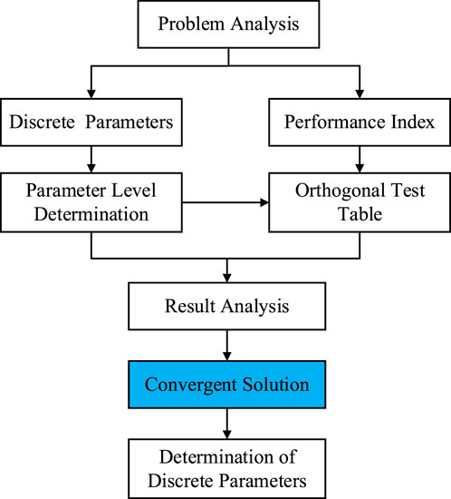
Figure 1. Procedure of the convergence study.

Based on the computational results, a critical step is to find the convergent solution of the problem. The convergent solution or optimal solution possesses distinct features. For instance, in many cases, the larger or the smaller the performance index, the better. For mechanical problems with discrete computational domains, in general, the performance index will gradually converge as the grid size decreases. In this work, this characteristic is utilized for determining the convergent solution. Based on the convergent solution, the performance index corresponding to the other discrete parameters can be further processed, and the optimal factor-level combination of the discrete parameters can be finally determined.

3 Results and discussions

3.1 Convergence study for the Kalthoff-Winkler experiment

The Kalthoff-Winkler experiment shown in Figure 2, which is a benchmark problem, has been investigated by many researchers. According to the references, the projectile is regard as a rigid body and the detailed parameters for the Kalthoff-Winkler experiment are given in Table 1. The thickness of the steel plate is 9 mm and all the boundaries are free. In addition, it should be noted that the initial velocity of the projectile and the fracture energy in Table 1 are slightly different from that in the actual experiment, and the difference is mainly to consider the influences of ignoring the projectile elasticity. The subsequent section provides a detailed discussion on how the fracture energy and the projectile initial velocity affect the crack propagation path.

Figure 2

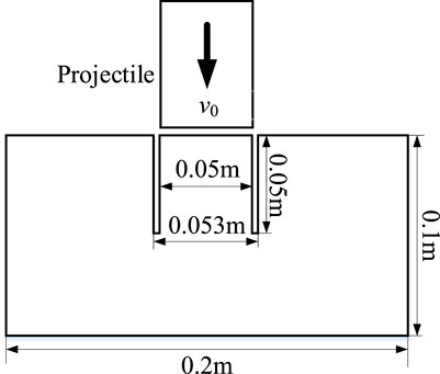
Figure 2. Setup of the Kalthoff-Winkler experiment.

Table 1

Table 1. Basic parameters for the Kalthoff-Winkler experiment.

The discretization of the computational domain of this problem mainly includes spatial discretization and temporal discretization. The spatial discretization is carried out in the form of a uniform discretization, which is characterized by $\Delta$, and the temporal discretization is characterized by ${\alpha }_t$ in Equation 10. The horizon $\delta =m\Delta$ is a core parameter for PD models, which determines the material points that participate in the integrations. Therefore, for this problem, we mainly conduct convergence investigations based on $\Delta$, m and ${\alpha }_t$. And the three factors are respectively referred to as A, B, and C in this work. At the initial moment, there is no strain distribution in the steel plate. Consequently, a parameter $k_{\text{DS}}$ defined in Equation 11 is a ratio between the elastic potential and the energy loss due to material damage, which can serve as the performance index in the convergence investigation.

$k_{\text{DS}}=\frac{E_{\mathrm{D}}}{E_{\mathrm{S}}}(11)$

where $E_{\mathrm{D}}$ is the energy loss due to material damage, and $E_{\mathrm{S}}$ is the elastic potential energy, i.e., the strain energy in the plate.

According to the procedure in Figure 1, factor levels should be determined before the orthogonal experiment design. The spatial discretization size is governed by the number of material points in the characteristic dimension orientation. For a problem with the characteristic length of 0.1 m, the length is uniformly discretized with 100 material points, and the corresponding spatial discretization size $\Delta$ is 1.0 mm. Generally, as the spatial discretization size decreases, the numerical calculation results will gradually converge. However, a small spatial discretization size can lead to excessive computational costs. Consequently, it is necessary to achieve a large spatial discretization size under the premise of result convergence. According to the existing literatures [27, 28], a spatial discretization size of 1.0 mm were utilized in there numerical predictions, and some researchers believe the spatial discretization size should reach 0.5 mm for achieving a convergent solution. In this work, we limit the spatial discretization size to between 0.4 and 0.7 mm.

As for factor B, which is parameter m, its values mainly range from 3.0 to 8.0 in PD models. The larger the parameter m, the more material points there are in the PD horizon of a material point, which will further lead to a sharp increase in the computational costs. Considering the computational cost and the parameter used in the existing literatures, parameter m in this work takes values between 3.0–6.0. As for parameter C, which defines the relationship between actual time step size used in the numerical predictions and the critical time step size. According to the requirements on the time step size, parameter ${\alpha }_t$ should be less than 1.0. And the specific value of factor C is limited to 0.2–0.8 in this work.

In order to obtain a convergent trend of the performance index, four levels were selected for each factor. The specific values of the three factors at different levels are given in Table 2. Based on the number of the factors and levels, the standard orthogonal test array L₁₆ (4⁵) was selected in the present work. It should be noted that the selected orthogonal array may vary depending on the problem at hand and the chosen number of levels. This significantly impacts the computational effort required to finalize the discrete parameters. For researchers with extensive experience, fewer levels may suffice to accurately pinpoint the optimal values. Based on this array, as illustrated in Table. 3, orthogonal experiments with up to 5 factors can be studied simultaneously, and a total of 16 sets of numerical cases should be investigated. In this work, bond-based PD model with the constant modulus was utilized, and the ratios between the elastic potential and the energy loss for the 16 sets of cases were obtained and presented in the column of Table 3.

Table 2

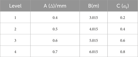
Table 2. Factor-levels.

Table 3

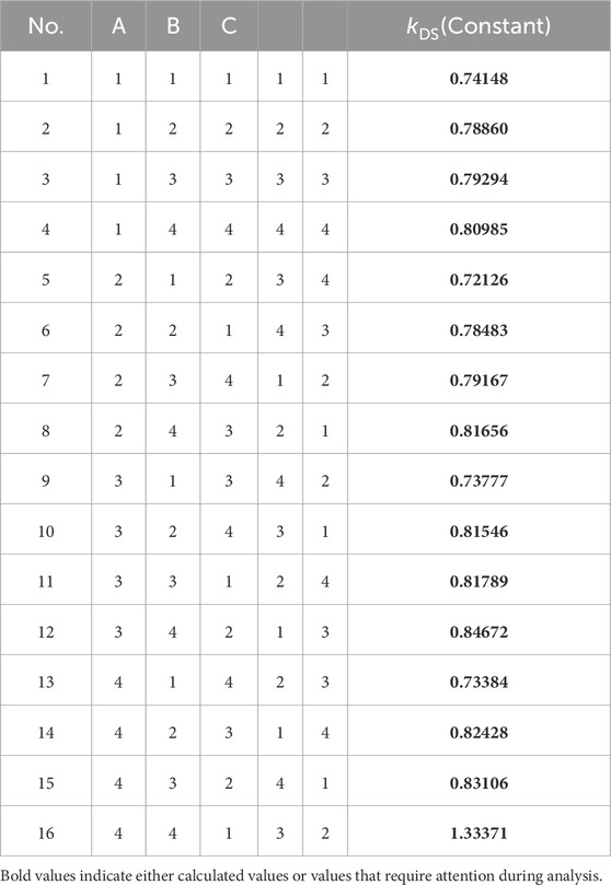
Table 3. L₁₆ (4⁵) orthogonal test array.

Based on the results in Table 3, detailed analyses of the performance index $k_{\text{DS}}$ are presented in Table 4. In the Table 4, B′ and C′ represent the performance results of factor B and factor C after processing based on the convergence solution, respectively. The processing was carried out based on Equation 12. K_ij is the summation of the performance index and ${\overline{K}}_{ij}$ is the averaged performance index under level i of factor j. $R_j$ and $R_j^{\prime }$ are the range and the normalized range of the averaged performance index of factor j, respectively. The two ranges are defined in Equation 13 and Equation 14, respectively. The normalized range effectively neutralizes unit-induced comparability issue among the factors.

$k^{\prime }=\left|k_{\text{DS}}-k_{\text{cv}}\right|(12)$

$R_j=\max \left({\overline{K}}_{1j},{\overline{K}}_{2j},{\overline{K}}_{3j},{\overline{K}}_{4j}\right)-\min \left({\overline{K}}_{1j},{\overline{K}}_{2j},{\overline{K}}_{3j},{\overline{K}}_{4j}\right)(13)$

$R_j^{\prime }=\frac{R_j}{\Delta F_j}(14)$

where $k_{\text{cv}}$ is the convergent numerical solution, which is obtained according the theoretical analysis of results following the convergence investigation procedure shown in Figure 1; $\Delta F_j$ is the normalized interval of factor j, which is a ratio between the level interval and the total range of the values of factor j, the corresponding expression is given in Equation 15.

$\Delta F_j=\frac{F_j^{\max }-F_j^{\min }}{n_j\left(F_j^{\max }-F_j^{\min }\right)}=\frac{1}{n_j}(15)$

where, $F_j^{\max }$ and $F_j^{\min }$ are the maximum level and the minimum level of factor j, respectively; $n_j$ is the number of levels of factor j. It should be noted that this formula is practically meaningful only when the factors have different numbers of levels.

Table 4

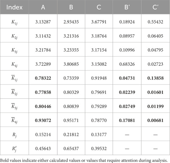
Table 4. Result analysis of the performance index.

In the field of computational mechanics, it is well known that the numerical solutions gradually converge as the spatial discretization size decreases. We utilized this characteristic to search for the convergent solution for the problem, and the results are presented in Figure 3. As shown in Figure 3a, the numerical results conform to the aforementioned laws of computational mechanics, and numerical results of the studied problem convergent when the spatial discretization size decreased to 0.5 mm, which is the second level of factor A. In this work, the convergent numerical solution $k_{\text{cv}}$ in Equation 12 is calculated by averaging the performance index of factor A at levels 1 and 2. Based on the convergent solution, the absolute residuals of the performance index for factor B and factor C can be achieved based on Equation 12. The absolute residuals are presented in Figures 3b,c. For the two parameters, obviously, the smaller the absolute residual, the better. According to Figure 3b, the optimal solution for parameter m is 4.015, which is the second level of factor B. According to Figure 3c, within the range of factor C, a value of ${\alpha }_t$ within 0.4–0.8 can obtain relatively accurate calculation results. Therefore, for the studied problem, the optimal discrete parameter combination is obtained. It should be noted that the results in Figure 3c are primarily related to the treatment of bond breaking processes. When the time step is very small, corrections must be made to bond fractures from the perspectives of momentum and energy conservation.

Figure 3

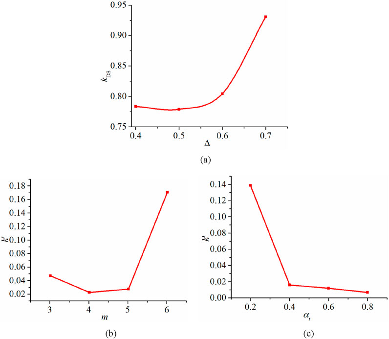
Figure 3. Convergence results. (a) Performance index vs. factor A. (b) The absolute residual k’ of factor B. (c) The absolute residual k’ of factor C.

The main purpose of the range analysis in Table 4 is to obtain the order of sensitivity of calculation results to the parameter changes. Obviously, the greater the range, the stronger the sensitivity. For the studied problem and within the selected ranges of the parameters, we found that the specific sensitivity order is: m> $\Delta$ >${\alpha }_t$.

Based on the optimal discrete parameter combination, a case of the Kalthoff-Winkler experiment was calculated. Detailed results are illustrated in Figure 4. The total energy in the plate comes from the kinematic energy of the projectile. Therefore, the consistency between the projectile energy loss and total energy within the steel plate shown in Figure 4a indicates the correctness of the energy balance in the system. According to Figure 4b, the projectile kinematic energy is converted into the elastic potential energy in the plate firstly. With the accumulation of the elastic potential energy, bond breakages occur and part of the potential energy is converted into the damage energy, which forms new surfaces of the cracks. Under the chain effect within the system, the elastic potential energy gradually decreases after the material damage starts. As illustrated in Figure 4c, the velocity of the projectile decreased from 16.5 m/s to 7.64 m/s during the interaction between the projectile and the steel plate. The damage and displacement distributions at 90 are given in Figures 4e,f. It should be noted that, the X-direction is consistent with the direction of the projectile impact, and the Y-direction is perpendicular to the direction of the projectile initial velocity. The cracks propagate at an angle of about 68° with respect to the direction of pre-notches, which agree with the numerical results in those works and experiments [27, 28].

Figure 4

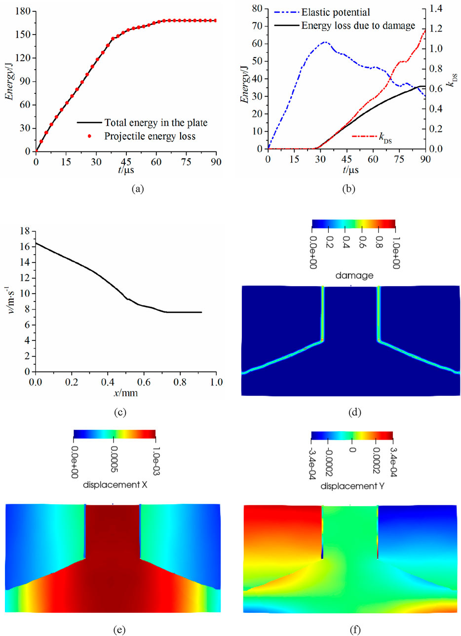
Figure 4. Numerical results of the Kalthoff-Winkler experiment. (a) Energy balance in the system. (b) Elastic potential and damage energy. (c) Projectile velocity vs. travel. (d) Damage at 90 μs. (e) X-displacement at 90 μs. (f) Y-displacement at 90 μs.

Figure 5

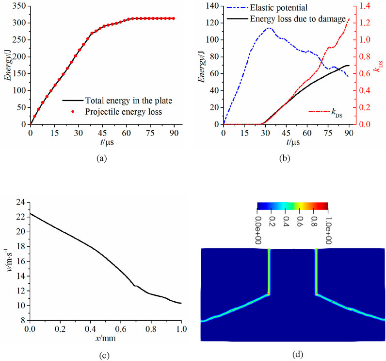
Figure 5. Improved numerical results of the Kalthoff-Winkler experiment. (a) Energy balance. (b) Elastic potential and damage energy. (c) Projectile velocity vs. its travel. (d) Damage distribution at 90 μs.

3.2 Discussions

An issue that worth further investigation is ensuring the consistency of basic conditions in numerical calculations and experiments of the benchmark problem. The plate is made of X2 NiCoMo 1895, which is a material similar to the standard grade 18Ni(300) [26]. The fracture toughness of the material is about 90 $\text{MPa}·{\mathrm{m}}^{1/2}$ [30], and the elastic modulus and the Poisson’s ratio are given in Table 1. Based on the material properties, the real fracture energy $G_{\mathrm{c}}$ can be calculated according to Equation 16 [31]. The result of the fracture energy is 42.408 kJ/m², which is different from the fracture energy in Table 1.

$G_{\mathrm{c}}=\left\{\begin{array}{l}\frac{1}{E}{K}^2\text{\hspace{1em}\hspace{1em}\hspace{1em}\hspace{1em}\hspace{1em}plane stress}\\ \frac{1-{\upsilon }^2}{E}{K}^2\text{\hspace{1em}\hspace{1em}\hspace{1em}\hspace{1em}\hspace{1em}plane strain}\end{array}\right.(16)$

where $\upsilon$ is Poisson’s ratio, E is the elastic modulus and K is the fracture toughness.

Another topic worth discussing is the initial velocity of the projectile. In many works [14, 27, 28], the interaction between the projectile and the steel plate is achieved through a fixed velocity boundary condition given at the contact boundary, and the given velocity is 16.5 m/s. However, a constant velocity boundary condition will affect the energy conversion in the actual process and cannot truly depict the projectile-plate interaction. In addition, the specific speed is mainly considered to maintain consistency between the required time of complete fracture of the steel plate in numerical calculations and the corresponding time in experiments. In the present work, we directly considered the impact between the projectile and the steel plate, but the projectile was treated as a rigid body. Similar to the considerations in the cases that maintain the temporal synchronization observed in numerical-experimental correlations, by trial and error, we have calculated that when the initial velocity of the projectile is 22.5 m/s, the time for the crack to completely penetrate the plate is about 90 microseconds, which is equal to the corresponding time recorded in the experiments [28, 32]. Based on parameters and basic conditions closer to the experimental situation, the Kalthoff-Winkler experiment was investigated by using the bond-based PD model and the discrete parameters obtained in Section 3.1.

Detailed results were illustrated in Figure 5. The numerical results are similar to those under initial impact velocity of 16.5 m/s, but the specific values vary significantly. For example, the total energy in the steel plate in Figure 5a reaches about 313.2 J, while the total energy in Figure 4a is about 170.0 J. And the total energy loss due to damage shown in Figure 5b is about 69.5 J, while the corresponding value in Figure 4b is about 35.8 J. This is mainly due to the increase in the fracture energy. As shown in Figure 5c, during the impact process between the projectile and the steel plate, the velocity of the projectile decreased from 22.5 m/s to 10.36 m/s. And the displacement of the projectile at 90 microseconds is about 1.16 mm. The damage distribution in the deformed configuration is given in Figure 5d, and the crack paths is similar to the crack propagation path in Figure 4d.

In Figure 6, the simulated crack path is compared with the path obtained from experiments. Different from the result in Figure 5d, the numerical result in Figure 6 is displayed in the referenced configuration. The experimental results and numerical calculations have a high degree of consistency, especially the crack initiation and the final fracture morphology. It should be acknowledged that the propagation path of the crack is slightly different. We believe that the main reason is the inherent fixed Poisson’s ratio defect in bond-based PD models.

Figure 6

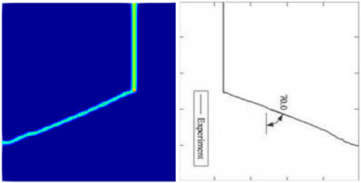
Figure 6. Simulated vs. experimental [32] crack propagation path.

4 Conclusion

In the present work, we proposed a novel method for verifying the discrete parameter independence of numerical results from bond-based PD models. The core of the method is to treat the discrete parameters as factors and utilize the advantages of orthogonal experimental design in comprehensive analysis, then the variation of numerical results with individual factors can be obtained. Furthermore, using the consensus in computational mechanics, that is, the numerical results will gradually converge with the discretization of spatial discretization size, and a convergent solution will be obtained. Based on the convergent solution, the optimal level of the other parameters can be obtained. Based on the method, the Kalthoff-Winkler experiment was studied and discussed in detail. Based on the result analysis and discussions, following conclusions can be drawn.

1. The proposed discrete parameter independence verification methodology demonstrates robust effectiveness, which provides theoretical and technical support for determining discrete parameters in numerical simulations.

2. For the Kalthoff-Winkler experiment, the discrete parameter values that can ensure the convergence of the numerical results are: $\Delta$ =0.5 mm, m=4.015 and ${\alpha }_t\in \left[0.4,0.8\right]$. For this issue, the bond-based PD simulations exhibit highest sensitivity to the variation of parameter m among the studied discretization parameters, and the sensitivity order is: m>$\Delta$>${\alpha }_t$.

3. In the Kalthoff-Winkler experiment, when directly considering the interaction between the projectile and the steel plate and the projectile is simplified as a rigid body, it is found that an initial velocity of 22.5 m/s exactly meets the requirement of the temporal synchronization observed in numerical-experimental correlations, and the calculated crack paths is highly consistent with the experimental results.

Data availability statement

The raw data supporting the conclusions of this article will be made available by the authors, without undue reservation.

Author contributions

CH: Conceptualization, Data curation, Funding acquisition, Methodology, Software, Validation, Writing – original draft, Writing – review and editing. XC: Conceptualization, Supervision, Validation, Writing – review and editing.

Funding

The author(s) declare that financial support was received for the research and/or publication of this article. We are grateful for the financial support from the National Natural Science Foundation of China (Grant No. 12202167), and the Natural Science Foundation of Jiangsu Province (Grant No. BK20210872).

Conflict of interest

The authors declare that the research was conducted in the absence of any commercial or financial relationships that could be construed as a potential conflict of interest.

Generative AI statement

The author(s) declare that no Generative AI was used in the creation of this manuscript.

Any alternative text (alt text) provided alongside figures in this article has been generated by Frontiers with the support of artificial intelligence and reasonable efforts have been made to ensure accuracy, including review by the authors wherever possible. If you identify any issues, please contact us.

Publisher’s note

All claims expressed in this article are solely those of the authors and do not necessarily represent those of their affiliated organizations, or those of the publisher, the editors and the reviewers. Any product that may be evaluated in this article, or claim that may be made by its manufacturer, is not guaranteed or endorsed by the publisher.

References

1. Macia F, Merino-Alonso PE, Souto-Iglesias A. On the convergence of the solutions to the integral SPH heat and advection-diffusion equations: theoretical analysis and numerical verification. Comput Methods Appl Mech Eng (2022) 397:115045. doi:10.1016/j.cma.2022.115045

CrossRef Full Text | Google Scholar

2. Kiran R, Khandelwal K. On the application of multipoint root-solvers for improving global convergence of fracture problems. Eng Fract Mech (2018) 193:77–95. doi:10.1016/j.engfracmech.2018.02.031

CrossRef Full Text | Google Scholar

3. Sepasdar R, Shakiba M. Overcoming the convergence difficulty of cohesive zone models through a newton-raphson modification technique. Eng Fract Mech (2020) 233:107046. doi:10.1016/j.engfracmech.2020.107046

CrossRef Full Text | Google Scholar

4. Rafaqat K, Naeem M, Akgul A, Hassan AM, Abdullah FA, Ali U. Analysis and numerical approximation of the fractional-order two-dimensional diffusion-wave equation. Front Phys (2023) 11:1199665. doi:10.3389/fphy.2023.1199665

CrossRef Full Text | Google Scholar

5. Zhang L, Wang FZ, Zhang J, Wang YY, Nadeem S, Nofal TA. Novel numerical method based on the analog equation method for a class of anisotropic convection-diffusion problems. Front Phys (2022) 10:807445. doi:10.3389/fphy.2022.807445

CrossRef Full Text | Google Scholar

6. Silling SA. Reformulation of elasticity theory for discontinuities and long-range forces. J Mech Phys Sol (2000) 48:175–209. doi:10.1016/S0022-5096(99)00029-0

CrossRef Full Text | Google Scholar

7. Bobaru F, Hu W. The meaning, selection, and use of the peridynamic horizon and its relation to crack branching in brittle materials. Int J Fract (2012) 176:215–22. doi:10.1007/s10704-012-9725-z

CrossRef Full Text | Google Scholar

8. Hu X, Li S. On nonlocal-deformation-field-driven bond-based peridynamics and its inherent nonlocal continuum mechanics. Comput Methods Appl Mech Eng (2025) 435:117593. doi:10.1016/j.cma.2024.117593

CrossRef Full Text | Google Scholar

9. Lian H, Zhao P, Zhang M, Wang P, Li Y. Physics informed neural networks for phase field fracture modeling enhanced by length-scale decoupling degradation functions. Front Phys (2023) 11:1152811. doi:10.3389/fphy.2023.1152811

CrossRef Full Text | Google Scholar

10. Shojaei A, Mudric T, Zaccariotto M, Galvanetto U. A coupled meshless finite point/Peridynamic method for 2D dynamic fracture analysis. Int J Mech Sci (2016) 119:419–31. doi:10.1016/j.ijmecsci.2016.11.003

CrossRef Full Text | Google Scholar

11. Bie YH, Liu ZM, Yang H, Cui XY. Abaqus implementation of dual peridynamics for brittle fracture. Comput Methods Appl Mech Eng (2020) 372:113398. doi:10.1016/j.cma.2020.113398

CrossRef Full Text | Google Scholar

12. Guo L, Bi C. Adaptive finite element method for nonmonotone quasi-linear elliptic problems. Comput Math With Appl (2021) 93:94–105. doi:10.1016/j.camwa.2021.03.034

CrossRef Full Text | Google Scholar

13. Beckmann R, Mella R, Wenman MR. Mesh and timestep sensitivity of fracture from thermal strains using peridynamics implemented in abaqus. Comput Methods Appl Mech Eng (2013) 263:71–80. doi:10.1016/j.cma.2013.05.001

CrossRef Full Text | Google Scholar

14. Ren H, Zhuang X, Rabczuk T. Dual-horizon peridynamics: a stable solution to varying horizons. Comput Methods Appl Mech Eng (2017) 318:762–82. doi:10.1016/j.cma.2016.12.031

CrossRef Full Text | Google Scholar

15. Bobaru F, Yang M, Alves LF, Silling SA, Askari E, Xu J. Convergence, adaptive refinement, and scaling in 1D peridynamics. Int J Numer Methods Eng (2009) 77:852–77. doi:10.1002/nme.2439

CrossRef Full Text | Google Scholar

16. Wu F, Bai M, Duan Q. A three-dimensional consistent ordinary state-based peridynamic formulation with high accuracy. Eng Anal Bound Elem (2024) 165:105758. doi:10.1016/j.enganabound.2024.105758

CrossRef Full Text | Google Scholar

17. Gong Y, Peng Y, Gong S. Symplectic time-domain finite element method for solving dynamic impact and crack propagation problems in peridynamics. Eng Anal Bound Elem (2025) 172:106119. doi:10.1016/j.enganabound.2025.106119

CrossRef Full Text | Google Scholar

18. Yu X-L, Zhou X-P. A nonlocal energy-informed neural network for peridynamic correspondence material models. Eng Anal Bound Elem (2024) 160:273–97. doi:10.1016/j.enganabound.2024.01.004

CrossRef Full Text | Google Scholar

19. Tong Q, Li S. Multiscale coupling of molecular dynamics and peridynamics. J Mech Phys Sol (2016) 95:169–87. doi:10.1016/j.jmps.2016.05.032

CrossRef Full Text | Google Scholar

20. Ha YD, Bobaru F. Studies of dynamic crack propagation and crack branching with peridynamics. Int J Fract (2010) 162:229–44. doi:10.1007/s10704-010-9442-4

CrossRef Full Text | Google Scholar

21. Ryono K, Ishioka K. New numerical methods for calculating statistical equilibria of two-dimensional turbulent flows, strictly based on the miller-robert-sommeria theory. FLUID Dyn Res (2022) 54:055505. doi:10.1088/1873-7005/ac9713

CrossRef Full Text | Google Scholar

22. Chen P, Guilleminot J. Spatially-dependent material uncertainties in anisotropic nonlinear elasticity: stochastic modeling, identification, and propagation. Comput Methods Appl Mech Eng (2022) 394:114897. doi:10.1016/j.cma.2022.114897

CrossRef Full Text | Google Scholar

23. Jiang Y, Li H, Jia H. Aerodynamics optimization of a ducted coaxial rotor in forward flight using orthogonal test design. Shock Vib (2018) 2018:2670439. doi:10.1155/2018/2670439

CrossRef Full Text | Google Scholar

24. Tang L, Yuan S, Tang Y. Performance improvement of a micro impulse water turbine based on orthogonal array. Math Probl Eng (2017) 2017:5867101. doi:10.1155/2017/5867101

CrossRef Full Text | Google Scholar

25. Diehl P, Prudhomme S, Lévesque M. A review of benchmark experiments for the validation of peridynamics models. J Peridynamics Nonlocal Model (2019) 1:14–35. doi:10.1007/s42102-018-0004-x

CrossRef Full Text | Google Scholar

26. Joerg FK. Modes of dynamic shear failure in solids. Int J Fract (2000) 101:1–31. doi:10.1023/A:1007647800529

CrossRef Full Text | Google Scholar

27. Guo JS, Gao WC. Study of the kalthoff–winkler experiment using an ordinary state-based peridynamic model under low velocity impact. Adv Mech Eng (2019) 11:1687814019852561–11. doi:10.1177/1687814019852561

CrossRef Full Text | Google Scholar

28. Bautista V, Shahbazian B, Mirsayar M. A modified mixed-mode Timoshenko-based peridynamics model considering shear deformation. Int J Mech Sci (2025) 285:109802. doi:10.1016/j.ijmecsci.2024.109802

CrossRef Full Text | Google Scholar

29. Madenci E, Oterkus E. Peridynamic theory and its applications (2014). doi:10.1007/978-1-4614-8465-3

CrossRef Full Text | Google Scholar

30. Silling SA. Dynamic fracture modeling with a meshfree peridynamic code. Comput Fluid Solid Mech (2003). 2003:641–4. doi:10.1016/B978-008044046-0.50157-3

CrossRef Full Text | Google Scholar

31. Perez N. Materials science: theory and engineering (2024). doi:10.1007/978-3-031-57152-7

CrossRef Full Text | Google Scholar

32. Kalthoff JF, Winkler S. Failure mode transition at high rates of loading. In: CY Chiem, HD Kunze, and LW Meyer, editors Proceedings of the international conference on impact loading and dynamic behavior of materials. Bremen, Germany: Verlag. p. 185–95.

Google Scholar