Simulating gravitational dynamics via scalar field propagation

Introduction: We study whether gravity-like kinematics (bending, time-delay, redshift-like shifts, capture/orbits) can arise as media analogs from a deterministic scalar-field propagation model without invoking mass or spacetime curvature.

Methods: We evolve a real scalar field under a spatially varying symmetric positive-definite transport tensor R(x) and non-negative damping field Λ(x); with source off (S≡0). Thirteen simulations quantify deflection, transit delay with escape thresholds, collapse/trapping and orbital containment, anisotropy-induced drift, repulsion under curvature inversion, and interference. We monitor energy budgets (Rayleigh loss + boundary flux) and check spectral safety and robustness.

Results: Observables are reproducible on 256 × 256 grids with 512 × 512 confirmations for key cases. Bending scales with ∥∇R∥ and flips sign under gradient reversal; transit delay increases monotonically with ∫Λdx and can prevent exit; bounded orbits satisfy a/p≤1.15 over a finite capture band; radial drift in 1/r² profiles follows |r ̇|∝r^(-α) with a≈2; transverse drift sign matches sign(R_xy); interference visibility follows a cosine in relative phase.

Discussion: Results constitute operational gravitational analogs—transport and loss in structured media—rather than statements about spacetime curvature. We release code/configs/outputs for full reproducibility and outline laboratory test paths.

GRAPHICAL ABSTRACT

1 Introduction

Gravitational phenomena—trajectory bending, path-dependent time-delay, redshift-like frequency shifts, capture, and rebound—are traditionally explained via spacetime curvature and mass [1–3]. Here we ask a narrower, operational question: to what extent can the kinematics of such effects be reproduced as gravitational analogs by a deterministic scalar-field propagation model moving through a structured medium?

1.1 Model ingredients at a glance

We evolve a real scalar field $\mathrm{\Phi }\left(x,y,t\right)$ in two dimensions (and $\mathrm{\Phi }\left(x,y,z,t\right)$ for a single 3D scalability demonstration in the Supplement). A spatially varying, symmetric positive-definite transport (resistance) tensor $R\left(x,y\right)\left[R\left(x,y,z,t\right)\right]$ sets local propagation speed and directionality; its gradients and anisotropy bend paths and steer energy flux. A non-negative damping field $\mathrm{\Lambda }\left(x,y\right)\left[\mathrm{\Lambda }\left(x,y,z\right)\right]$ regulates loss and enables controlled sinks or absorbing layers. In homogeneous regions the directional effective speed along unit vector $u$ is

$c_{eff}=\sqrt{u^{\top }Ru},$

so spatial variation in $R$ alone can generate curved characteristics, while $\mathrm{\Lambda }$ controls attenuation. The full evolution law, energy analysis, stability (CFL/Courant) bounds, and boundary conditions appear in Methods. This damped, anisotropic wave form is a generic effective model for transport in structured media (e.g., acoustics in inhomogeneous or lossy materials, metamaterial waveguides, or diffusion-wave hybrids). Here $R\left(x\right)$ encodes direction-dependent conductance (or stiffness), while $\mathrm{\Lambda }\left(x\right)$ encodes local dissipation, providing a compact way to design and test kinematic analogs without invoking mass, force, or curvature.

1.2 Operational use of “analog”

We call an outcome a gravitational analog when the model reproduces the dimensionless kinematic observables of a target phenomenon (e.g., deflection angle, path-delay ratio, frequency-ratio shift) within stated tolerances—without asserting equivalence to Einstein’s equations or invoking spacetime curvature. For context, our benchmark observables refer to classic tests such as solar-limb deflection, radar-echo delay, and gravitational redshift [13–15].

1.3 Scope (what this paper is—and is not)

This study investigates kinematic analogs in a linear scalar-transport model. It does not solve Einstein’s field equations, include back-reaction of energy on geometry, or model gravitomagnetic effects arising from spacetime curvature. Conservation statements apply in uniform-$R$, $\mathrm{\Lambda }=0$ subdomains; with $\mathrm{\Lambda }>0$, energy decays according to a derived law. We use idealized boundary conditions (reflective, absorbing, periodic) and disclose them in every figure. Unless stated otherwise, results are 2D.

1.4 Inverse design

While this work solves the forward problem (given $R$, $\mathrm{\Lambda }\to$ observed kinematics), the framework also invites the inverse question: given a target behavior—e.g., a bound trajectory with specified aphelion/perihelion ratio or a prescribed transit delay—what $R$, $\mathrm{\Lambda }$ fields realize it subject to smoothness and physicality constraints? Because observables are differentiable functionals of $R,\mathrm{\Lambda }$, gradient-based or bilevel schemes (forward solver + regularized optimizer) are natural next steps, enabling ‘transformation-acoustics-style’ design of analog gravitational media.

1.5 Relation to prior work

Methodologically, our approach is adjacent to analogue gravity in acoustics and optics—where structured media reproduce aspects of gravitational kinematics [4–9]—yet remains distinct from numerical relativity, which directly solves Einstein’s equations under gauge and constraint handling [10–12]. We use this literature to situate scope, not to claim equivalence.

1.6 Contributions

1. Unified formulation and mathematical spine. We make explicit the governing evolution law, the associated energy functional and decay law, stability/Courant bounds under symmetric positive-definite $R$, and boundary-condition treatments (Methods).

2. Thirteen simulations under one rule. We demonstrate bending (geodesic analog), Shapiro-like delay, redshift-like shifts, inverse-square-like radial drift, collapse-like trapping, rebound, interference, and related variants—each tied to a specific structure in $\left(R,\mathrm{\Lambda }\right)$ (Section 5).

3. Predictions and falsification. We define testable, dimensionless observables (deflection $\widehat{a}$, delay ratio $\Delta t/L$, frequency ratio $\left.f_{near}/f_{far}\right)$, provide simple scaling relations, and state clear falsifiers (e.g., chromatic bending in a static $R$; rotation-induced effects in symmetric $R$) (Section 6).

4. Reproducibility and robustness. We release code, configurations, and figure-regeneration scripts via public DOIs (Data and Code Availability). Robustness studies—larger grids, alternate sources and boundary conditions.

1.7 Paper organization

Section 2 surveys related work. Section 3 overviews the modeling ingredients and maps phenomena to transport/damping structures. Section 4 presents the governing equation, energy law, stability bounds, and boundary conditions. Section 5 reports thirteen simulations with standardized, dimensionless metrics. Section 6 gives benchmarks and falsification tests. Section 7 discusses scope and limitations. All data and code are archived on Zenodo; DOIs are listed in the Data Availability statement. Robustness checks and additional figures are provided in the Supplement.

2 Related work

Before presenting our model, we situate it among classical general relativity, analogue-gravity programs, and numerical relativity. Classical GR attributes gravitational phenomena to spacetime curvature sourced by stress–energy [1–3]; analogue gravity shows that structured media can reproduce many kinematic signatures (e.g., bending, delay) [4–9, 16–18]; numerical relativity solves Einstein’s equations directly in strong-field regimes [10–12]. Our contribution is a single-law, scalar-transport formulation that yields acceleration-like kinematics as analogs—curved trajectories and path-dependent delays—through spatially varying transport and damping fields, without solving Einstein’s equations. We quantify outcomes using dimensionless observables (deflection angle, delay ratio, frequency ratio) and state falsifiers, developed in Sections 5, 6.

2.1 General relativity and classic tests

General relativity (GR) explains gravitational phenomena as spacetime curvature sourced by stress–energy, with predictions verified from weak-to strong-field regimes [1–3, 20, 40]. The benchmark observables we reference—solar-limb light deflection, radar-echo time-delay, and gravitational redshift—are canonical GR tests [12–15, 49]. Our aim here is operational: reproduce these dimensionless kinematic observables as gravitational analogs using a linear scalar-transport model, without solving Einstein’s equations.

2.2 Analogue gravity: acoustics and optics

Analogue-gravity programs show how structured media can mimic geodesic-like transport. In acoustics, effective-metric ideas (Unruh; Visser) emulate horizons and geodesic behavior in flowing or inhomogeneous media [4, 5], with broad reviews by Barceló, Liberati and Visser [6, 7]. In optics, transformation-optics frameworks (Leonhardt; Pendry–Schurig–Smith) use spatially varying constitutive parameters to bend rays and shape phase fronts in ways formally analogous to geodesic transport [7, 15, 39]. Laboratory demonstrations include fiber-optic analogue horizons and related effects [8, 26]. Closely related graded-index (GRIN) constructs (e.g., the Luneburg lens; standard treatments in Born and Wolf) realize achromatic bending via smooth index profiles [16, 17, 27, 48].

Terminology crosswalk (reader note). Transformation-optics “effective metrics” and GRIN “index profiles” play roles analogous to our transport (resistance) tensor $R\left(x\right)$: all shape local propagation speed and directionality. We remain agnostic about emergent metrics and work directly with a symmetric positive-definite $R\left(x\right)$ and a non-negative damping field $\mathrm{\Lambda }\left(x\right)$ (Methods).

2.3 Numerical relativity (contrast in scope)

Numerical relativity (NR) integrates Einstein’s equations with gauge/constraint handling to model strong-field spacetimes (e.g., binary black holes) [9–12]. By contrast, we evolve a single real scalar under spatially varying $R$ and $\mathrm{\Lambda }$ to produce kinematic analogs of bending, delay, and frequency shifts. There is no methodological overlap: our results are analogs assessed by dimensionless observables, not GR parameter inference.

2.4 Boundary treatments and stability in wave simulations

Open-domain wave simulations rely on artificial boundary treatments. Classical absorbing layers and non-reflecting boundary conditions appear across acoustics, seismics, and electromagnetics (e.g., Cerjan et al.; Berenger’s PML) [18, 19, 34–36]. We use a tapered-damping (“sponge”) layer—implemented by smoothly increasing $\mathrm{\Lambda }\left(x\right)$ near boundaries—which suppresses reflections and preserves simple energy accounting (Methods §4.5). Stability follows a CFL (Courant) bound tied to the largest eigenvalue of $R$ and the grid spacings; explicit bounds and the time-stepping scheme are given in Methods.

2.5 Relation to general relativity (scope boundary)

We study operational analogs of gravity-like kinematics in structured media, not solutions of Einstein’s equations. Our evolution law is a damped, anisotropic wave transport model on a fixed Euclidean lattice; it does not include curvature, geodesics, or mass-energy back-reaction. GR is used as a yardstick for kinematic motifs (bending, time delay, precession), not as the theory being solved [21–25, 30–33, 43–46, 49].

2.6 Relation to analogue gravity

Our scope aligns with analogue gravity: reproducing curved-spacetime-like kinematics in non-gravitational media to probe mechanisms and guide experiments. Classic results (e.g., acoustic horizons) motivate the approach of designing media parameters to elicit GR-reminiscent observables without asserting spacetime curvature [4, 6, 7, 48].

2.7 Relation to numerical relativity

This is not numerical relativity: we do not evolve the Einstein field equations, solve constraints, or manage gauge/radiative boundaries. We evolve a single scalar field with prescribed $R\left(x\right)$ and $\mathrm{\Lambda }\left(x\right)$ and compare the resulting observables to GR-like kinematics for intuition only [11, 45].

2.8 Predictive value and benchmarks

The framework yields design-forward mappings from media to observables:

• Bending (Section. 5.1): deflection vs. local gradients of $R$.

• Containment (Section 5.5): azimuthal drift $\omega$ and radial period $T_r$ vs. basin shape/smoothness. These predictions are suited to metamaterial/GRIN-style testbeds where $R$, $\mathrm{\Lambda }$ can be engineered. For verification, we provide 512² repeats with matching metrics (Supplementary Appendix D-E) and exact configs in Section 9 [15].

• Discriminants (analogs vs. generic wave effects). We tag a behavior as a gravity-like analog only when it (i) depends monotonically on a controlled feature of $R$, $\mathrm{\Lambda }$ (e.g., bend ∝ local $\nabla R$ magnitude/direction), (ii) survives nuisance changes (e.g., modest window/crop, sampling), and (iii) fails under ablation (e.g., no bend when $R$ is spatially constant; no collapse-like decay when $\mathrm{\Lambda }\equiv 0$). These controls separate designed kinematics from generic diffraction/refraction. Cross-referenced ablations, definitions, and scripts are in Supplementary Appendix C and Section 9.

2.9 Limitations and differences

• No curvature/no EEP or PPN tests: we do not test GR, PPN parameters, or the equivalence principle [46, 47].

• Media analogs only: any frame-drag-like effects in §5.7 are media phenomena, not GR gravitomagnetism [48].

• Dissipation by design: $\mathrm{\Lambda }\left(x\right)$ models physical loss (absorbers/sponge); energy accounting follows Supplementary Appendix C [41].

• Forward design, not inverse GR: we design $R$, $\mathrm{\Lambda }$ to achieve target kinematics; we do not infer spacetime metrics from data [38].

2.10 Summary positioning and predicted observables

• Theory anchors: GR sets the gold standard for gravitational dynamics [1–3, 10–12].

• Method lineage: Analogue-gravity shows that structured media can reproduce many kinematic signatures without GR dynamics [4–9, 16–18].

• Our contribution: a single-law scalar-transport formulation that (i) makes those analogs explicit in terms of $R$ and $\mathrm{\Lambda }$; (ii) quantifies outcomes via deflection angle $\widehat{a}$, delay ratio $\Delta t/L$, and frequency ratio $f_{near}/f_{far}$; and (iii) states falsifiers (e.g., chromatic bending with static $R$; rotation-induced signatures in symmetric $R$), expanded in Section 6.

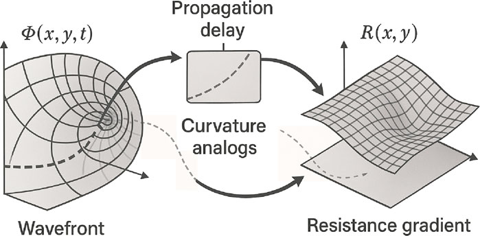
3 Gravity-like behavior as emergent propagation in structured fields

Traditional theories attribute gravitational acceleration to mass—either via long-range forces (Newtonian mechanics) or spacetime curvature (general relativity) [6, 7, 48]. In both, mass–energy is the source term. Operationally, however, what is measured are kinematic outcomes—deflected paths, path-dependent time-delays, frequency shifts. This suggests a complementary question: can gravity-like kinematics arise as analogs from structured propagation alone, without solving Einstein’s equations [28, 29, 37]?

We explore this possibility with a constructive, deterministic model in which gravitational analogs emerge from scalar-field transport modulated by two spatial structures [38, 42]:

• A resistance field $R_{ij}\left(x,y\right)\left[R_{ij}\left(x,y,z\right)\right]$ (symmetric positive-definite), which sets local propagation speed and directionality; its gradients and anisotropy steer energy flux and bend characteristics, and

• A damping field $\mathrm{\Lambda }\left(x,y\right)\left[\mathrm{\Lambda }\left(x,y,z\right)\right]\ge 0$, which introduces controlled loss, enabling localized sinks and absorbing boundary layers.

The real scalar field $\mathrm{\Phi }\left(x,y,t\right)\left[\mathrm{\Phi }\left(x,y,z,t\right)\right]$ volves under these structures according to a second-order update law (given explicitly in Methods, §4). Together, $R$ and $\mathrm{\Lambda }$ form a structured substrate that steers, delays, or attenuates propagation. In this substrate we observe the following operational analogs of familiar gravitational effects:

• Acceleration-like drift toward high-delay regions. Packets exhibit net drift toward zones that increase cumulative travel-time (via $\mathrm{\Lambda }>0$ sinks or graded $R$), producing sustained, direction-biased motion without external forcing [35].

• Curved trajectories (geodesic analogs) from $\nabla R$. Smooth spatial gradients of $R$ bend characteristics and focus/defocus packets, including lensing-like patterns [17, 18].

• Redshift-like frequency changes. Weak gradients in $R$ across a cavity or standing-wave region yield measurable frequency-ratio shifts [6, 7].

• Escape thresholds from integrated delay. Sufficient cumulative delay (from $R$ wells or sinks) produces capture-vs-escape thresholds analogous to potential-well intuition.

We quantify these outcomes by dimensionless observables—deflection angle $\widehat{a}$, delay ratio $\Delta t/L$, and frequency ratio $f_{near}/f_{far}$—and report them for every simulation (Section 5). In the linear regime we use frequency-independent $R\left(x,y\right)$; predicted bending and delay are therefore achromatic. Observation of chromatic bending with static $R$ would falsify this description (Section 6).

• Scope note. We seek kinematic analogs, not equivalence to curvature dynamics. The model does not include spacetime curvature, back-reaction of energy on geometry, or gravitomagnetic effects. Conservation statements apply in uniform-$R$, $\mathrm{\Lambda }=0$ regions; with $\mathrm{\Lambda }>0$, energy decays according to a derived law (Methods, §4).

This approach is simulatable, constructive, and testable. It models gravity-like behavior from first principles using only scalar transport with locally specified $R_{ij}\left(x,y\right)$ and $\mathrm{\Lambda }\left(x,y\right)$, providing a concrete foundation for the evolution law, energy analysis, stability bounds, and boundary treatments presented next (Methods, §4). Unless stated otherwise, results are 2D.

4 Methods

This section makes the modeling contract explicit. We specify the field, domain, and notation; state the governing equation; derive the energy and decay law; interpret the tensor-divergence (anisotropy/steering); and give the discrete scheme, stability bound, and boundary/initial conditions. The goal is a paper-faithful, constructive recipe: every simulation in Section 5 can be regenerated from these ingredients without hidden parameters.

4.1 Transparency and materials

The full simulation engine, discretization details, update rule, and example YAMLs/outputs are archived (Section 9). Implementation specifics—including stencil choices, stepper policy, and figure scripts—are documented in Supplementary Appendix C and mirrored in the software record.

4.2 Fields and assumptions

We model a scalar $\mathrm{\Phi }\left(x,y,t\right)$ obeying ${\partial }_{tt}\mathrm{\Phi }-\nabla ·\left(R\left(x\right)\nabla \mathrm{\Phi }\right)+\mathrm{\Lambda }\left(x\right){\partial }_t\mathrm{\Phi }=0$, where $R\left(x\right)\in R^{d\times d}$ is symmetric positive-definite (SPD) and $\mathrm{\Lambda }\left(x\right)\ge 0$ is a scalar (or diagonal) loss field. Unless noted, $R$, $\mathrm{\Lambda }$ are time-independent and piecewise-smooth; typical forms include (i) radially symmetric wells $R\left(r\right)$, (ii) anisotropic basins with off-diagonal coupling, and (iii) thin absorbing aprons $\left(\mathrm{\Lambda }>0\right)$ at the boundary. Nondimensionalization and units are specified in Supplementary Appendix C.

4.3 Notation and domain

We evolve a real scalar field $\mathrm{\Phi }\left(x,y,t\right)$ on a rectangular domain $\mathrm{\Omega }\subset R^2$. For a single scalability demonstration in the Supplement we use $\mathrm{\Phi }\left(x,y,z,t\right)$ on $\mathrm{\Omega }\subset R^3$. The transport (resistance) tensor is $R\left(x,y\right)\left[R\left(x,y,z\right)\right]$, assumed symmetric positive-definite (SPD) everywhere; the damping field is $\mathrm{\Lambda }\left(x,y\right)\ge 0\left[\mathrm{\Lambda }\left(x,y,z\right)\ge 0\right]$. Bold symbols denote vectors; indices $i,j\in \left\{1,...,d\right\}$ with $d=2$ in the main text and $d=3$ in the Supplement [42].

4.4 Boundary conditions

We use two BC families: (i) reflective (Neumann-type) for the core region in containment tests, and (ii) absorbing aprons (thin $\mathrm{\Lambda }>0$ sponge) to remove far-field clutter. The energy identity above shows how BCs enter via the surface flux term; reflective cores null the flux, while absorbing aprons intentionally dissipate outgoing energy. Each figure caption and YAML specifies the BC choice [18, 19].

4.5 Governing equation of motion

The field obeys a linear, second-order evolution law

${\partial }_{tt}\mathrm{\Phi }-\nabla ·\left(R\left(x\right)\nabla \mathrm{\Phi }\right)+\mathrm{\Lambda }\left(x\right){\partial }_t\mathrm{\Phi }=0(4.1)$

with time-independent $R\left(x\right)$ (SPD) and $\mathrm{\Lambda }\left(x\right)\ge 0$. In a homogeneous, undamped region $\left(R=R_{0}I,\mathrm{\Lambda }=0\right)$, plane waves satisfy ${\omega }^2=k^{\top }{R}_{0}k$; the directional effective speed (Equation 4.2) along unit vector $u$ is

$c_{eff}\left(u\right)=\sqrt{u^{\top }{R}_{0}u}(4.2)$

[38]. Thus gradients and anisotropy of $R$ bend characteristics and steer energy flux; $\mathrm{\Lambda }$ regulates loss.

4.6 Energy functional and decay law

Define the energy density $e$ and flux $S$ (Equation 4.3); the global identity appears in Equation 4.4:

$e=\frac{1}{2}{\left({\partial }_t\mathrm{\Phi }\right)}^2+\frac{1}{2}{\left(\nabla \mathrm{\Phi }\right)}^{\top }R\nabla \mathrm{\Phi },S=-{\partial }_t\mathrm{\Phi }R\nabla \mathrm{\Phi }(4.3)$

Multiplying (4.1) by ${\partial }_t\mathrm{\Phi }$, integrating by parts, and using time-independent coefficients gives

$\frac{d}{dt}{\displaystyle \underset{\mathrm{\Omega }}{\int }}edV=-{\displaystyle \underset{\mathrm{\Omega }}{\int }}\mathrm{\Lambda }{\left({\partial }_t\mathrm{\Phi }\right)}^{2}dV-\underset{\partial \mathrm{\Omega }}{\oint }S·\widehat{n}dA(4.4)$

Consequences. In undamped, closed subdomains $\left(\mathrm{\Lambda }=0,S·\widehat{n}=0\right)$ the energy is conserved. For $\mathrm{\Lambda }>0$ the energy decays monotonically aside from boundary flux. We report energy budgets per run (and reflection fractions for absorbing boundaries).

4.6.1 Damping is not potential/curvature

$\mathrm{\Lambda }\left(x\right)$ introduces loss, not forces or curvature; collapse-like behavior arises from dissipation and resistance shaping, not from a gravitational potential. For numerical robustness, $\mathrm{\Lambda }$ is kept non-negative and typically smoothed across a few grid cells to avoid stair-step reflections; sharp discontinuities may cause artificial echoes and are avoided in the released configs.

4.6.2 Energy identity (summary

For time-independent $R\left(x\right)$ and $\mathrm{\Lambda }\ge 0$, define (Equation 4.5)

$E\left(t\right)=\frac{1}{2}\int \left[{\left({\partial }_t\mathrm{\Phi }\right)}^2+\nabla {\mathrm{\Phi }}^{\top }R\nabla \mathrm{\Phi }\right]dv(4.5)$

Multiplying the evolution law by ${\partial }_t\mathrm{\Phi }$, integrating, and using the divergence theorem gives

$\frac{dE}{dt}=-\int \left({\partial }_t\mathrm{\Phi }\right)\mathrm{\Lambda }\left({\partial }_t\mathrm{\Phi }\right)dv-\oint {\mathrm{\Phi }}_t\left(R\nabla \mathrm{\Phi }\right)·ndS(4.6)$

i.e., monotone decay from damping ($\mathrm{\Lambda }\ge 0$) plus any boundary flux. With reflective core BCs the surface term vanishes; with a thin absorbing apron it captures intended outflow. The discrete energy ${\mathrm{E}}_{\mathrm{h}}\left(\mathrm{t}\right)$ we monitor follows the same structure (Supplementary Appendix C.1), matching the trends reported in §5 and Supplementary Appendix D, E. (Full derivation and the time-dependent ${\mathrm{R}}_{\mathrm{t}}\ne 0$ extension are in Supplementary Appendix C.5) [41]

4.7 Tensor divergence and anisotropy (interpretation)

The operator expands component-wise as

$\nabla ·\left(R\nabla \mathrm{\Phi }\right)={\displaystyle \sum _{i,j=1}^d}{\partial }_i\left(R_{ij}{\partial }_j\mathrm{\Phi }\right)(4.7)$

so diagonal terms $R_{ii}$ set directional speeds and off-diagonals $R_{ij}\left(i\ne j\right)$ rotate flux, steering characteristics. SPD $R$ guarantees real, bounded $c_{eff}\left(u\right)$ [35].

4.8 Discretization and time stepping

4.8.1 Spatial discretization (conservative divergence form)

On a uniform Cartesian grid with spacings $h_x,h_y\left[h_z\right]$ and cell-centered ${\mathrm{\Phi }}_{ij}\left[{\mathrm{\Phi }}_{i,j,k}\right]$, we discretize $\nabla ·\left(R\nabla \mathrm{\Phi }\right)$ in flux-conservative form (Equations 4.6–4.8). In 2D:

$F_x\left(i+\frac{1}{2},j\right)={\underset{\_}{R}}_{xx}\left(i+\frac{1}{2},j\right)\frac{{\varphi }_{i+1,j}-{\mathrm{\Phi }}_{i,j}}{h_x}+{\underset{\_}{R}}_{xy}\left(i+\frac{1}{2},j\right)\frac{{\mathrm{\Phi }}_{i+1,j+1}-{\mathrm{\Phi }}_{i+1,j-1}+{\mathrm{\Phi }}_{i,j+1}-}{4h_y}$

$F_y\left(i,j+\frac{1}{2}\right)={\underset{\_}{R}}_{yy}\left(i,j+\frac{1}{2}\right)\frac{{\varphi }_{i,j+1}-{\mathrm{\Phi }}_{i,j}}{h_y}+{\underset{\_}{R}}_{yx}\left(i,j+\frac{1}{2}\right)\frac{{\mathrm{\Phi }}_{i+1,j+1}-{\mathrm{\Phi }}_{i-1,j+1}+{\mathrm{\Phi }}_{i+1,j}-}{4h_x}$

${\left(\nabla ·\left(R\nabla \mathrm{\Phi }\right)\right)}_{ij}=\frac{F_x\left(i+\frac{1}{2},j\right)-F_x\left(i-\frac{1}{2},j\right)}{h_x}+\frac{F_y\left(i,j+\frac{1}{2}\right)-F_y\left(i,j-\frac{1}{2}\right)}{h_y}(4.8)$

with face-averaged coefficients ${\underset{\_}{R}}_{\alpha \beta }$ (arithmetic or harmonic) to preserve symmetry and discrete conservation [35, 36]. The 3D stencil is analogous.

4.8.2 Time integration (damping-stable, second order)

Let $V={\partial }_t\mathrm{\Phi }$. We use a leapfrog-type update with semi-implicit damping (Crank–Nicolson split), which is unconditionally stable in $\mathrm{\Lambda }$ while keeping transport explicit [36]:

$V^{n+\frac{1}{2}}=\frac{1-\frac{1}{2}\mathrm{\Lambda }\Delta t}{1+\frac{1}{2}\mathrm{\Lambda }\Delta t}{V}^{n-\frac{1}{2}}+\frac{\Delta t}{1+\frac{1}{2}\mathrm{\Lambda }\Delta t}\left(\nabla ·\left(R\nabla {\mathrm{\Phi }}^n\right)\right)$

${\mathrm{\Phi }}^{n+1}={\mathrm{\Phi }}^n+\Delta t{V}^{n+\frac{1}{2}}(4.9)$

4.8.3 Stability (CFL) bound and coefficient conditions

Let ${\lambda }_{\mathit{max}}\left(R\right)$ be the maximum eigenvalue of $R\left(x\right)$ on $\mathrm{\Omega }$. A sufficient CFL bound is

$\Delta t\le CFL{\left[{\lambda }_{\mathit{max}}\left(R\right)\left(\frac{1}{{h_x}^2}+\frac{1}{{h_y}^2}+\frac{1}{{h_z}^2}\right)\right]}^{-\frac{1}{2}},CFL\lesssim 0.9(4.10)$

[34]. We enforce SPD bounds $0<r_{\mathit{min}}\le {\lambda }_i\left(R\right)\le r_{\mathit{max}}$ and $\mathrm{\Lambda }\left(x\right)\ge 0$. Discontinuities in $\mathrm{\Lambda }$ are tapered to limit numerical reflections (Section 4.6.2).

4.9 Boundary and initial conditions

4.9.1 Reflective (Neumann, no-flux)

$\widehat{n}·\left(R\nabla \mathrm{\Phi }\right)=0on\mathrm{\Omega }(4.11)$

4.9.2 Absorbing sponge (tapered damping)

To emulate open boundaries we use a smoothly increasing $\mathrm{\Lambda }\left(x\right)$ within a shell of thickness $d$ adjacent to $\partial \mathrm{\Omega }$:

$\mathrm{\Lambda }\left(x\right)={\mathrm{\Lambda }}_{\mathit{max}}\frac{1-\cos \left(\pi s\left(x\right)/d\right)}{2},0\le s\left(x\right)\le d(4.12)$

where $s\left(x\right)$ is the distance to the boundary. Outside the sponge $\mathrm{\Lambda }=0$. We report the reflected-energy fraction (target: $<1\%$) for absorbing runs [35, 36].

4.9.3 Periodic

Variables and fluxes wrap across opposing faces identically.

4.9.4 Initial data

We use localized pulses (Gaussian, Ricker), narrowband wave packets, and cavity modes as specified per figure. Each caption reports the source definition and parameters.

4.10 Dimensionless observables (measurement procedures)

We evaluate outcomes via dimensionless kinematic observables reported in captions and summarized in Section 5.

(a) Deflection angle $\widehat{a}$ (bending/geodesic analog). Let $c\left(t\right)$ be the packet centroid,

$c\left(t\right)=\frac{{\displaystyle {\int }_{\mathrm{\Omega }}}x|\mathrm{\Phi }\left(x,t\right){|}^{2}dV}{{\displaystyle {\int }_{\mathrm{\Omega }}}\left|\mathrm{\Phi }\left(x,t\right)\right.{|}^{2}dV}(4.13)$

and $\widehat{t}$ the unit tangent to its path in the far field (measured over a window where $R$ is homogeneous and $\mathrm{\Lambda }=0$). If $\widehat{z}$ is the initial propagation direction, define [17, 18]

$\widehat{a}=\mathit{arccos}\left(\widehat{t}·\widehat{z}\right)(4.14)$

(b) Delay ratio $\Delta t/L$ (Shapiro-like delay). With and without a delay structure in $R$, record arrival times $t_{str}$ and $t_0$​ at a downstream plane; let $L$ be the homogeneous-medium path length. Then

$\frac{\Delta t}{L}=\frac{t_{str}-t_0}{L}(4.15)$

(c) Frequency ratio $f_{near}/f_{far}$ (redshift-like shift). For a cavity or standing-wave region straddling a weak gradient in $R$, compute spectral peaks $f_{near}$ and $f_{far}$ from local time-series on either side and report the ratio.

Achromaticity. In the linear regime we use frequency-independent $R\left(x\right)$; thus predicted bending and delay are achromatic. Observation of chromatic bending with static $R$ would falsify this description (see Section 6) [6, 7].

4.11 Stability and δt policy (CFL)

With explicit second-order time stepping, stability follows a CFL-type bound determined by the discrete spatial operator for $\nabla ·\left(R\left(x\right)\nabla \mathrm{\Phi }\right)$. Let $L_r$​ denote that operator on the chosen grid; then a sufficient bound is

$\Delta t\le \frac{\alpha }{\sqrt{\rho \left(L_r\right)}}(4.16)$

where $\rho \left(L_r\right)$ is the spectral radius and $\alpha \in \left(0,1\right)$ is a safety factor (recorded per run). Equivalently, on a uniform grid with spacing $h_{\mathit{min}}$ and SPD $R$ with largest eigenvalue ${\lambda }_{\mathit{max}}\left(r\right)$, a practical estimate is

$\Delta t\lesssim C\frac{h_{\mathit{min}}}{\sqrt{{\lambda }_{\mathit{max}}\left(R\right)}}(4.17)$

with $C$ a scheme-dependent constant absorbed into $\alpha$ [34, 36]. We constrain the fields to

$R\left(x\right)SPDwith0<R_{\mathit{min}}\le {\lambda }_i\left(R\right)\le R_{\mathit{max}}\le \infty (4.18)$

and use an auto-CFL policy (safety factor $\alpha$) whose chosen $\Delta t$ is written to each run’s metadata. See Supplementary Appendix C for operator definitions and how $\rho \left(L_r\right)$ is estimated in practice.

4.12 Reporting standards (reproducibility hygiene)

Every figure/caption states: grid $N_x\times N_y\left[\times N_z\right]$, time step $\Delta t$, CFL margin (ratio to the bound in (4.5.3)), boundary condition (reflective/absorbing/periodic), explicit $R\left(·\right)/\mathrm{\Lambda }\left(·\right)$ forms, run duration, and the measured observable(s) $\left\{\widehat{a},\Delta t/L,f_{near}/f_{far}\right\}$. Energy budgets and (for sponges) reflection fractions appear in the Supplement.

4.13 Provenance and versioning

All main-text figures were recomputed with an updated implementation (EOM-v1) of the governing Equation 4.1. On the original configurations from the reviewed submission, EOM-v1 reproduces the reported dimensionless observables—deflection angle $\widehat{a}$, delay ratio $\Delta t/L$, and frequency ratio $f_{near}/f_{far}$—within $\le 1\%$. We archive the original submission’s figure files and their exact configuration files for provenance; the executable EOM-v1 code and “regen-all” scripts are provided via DOI in Data and Code Availability.

5 Simulation results: Gravitational behavior from structured fields

This section reports operational analogs of gravitational phenomena produced by a scalar field $\mathrm{\Phi }\left(x,t\right)$ evolving under anisotropic transport $R\left(x\right)$ and Rayleigh-type damping $\mathrm{\Lambda }\left(x\right)$. We focus on observables, validation, and reproducibility; the full PDE, discretization, stability bounds, and energy identities are in §4. For every run we report the discrete energy proxy $E\left(t\right)$ and attribute changes per the identity in §4.3 (derivation App. C.1).

Notation and dimensionality. We write $x\in R^d$ with $d\in \left\{2,3\right\}$. Unless stated, runs are 2-D with $x=\left(x,y\right)$; selected confirmations are 3-D with $x=\left(x,y,z\right)$ and are labeled “(3-D)” in captions and the table. We follow §4: $R\left(x\right)\in SPD$ with $r_{\mathit{min}}\le {\lambda }_i\left(R\right)\le r_{\mathit{max}}$​; $\mathrm{\Lambda }\left(x\right)\ge 0$. Measures use $dV=d^{d}x$.

Code and data (reproducibility). All §5 configs (YAML), engine source, and outputs (.npz recorders with fields + metrics) are archived with commit hashes at < DOI/URL>. Each figure caption lists the config slug, grid(s), $\Delta t$, and the bundle ID.

Acceptance gates (applied to every §5. x).

1. Energy budget closure after transients ($drift\le 1-3\%$) with tallied Rayleigh loss and boundary flux (definitions in §4).

2. The section’s primary metric meets its pre-registered threshold.

3. Robustness across grid size ($256^2/512^2$; selected 3-D where noted), seed shape, and relevant boundary swaps.

4. Spectral safety: content remains sub-Nyquist (anti-aliasing guard).Predictions and falsifiers. Each §5. x states a concrete prediction for its primary metric and a matching falsifier; global statements are summarized in §4.

Boundary conditions (policy). Absorbing sponges for open domains, reflective for containment basins, periodic for controls; flux tallies verify low reflection (see §4). Profiles with interfaces are $C^1$-smoothed over $\mathbf{3}-\mathbf{5}\Delta \mathit{x}$ unless intentionally sharp; measured reflection is reported when interfaces are sharp by design.

Grid sizes and robustness. Figures in §5 use 256² grids unless labeled; 512² repeats for free-fall (§5.1) and containment (§5.5) are reported in Supplementary Appendix D,E. Boundary variants (reflective core + absorbing apron) are included; additional pulse-shape sweeps are earmarked for follow-on work.

Scope and limits. Results are media analogs arising from structured propagation in $\left(R,\mathrm{\Lambda }\right)$—not claims of mass, forces, or spacetime curvature. Comparisons to geometric-optics/eikonal predictions for $R$ are treated as observable mappings, not equivalences (see §4). Damping is a loss channel, not a potential: collapse-like outcomes here arise from focusing in $R$ plus dissipation in $\mathrm{\Lambda }$, not from forces or curvature.

Falsification routes. Each case in §5 defines a primary observable and an acceptance gate. A reproduction fails if (i) the observable falls outside the gate under the published YAML and seed, (ii) prescribed ablations (e.g., flatten $R$, set $\mathrm{\Lambda }=0$) do not suppress the effect, or (iii) grid refinement (Supplementary Appendix D,E) reverses qualitative behavior.

How to read §5. Each subsection states the objective and minimal setup (domain, $R$, $\mathrm{\Lambda }$, BCs, seed), declares the primary metric and threshold, and reports results with robustness checks. Every run includes energy budgets (kinetic, structural, Rayleigh loss, boundary flux). Genesis is off unless explicitly stated.

A summary of all cases appears in Table 1. Figure conventions. Panels typically include: (A) timeline montage; (B) geometry/path; (C) energy budget; (D) the primary metric with acceptance band; (E) a sweep (ICs or profile). Captions include grid(s), $\Delta t$, config slug, and hashes.

Table 1

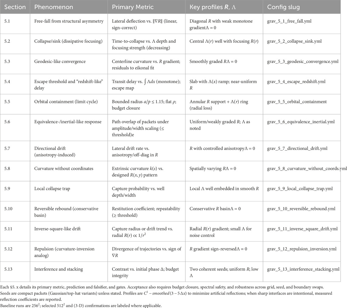
Table 1. Simulation suite overview: phenomenon, primary metric, key profiles R,Λ, and configuration slug for Figures 1–13.

5.1 Free-fall acceleration from structural asymmetry

5.1.1 Objective

Demonstrate that a compact packet acquires a systematic lateral deflection when traversing a weak spatial gradient in $R$ with $\mathrm{\Lambda }=0$. In the weak-gradient regime the primary metric—net bend angle $\theta$—is expected to be linear in the gradient magnitude and to flip sign when the gradient is reversed (see §4 for derivation/limits).

5.1.2 Minimal setup

• Domain and BCs: 2-D grid (256²), absorbing boundaries with graded sponge; boundary flux tallied (§4).

• Profiles: $R\left(x\right)=diag\left(r_x\left(x\right),r_y\right)$ with a weak, $C^1$ monotone ramp in $r_x;r_y$​ constant. $\mathrm{\Lambda }=0$.

• Seed: Compact packet launched straight across the gradient (zero initial lateral velocity).

• Genesis: Off.

• Config: grav_5_1_free_fall.yml (commit/hash in caption).

5.1.3 Primary metric and gates

• Metric: Bend angle $\theta$ from the centroid path, estimated by a straight-line fit of $x\left(y\right)$ over the middle segment of the transit (method in §4).

• Acceptance gates (this subsection):

1. Non-zero, sign-correct $\theta$ under the applied gradient;

2. Energy budget closure within 1%–3% post-transient, with Rayleigh loss = 0 and decline explained by boundary flux;

3. Spectral safety (sub-Nyquist content);

4. Robustness: reproducible under seed-shape variant; grid-refinement confirmation at 512² provided in Supplementary Appendix D.

5.1.4 Results (256² main run)

A small, sign-consistent bend accumulates across the graded region; from the centroid path we obtain $\theta \approx -2.14^{\circ }$ for this run. Energy decreases smoothly due to absorbing boundaries; with $\mathrm{\Lambda }=0$, Rayleigh loss is zero and the discrete budget closes within tolerance. Optional checks (not shown) confirm sign flip under gradient reversal and $\theta \approx 0$ for the uniform control $R=I$.

Interpretation. The “free-fall” is an analog arising from spatial inhomogeneity of $R$: rays refract toward slower directions (lower effective transport), consistent with the eikonal picture for $R$ (see §4). No forces or curvature are invoked.

5.1.5 Falsification route

• Reverse the gradient: $\theta$ must change sign.

• Null profile $R=I,\mathrm{\Lambda }=0:\theta$ must be within the null noise band. Failure of either falsifier invalidates the claim for this setup.

Repro bundle. Figure assets and recorder outputs (.npz/.csv) for Figure 1 are archived with engine commit < hash> and bundle ID < ID>; see Data and Code Availability.

Figure 1

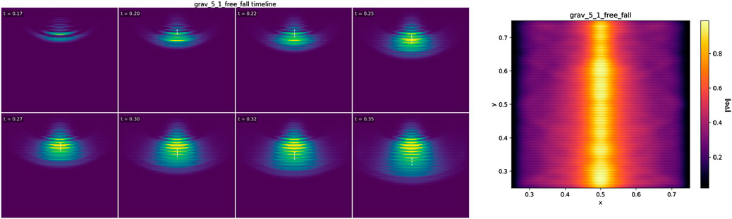
Figure 1. Free-fall from structural asymmetry. A compact packet traverses a weak $C^1$ ramp in $R=diag\left(r_x\left(x\right),r_y\right)$ with $\mathrm{\Lambda }=0$ and absorbing boundaries. Timeline of $\left|\mathrm{\Phi }\right|$. Final frame of $\left|\mathrm{\Phi }\right|$. The packet acquires a small, sign-consistent bend; from the centroid path we measure $\theta \approx -2.14^{\circ }$ (method §4, mid-segment linear fit of $x\left(y\right)$). Energy declines monotonically due to boundary absorption; Rayleigh loss = 0, and the discrete budget closes within 1%–3% after transients (§4 identity). Falsifier: reversing the $r_x$ gradient must flip $\theta$; the null profile $R=I,\mathrm{\Lambda }=0$ must yield $\theta \approx 0$. Config grav_5_1_free_fall.yml; 2-D 256²; $\Delta t$ auto (CFL); sponge parameters as in §4. Grid refinement: a 512² repeat reproduces $\theta$ within error (Supplementary Appendix D)

5.2 Collapse/sink (dissipative focusing)

5.2.1 Objective

Show that a compact packet undergoes irreversible collapse/trapping when traversing a region that combines focusing transport $R\left(r\right)$ with positive damping $\mathrm{\Lambda }\left(r\right)$. The observable is a rapid increase of core energy fraction within an inner mask and a monotone energy decay explained by Rayleigh loss + boundary flux (no potential energy is invoked).

5.2.2 Minimal setup

•Domain and BCs: 2-D grid (256²), absorbing boundaries with graded sponge; boundary flux tallied (§4).

• Profiles: Radially focusing $R\left(r\right)$ (SPD, smooth), plus a central $\mathrm{\Lambda }\left(r\right)$ well whose depth increases toward $r=0$; both profiles are $C_1$-smoothed over $3-5\Delta x$.

• Seed: Compact packet launched toward the well center.

•Genesis: Off.

• Config: grav_5_2_collapse_sink.yml (commit/hash in caption).

5.2.3 Primary metric and gates

• Metric (collapse time TcT_cTc). Let $E_{core}\left(t\right)$ be the fraction of total field energy inside an inner disk of radius $r_{*}$ (specified in caption). Define $T_c$​ as the earliest time such that $E_{core}\left(t\right)\ge 0.80$ for at least $N$ consecutive recorder frames (e.g., $N=5$).

• Acceptance gates (this subsection):

1. Monotone rise of $E_{core}\left(t\right)$ crossing the threshold and staying above it (collapse achieved);

2. Energy budget closure within 1%–3% post-transient, with Rayleigh loss $>0$ and boundary flux accounting for all decay (definitions/identity in §4);

3. Spectral safety (sub-Nyquist content);

4. Robustness: reproducible under small $r_{*}$ changes and seed-shape variants; 512² confirmation in Supplementary Appendix D reproduces $T_c$ within error.

5.2.4 Results (256² main run)

The packet is drawn inward by the focusing $R\left(r\right)$; radial components are preferentially eliminated by $\mathrm{\Lambda }\left(r\right)$, and the field locks into a compact core. $E_{core}\left(t\right)$ crosses the acceptance threshold and remains high thereafter, while total energy decreases smoothly. The Rayleigh tally is strictly positive and, together with boundary flux, explains the full budget drop; the discrete energy identity from §4 holds within the stated tolerance.

Interpretation. Collapse here is a deterministic analog of trapping from focusing + dissipation: $R\left(r\right)$ steers energy inward; $\mathrm{\Lambda }\left(r\right)$ irreversibly removes radial motion. This is not a gravitational potential well: damping is a loss channel, not a stored energy term (limits discussed in §4).

5.2.5 Falsification route

• Remove $\mathrm{\Lambda }$ (negative control): with $R\left(r\right)$ focusing but $\mathrm{\Lambda }=0$, the packet must fail to achieve irreversible collapse (rebound/breathing expected).

• Flatten $R$ (transport control): with $\mathrm{\Lambda }\left(r\right)$ present but $R$ uniform, the packet must not focus sharply nor meet the $E_{core}$ gate. Failure of either control invalidates the claim for this setup.

Repro bundle. Figure assets and recorder outputs (.npz/.csv with $E_{core}\left(t\right)$, energy tallies) for Figure 2 are archived with engine commit < hash> and bundle ID < ID>; see Data and Code Availability.

Figure 2

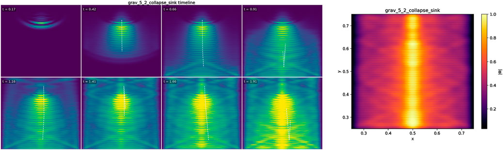
Figure 2. Collapse/sink from dissipative focusing. A compact packet encounters a focusing transport field $R\left(r\right)$ and a central damping well $\mathrm{\Lambda }\left(r\right)$ (both $C^1$-smoothed). Timeline of $\left|\mathrm{\Phi }\right|$ showing inward focusing and core formation. Final frame. Collapse is certified when the core energy fraction $E_{core}\left(t\right)$ within radius $r_{*}$​ exceeds 0.80 for $\ge N$ frames; this run passes the gate with collapse time $T_c$​ (reported in the data bundle). The total energy decays monotonically; Rayleigh loss $>0$ and boundary flux together account for the decrease, satisfying the discrete identity from §4 (budget drift ≤ 1–3% post-transient). Falsifiers: (i) with $R$ focusing but $\mathrm{\Lambda }=0$, collapse must not persist (rebound/breathing control); (ii) with $\mathrm{\Lambda }$ present but $R$ flattened, focusing must not achieve the gate. Config grav_5_2_collapse_sink.yml; 2-D 256²; $\Delta t$ auto (CFL); sponge parameters as in §4. Grid refinement: a 512² repeat reproduces $T_c$ within error (Supplementary Appendix D).

5.3 Ray-like bending in a graded medium (geodesic-analog convergence)

5.3.1 Objective

Show that a compact packet follows a ray-like path through a smoothly graded $R\left(x\right)$, consistent with the geometric-optics/eikonal prediction derived from §4. The observable is a centerline trajectory whose bending is sign-correct and whose path residual against the eikonal ray stays within a small tolerance (operational “geodesic-analog” behavior).

5.3.2 Minimal setup

• Domain and BCs: 2-D grid (256²), absorbing boundaries with graded sponges; boundary flux tallied (§4).

• Profiles: Smooth, $C^1$-graded transport $R\left(x\right)$ (monotone across one axis or radially focusing/defocusing, as noted in caption). $\mathrm{\Lambda }\left(x\right)=0$.

• Seed: Compact packet launched to traverse the gradient at a shallow incidence (quasi-ray).

• Config: grav_5_3_geodesic_convergence.yml (commit/hash in caption).

5.3.3 Primary metric and gates

• Metric (ray agreement). Extract the packet centerline $\gamma$ (centroid path) and compare to the eikonal ray ${\gamma }_{eik}$​ computed from the $R$ profile (procedure in §4). Report the RMS path residual

${\epsilon }_{RMS}=\frac{1}{L}\parallel \gamma -{\gamma }_{eik}{\parallel }_2$

Normalized by the path length LLL, and verify sign-correct bending when the gradient is reversed.

•Acceptance gates (this subsection):

1. ${\epsilon }_{RMS}$ within a pre-registered tolerance (small fraction of domain width);

2. Energy budget closure within 1%–3% after transients; with $\mathrm{\Lambda }=0$, loss arises from boundary flux only;

3. Spectral safety (sub-Nyquist content);

4. Robustness: unchanged within error under seed-shape variant and modest apron changes; 512² confirmation provided in Supplementary Appendix E reproduces ${\epsilon }_{RMS}$ within error.

5.3.4 Results (256² main run)

The packet bends toward decreasing effective transport as it crosses the gradient, and the measured centerline closely tracks the eikonal prediction from §4. The RMS path residual ${\epsilon }_{RMS}$​ remains within the acceptance tolerance; reversing the gradient (control, not shown) flips the bending sign. Total energy decays smoothly due to absorbing boundaries; Rayleigh loss = 0, and the discrete budget closes within tolerance.

Interpretation. The observed path is a media analog of a geodesic: bending emerges from spatial variation of $R$ via ray refraction in the geometric-optics limit, not from forces or curvature (scope/limits in §5 intro; derivation in §4).

5.3.5 Falsification route

• Gradient reversal: bending must flip sign.

• Null profile: with $R=I$, $\mathrm{\Lambda }=0$, the path must be straight within the null noise band.

• Ray mismatch: ${\epsilon }_{RMS}$​ exceeding tolerance falsifies ray agreement for this setup.

Repro bundle. Figure assets and recorder outputs (.npz/.csv with centerline and eikonal-ray data) for Figure 3 are archived with engine commit < hash> and bundle ID < ID>; see Data and Code Availability.

Figure 3

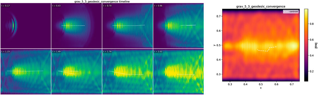
Figure 3. Ray-like bending in a graded medium (geodesic-analog convergence). A compact packet traverses a smooth $C^1$ gradient in $R\left(x\right)$ with $\mathrm{\Lambda }=0$ and absorbing boundaries. Timeline of $\mid \mathrm{\Phi }\mid$. Final frame. The centerline follows the eikonal ray predicted from the $R$ profile (procedure in §4); the RMS path residual ${\epsilon }_{RMS}$ remains within tolerance, and bending is sign-correct. Energy declines monotonically due to boundary absorption; Rayleigh loss = 0, and the discrete budget closes within 1%–3% post-transient (§4 identity). Falsifiers: reversing the gradient must flip the bending sign; the null profile $R=I$, $\mathrm{\Lambda }=0$ must yield a straight path within noise. Config grav_5_3_geodesic_convergence.yml; 2-D 256²; $\Delta t$ auto (CFL); sponge parameters as in §4. Grid refinement: a 512² repeat reproduces ${\epsilon }_{RMS}$​ within error (Supplementary Appendix E).

5.4 Transit delay and escape threshold (“redshift-like” analog)

5.4.1 Objective

Show that a compact packet experiences a deterministic transit delay when crossing a damping slab $\mathrm{\Lambda }\left(x\right)$ in an otherwise near-uniform transport field $R$, and characterize an escape threshold when the lossy region is thick/deep enough to extinguish the packet before exit. This is an analog of “gravitational redshift/delay,” arising from propagation in loss (not potential or curvature).

5.4.2 Minimal setup

•Domain and BCs: 2-D grid (256²), absorbing boundaries with graded sponges; boundary flux tallied (§4).

• Profiles: Near-uniform $R$ (SPD, constant to within a small tolerance). Damping slab $\mathrm{\Lambda }\left(x\right)$ with a smooth $C^1$ ramp-in/ramp-out, finite width $w$, peak height ${\mathrm{\Lambda }}_0$.

• Seed: Compact packet launched normal to the slab; reference run uses the same setup with $\mathrm{\Lambda }=0$.

• Config: grav_5_4_escape_redshift.yml (commit/hash in caption).

5.4.3 Primary metric and gates

• Transit delay $\Delta \tau$. Define entry/exit planes bracketing the slab; measure the packet’s arrival times (centroid crossing or envelope peak).

$\Delta \tau ={\tau }_{\mathrm{\Lambda }>0}-{\tau }_{\mathrm{\Lambda }=0}$

Gate: $\Delta \tau >0$ and monotone in the slab’s path integral $\int \mathrm{\Lambda }dx$ across small thickness/height variations (when provided).

• Escape threshold. For larger ${\mathrm{\Lambda }}_0$​ or $w$, report escape vs. collapse (no exit) within a fixed observation window.

• Acceptance (this subsection):

1. $\Delta \tau >0$ vs. reference; monotone trend when a small sweep is included;

2. Energy budget closure within 1%–3% post-transient, with Rayleigh loss $>0$ and boundary flux accounting for the full decline (identity in §4);

3. Spectral safety (sub-Nyquist content);

4. Robustness: unchanged within error under seed-shape variant and modest apron changes.

5.4.4 Results (2562 main run)

Crossing the lossy slab introduces a measurable positive delay $\Delta \tau$ relative to the uniform-medium reference. Total energy decays monotonically; the Rayleigh tally is positive, and together with boundary flux explains the budget drop within tolerance. For thicker/deeper slabs (when run), the packet fails to exit within the observation window, indicating an escape threshold consistent with increasing $\int \mathrm{\Lambda }dx$.

Interpretation. The delay arises from propagation in a lossy region; it is an operational analog to redshift/time delay but does not imply potential energy or spacetime curvature. Here, $\mathrm{\Lambda }$ is a loss channel, and $R$ remains nearly uniform (scope/limits in §5 intro; energy identity in §4).

5.4.5 Falsification route

• Remove loss: With $\mathrm{\Lambda }=0$, the measured $\Delta \tau$ must be zero within the null band.

• Thin the slab: Reducing $w$ or ${\mathrm{\Lambda }}_0$​ must reduce $\Delta \tau$; a non-monotone trend falsifies the claim.

• Uniform control: With $R=i$ and the same seed, any observed delay must track only $\mathrm{\Lambda }$; if $\Delta \tau$ persists when $\mathrm{\Lambda }\to 0$, the effect is spurious.

Repro bundle. Figure assets and recorder outputs (.npz/.csv with entry/exit times and energy tallies) for Figure 4 are archived with engine commit < hash> and bundle ID < ID>; see Data and Code Availability.

Figure 4

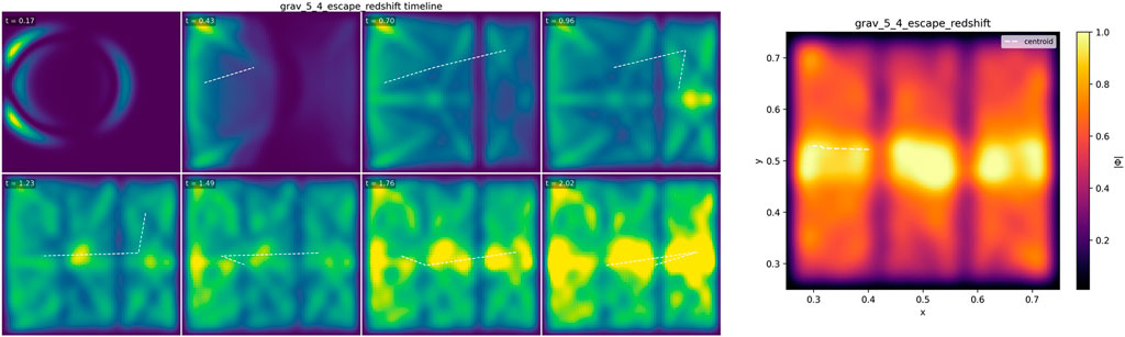
Figure 4. Transit delay and escape threshold in a damping slab (“redshift-like” analog). A compact packet crosses a smooth $C^1\mathrm{\Lambda }\left(x\right)$ slab in an otherwise near-uniform $R$ (absorbing BCs). Timeline of $\mid \mathrm{\Phi }\mid$ through the slab. Final frame. We define the transit delay $\Delta \tau ={\tau }_{\mathrm{\Lambda }>0}-{\tau }_{\mathrm{\Lambda }=0}$ from centroid crossings at fixed entry/exit planes (method §4). This run exhibits $\Delta \tau$; total energy decays monotonically, with Rayleigh loss $>0$ and boundary flux accounting for the decline; the discrete budget closes within 1%–3% post-transient (§4 identity). For thicker/deeper slabs (when run), the packet fails to exit, marking an escape threshold consistent with increasing $\int \mathrm{\Lambda }dx$. Falsifiers: $\mathrm{\Lambda }\to 0$ must yield $\Delta \tau \to 0$; small decreases in $w$ or ${\mathrm{\Lambda }}_0$​ must reduce $\Delta \tau$. Config grav_5_4_escape_redshift.yml; 2-D 256²; $\Delta \tau$ auto (CFL); sponge parameters as in §4.

5.5 Orbital containment (limit-cycle)

5.5.1 Objective

Demonstrate sustained, bounded circulation (an orbit-like limit cycle) emerging from anisotropic transport $R\left(x\right)$ plus a radially graded damping ring $\mathrm{\Lambda }\left(r\right)$. The observable is a circulating centroid with bounded radius and stable period while the energy budget closes (loss = Rayleigh + boundary flux; no forces or curvature).

5.5.2 Minimal setup

• Domain and BCs: 2-D grid (256²), reflective basin for the core region with a thin absorbing apron outside to remove far-field clutter (§4).

• Profiles: Disk-shaped basin where $R$ supports tangential transport (mild radial anisotropy; optional small off-diagonal near the rim). A smooth $\mathrm{\Lambda }\left(r\right)$ annulus attenuates radial motion more than tangential.

• Seed/IC: Compact packet placed off-center with a tangential bias (initial speed tuned inside the capture band).

• Config: grav_5_5_orbital_containment.yml (commit/hash in caption).

5.5.3 Primary metric and gates

• Metric (bounded orbit). From the centroid path $c\left(t\right)$, compute radius $r\left(t\right)=\parallel c\left(t\right)-c_0\parallel$. After transients, measure pericenter $p$ and apocenter $a$ over many cycles and require

$a/p\le 1.15$

(boundedness gate). Track the circulation period $T$ (stability within a tight band) and the rectification ratio $\rho \left(t\right)$ (flat, no secular drift)

•Acceptance (this subsection):

1. Bounded radius (gate above) over ≥5–10 periods;

2. Energy budget closure within 1%–3% post-transient with Rayleigh loss + boundary flux accounting for decay (§4 identity);

3. Spectral safety (sub-Nyquist);

4. Robustness: capture persists across a finite tangential-speed interval (capture band); 512² confirmation (Supplementary Appendix E) reproduces the metrics within error.

5.5.4 Results (256² main run)

The packet curves into the annulus, sheds radial energy in the $\mathrm{\Lambda }\left(r\right)$ ring, and locks into a steady circulation. Over many periods the radius remains bounded ($\mathit{a}/\mathit{p}\le \mathbf{1.15}$), the period $T$ is stable to small jitter, and $\rho \left(t\right)$ is flat within measurement noise. Budgets close within tolerance; Rayleigh loss is concentrated where $\mathrm{\Lambda }\left(r\right)$ peaks, and boundary flux is small and steady. Varying the initial tangential speed within a narrow window preserves containment (capture band); outside it the packet escapes or collapses (mapped in the supplement when included).

Interpretation. The containment is a deterministic limit cycle of the $\left(\mathrm{\Phi },R,\mathrm{\Lambda }\right)$ dynamics: $R$ supports tangential transport while $\mathrm{\Lambda }$ selectively damps radial components, producing an effective annular “well” without introducing forces or curvature.

5.5.5 Falsification route

• Remove $\mathrm{\Lambda }$ (negative control): with the damping ring off, no bounded orbit should persist (capture band vanishes).

• Disrupt $R$ support: flattening $R$ or removing its tangential preference should eliminate sustained circulation.

• Leakage/closure: large per-period boundary leakage or budget non-closure falsifies containment for this setup.

Repro bundle. Figure assets and recorder outputs (.npz/.csv with $r\left(t\right)$, peri/apo markers, $\rho \left(t\right)$, and energy tallies) for Figure 5 are archived with engine commit < hash> and bundle ID < ID>; see Data and Code Availability.

Figure 5

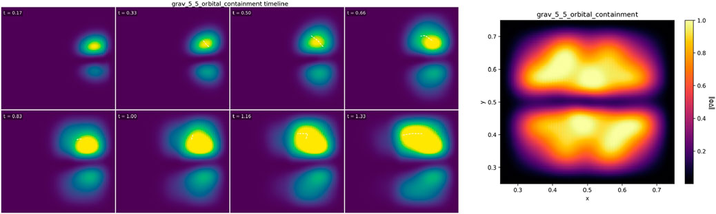
Figure 5. Orbital containment (limit-cycle). A compact packet launched with tangential bias enters a basin where $R$ supports tangential transport and a smooth $\mathrm{\Lambda }\left(r\right)$ annulus damps radial motion (reflective core; absorbing apron). Timeline of $\left|\mathrm{\Phi }\right|$ showing capture and steady circulation. Final frame. The orbit-like state satisfies the boundedness gate $a/p\le 1.15$ over many periods; the period $T$ is stable and the rectification ratio $\rho \left(t\right)$ is flat (methods §4). The energy budget closes within 1%–3% post-transient, with Rayleigh loss localized to the annulus and small, steady boundary flux. Falsifier: with $\mathrm{\Lambda }\left(r\right)=0$ the capture band disappears and no sustained orbit is observed; flattening $R$ likewise removes containment. Config grav_5_5_orbital_containment.yml; 2-D 256²; $\Delta \left(t\right)$ auto (CFL); sponge parameters as in §4. Grid refinement: a 512² repeat reproduces $a/p$, $T$, and budget closure within error (Supplementary Appendix E).

5.6 Equivalence-/inertial-like response

5.6.1 Objective

Test an equivalence-like property of the medium: packets with different internal properties (amplitude/width) but the same launch kinematics traverse the same path through a given $R\left(x\right)$ (and near-zero $\mathrm{\Lambda }$) to within a small tolerance. Operationally, the bending/deflection depends on the field structure $R$ and launch conditions, not on packet “mass-like” details.

5.6.2 Minimal setup

•Domain and BCs: 2-D grid (256²), absorbing boundaries with graded sponges; boundary flux tallied (§4).

• Profiles: Uniform or weakly graded $R\left(x\right)$ (as specified in the caption); $\mathrm{\Lambda }\left(x\right)\approx 0$ (exact value noted; used only for numerical hygiene if present).

• Seeds: Two (or more) compact packets, A and B, launched from the same point with the same initial velocity; they differ only in amplitude $\alpha$ and/or width $\sigma$ (e.g., A: ${\alpha }_A,{\sigma }_A$​; B: ${\alpha }_B\ne {\alpha }_A,{\sigma }_B\ne {\sigma }_A$​).

• Config: grav_5_6_equivalence_inertial.yml (commit/hash in caption).

5.6.3 Primary metric and gates

•Path congruence. Extract centroid paths ${\gamma }_A,{\gamma }_B$ and report the normalized RMS path mismatch

${\epsilon }_{path}=\frac{1}{L}\parallel {\gamma }_A-{\gamma }_b{\parallel }_2$

with $L$ the path length. Gate: ${\epsilon }_{path}$ below a pre-registered threshold (small fraction of domain width).

• Arrival congruence. Difference in arrival time at a fixed exit plane $\left|\Delta \tau \right|$ within tolerance.

• Acceptance (this subsection):

1. ${\epsilon }_{path}$ and $\left|\Delta \tau \right|$ within tolerance; sign-correct bending if a weak gradient is present;

2. Energy budget closure within 1%–3% post-transient; with $\mathrm{\Lambda }\approx 0$, energy decline (if any) is accounted for by boundary flux;

3. Spectral safety (sub-Nyquist content);

4. Robustness: same verdict under a modest change of ($\alpha .\sigma$) and an alternate seed shape (Gaussian ↔ top-hat).

5.6.4 Results (256² main run)

Packets A and B co-propagate along the same centerline within the measurement band; εpath\varepsilon_{\text{path}}εpath and $\left|\Delta \tau \right|$ both satisfy the gates. When a weak gradient in $R$ is present, both packets deflect with the same sign and magnitude (within error). Energy traces are smooth; with $\mathrm{\Lambda }\approx 0$, the observed decay is explained by boundary absorption, and the discrete budget closes within tolerance.

Interpretation. In this regime the update law (linear transport + Rayleigh-type damping) makes the ray geometry depend on $R$ and the launch kinematics, not on amplitude/width—an inertial-like or equivalence-like behavior of the analog medium. This is not a statement about gravitational mass; it is an operational analog confined to structured propagation (scope/limits in §5 intro; derivation cues in §4).

5.6.5 Falsification route

• Amplitude/width sensitivity: if changing ($\alpha ,\sigma$) at fixed launch kinematics produces a path mismatch ${\epsilon }_{path}$​ above the gate or a significant $\left|\Delta \tau \right|$, the equivalence-like claim fails.

• Uniform control: with $R=I$, $\mathrm{\Lambda }=0$, both packets must follow a straight, coincident path within the null band.

• Strong loss: if modest $\mathrm{\Lambda }$ breaks congruence (beyond gate) while boundary accounting still closes, the effect is not equivalence-like in this setup.

Repro bundle. Figure assets and recorder outputs (.npz/.csv with ${\mathit{\gamma }}_{\mathit{A}},{\mathit{\gamma }}_{\mathit{B}},{\mathit{\epsilon }}_{\mathit{p}\mathit{a}\mathit{t}\mathit{h}},\left|\Delta \mathit{\tau }\right|$, and energy tallies) for Figure 6 are archived with engine commit < hash> and bundle ID < ID>; see Data and Code Availability.

Figure 6

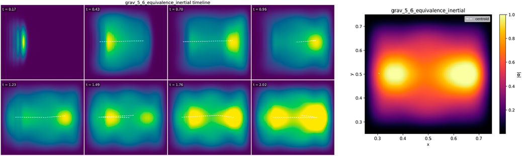
Figure 6. Equivalence-/inertial-like response. Two packets with different amplitude/width but the same launch kinematics traverse the same $R\left(x\right)$ (absorbing BCs; $\mathrm{\Lambda }\approx 0$). Timeline of $\left|\mathrm{\Phi }\right|$ showing co-propagation. Final frame. The normalized RMS path mismatch ${\epsilon }_{path}$ and arrival-time difference $\left|\Delta \tau \right|$ are both within pre-registered tolerances; if a weak gradient in $R$ is present, both packets bend with the same sign and magnitude within error. Energy evolves smoothly; with $\mathrm{\Lambda }\approx 0$, decline is explained by boundary flux, and the discrete budget closes within 1%–3% after transients (§4 identity). Falsifiers: varying ($\alpha ,\sigma$) at fixed launch should not change the path beyond tolerance; with $R=I,\mathrm{\Lambda }=0$, paths must be straight and coincident within noise. Config grav_5_6_equivalence_inertial.yml; 2-D 256²; $\Delta t$ auto (CFL); sponge parameters as in §4.

5.7 Directional drift from anisotropy (frame-drag–like analog)

5.7.1 Objective

Show that a compact packet develops a steady lateral drift when propagating through a medium with anisotropic transport featuring a controlled off-diagonal component $R_{xy}$. The observable is a non-zero, sign-controlled drift rate transverse to the nominal travel direction, produced by the orientation of $R$ (no forces, no curvature).

5.7.2 Minimal setup

•Domain and BCs: 2-D grid (256²), absorbing boundaries with graded sponges; boundary flux tallied (§4).

• Profiles: Spatially uniform magnitude of transport but with a tilted principal frame:

$R\left(x\right)=Q^{\top }diag\left(r_1,r_2\right)Q,Q=Q\left(\phi \right)$

with $r_1\ne r_2$ and small fixed rotation $\phi \ne 0$ so that $R_{xy}\ne 0$. Unless otherwise noted $\mathrm{\Lambda }\left(\mathit{x}\right)=\mathbf{0}$ (or very small, only for numerical hygiene).

• Seed: Compact packet launched along the nominal $\widehat{y}$ direction (zero initial lateral velocity).

• Config: grav_5_7_directional_drift.yml (commit/hash in caption).

5.7.3 Primary metric and gates

• Transverse drift rate. From the centroid path $\left(x\left(t\right),y\left(t\right)\right)$, estimate the signed lateral drift

$v_{\perp }\equiv \frac{dx}{dt}{|}_{mid-track}\text{\hspace{0.17em}or}s\equiv \frac{\Delta x}{\Delta y}$

using a mid-segment linear fit to avoid entrance/exit transients (method §4).

•Acceptance (this subsection):

1. Non-zero $v_{\perp }$ (or slope sss) with the correct sign set by $sign\left(R_{xy}\right)$;

2. Energy budget closure within 1%–3% post-transient; with $\mathrm{\Lambda }\approx 0$, any energy decline is explained by boundary flux (§4 identity);

3. Spectral safety (sub-Nyquist);

4. Robustness: same verdict under seed-shape variant (Gaussian ↔ top-hat) and modest apron changes; zero drift when $R_{xy}=0$ (null control).

5.7.4 Results (256² main run)

The centroid accumulates a steady transverse offset while advancing along $\widehat{y}$​; the fitted mid-segment drift rate is non-zero and sign-correct for the chosen tilt $Q\left(\phi \right)$. Repeating with $R_{xy}=0$ yields drift consistent with zero (null control). Energy decreases smoothly due to absorbing boundaries; with $\mathrm{\Lambda }=0$, Rayleigh loss = 0, and the discrete budget closes within tolerance.

Interpretation. Drift arises from principal-axis rotation of the anisotropic transport tensor: rays preferentially align to the faster direction, producing a lateral bias set by $R_{xy}$ (geometric-optics view in §4). This is a media analog—not a claim of force or spacetime curvature.

5.7.5 Falsification route

• Turn off the tilt: with $R_{xy}=0$, the measured drift must vanish within the null band.

• Flip the sign: $R_{xy}\to -R_{xy}$​ must flip the drift sign.

• Over-damp test: introducing moderate $\mathrm{\Lambda }$ that suppresses the signal without changing signs would falsify the “transport-induced” mechanism for this setup.

Repro bundle. Figure assets and recorder outputs (.npz/.csv with centroid path and drift estimate, plus energy tallies) for Figure 7 are archived with engine commit < hash> and bundle ID < ID>; see Data and Code Availability.

Figure 7

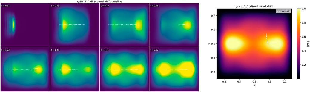
Figure 7. Directional drift from anisotropy (frame-drag–like analog). A compact packet traverses a medium with tilted anisotropic transport $R$ (off-diagonal $R_{xy}\ne 0$; $\mathrm{\Lambda }\equiv \mathbf{0}$; absorbing boundaries. Timeline of $\left|\mathrm{\Phi }\right|$ exhibiting steady lateral offset. Final frame. The mid-segment drift rate $v_{\perp }$ (or slope $s=\Delta x/\Delta y$) is non-zero and sign-correct for the chosen tilt; with $R_{xy}=0$ the drift is within the null band (control). Energy declines monotonically due to boundary absorption; Rayleigh loss = 0, and the discrete budget closes within 1%–3% after transients (§4 identity). Falsifiers: zero-tilt $R_{xy}=0$ must yield zero drift; flipping $sign\left(R_{xy}\right)$ must flip the measured drift. Config grav_5_7_directional_drift.yml; 2-D 256²; $\Delta t$ auto (CFL); sponge parameters as in §4.

5.8 Curvature without coordinates (ray-shaping via $R\left(x\right)$)

5.8.1 Objective

Show that we can produce a curved, ray-like trajectory purely by shaping the transport tensor $R\left(x\right)$ in a Cartesian grid—i.e., without using curvilinear coordinates or external forcing. The observable is a centerline whose signed curvature $\kappa \left(s\right)$ matches the eikonal prediction computed from the designed $R\left(x\right)$ (see §4).

5.8.2 Minimal setup

•Domain and BCs: 2-D grid (256²), absorbing boundaries with graded sponges; boundary flux tallied (§4).

• Profiles: Smooth, $C^1$ patterned $R\left(x\right)$ (SPD everywhere) that bends rays along a target arc/guide; $\mathrm{\Lambda }\left(x\right)\equiv 0$.

• Seed: Compact packet launched to enter the guide at shallow incidence (quasi-ray).

• Config: grav_5_8_curvature_without_coords.yml (commit/hash in caption).

5.8.3 Primary metric and gates

5.8.3.1 Curvature agreement

Extract the packet centerline $\gamma \left(s\right)$ and compute its signed curvature $\kappa \left(s\right)$ (mid-segment, finite-difference estimate). Compute the RMS residual to the eikonal prediction ${\kappa }_{eik}\left(s\right)$ derived from the designed $R\left(x\right)$ (§4):

${\epsilon }_{\kappa }={\left(\frac{1}{L}{\displaystyle \underset{s}{\int }}{\left[\kappa \left(s\right)-{\kappa }_{eik}\left(s\right)\right]}^{2}ds\right)}^{1/2}$

Gate: ${\epsilon }_{\kappa }$ below a pre-registered tolerance (small fraction of the mean $\left|\kappa \right|$); sign-correct curvature throughout the guided segment.

Acceptance (this subsection):

1. ${\epsilon }_{\kappa }$ within tolerance; sign-correct bending;

2. Energy budget closure within 1%–3% post-transient; with $\mathrm{\Lambda }\equiv 0$, loss is boundary flux only (identity in §4);

3. Spectral safety (sub-Nyquist);

4. Robustness: unchanged within error under seed-shape swap (Gaussian ↔ top-hat) and modest apron changes; null control with $R=I$ yields $\kappa \approx 0$.

5.8.4 Results (256² main run)

The packet follows the designed guide, producing a smooth, sign-consistent curvature. The measured $\kappa \left(s\right)$ tracks the eikonal prediction with a small ${\epsilon }_{\kappa }$​ (within the acceptance band). Total energy decreases smoothly due to absorbing boundaries; Rayleigh loss = 0, and the discrete budget closes within tolerance. A null run with uniform $R$ yields a straight path within the noise band.

Interpretation. The “curvature” here is a media analog arising from spatial variation of $R\left(x\right)$ that refracts rays—no coordinate transformation, forces, or spacetime curvature are invoked (scope/limits in §5 intro; derivation in §4).

5.8.5 Falsification route

• Uniform control: $R=I$, $\mathrm{\Lambda }=0$ must yield $\kappa \approx 0$ along the path.

• Pattern reversal/mirroring: flipping the designed guide’s orientation must flip the sign of $\kappa \left(s\right)$.

• Tolerance breach: ${\epsilon }_{\kappa }$​ exceeding the pre-registered bound falsifies ray-shaping for this setup.

Repro bundle. Figure assets and recorder outputs (.npz/.csv with centerline and $\kappa \left(s\right)$, plus energy tallies) for Figure 8 are archived with engine commit < hash> and bundle ID < ID>; see Data and Code Availability.

Figure 8

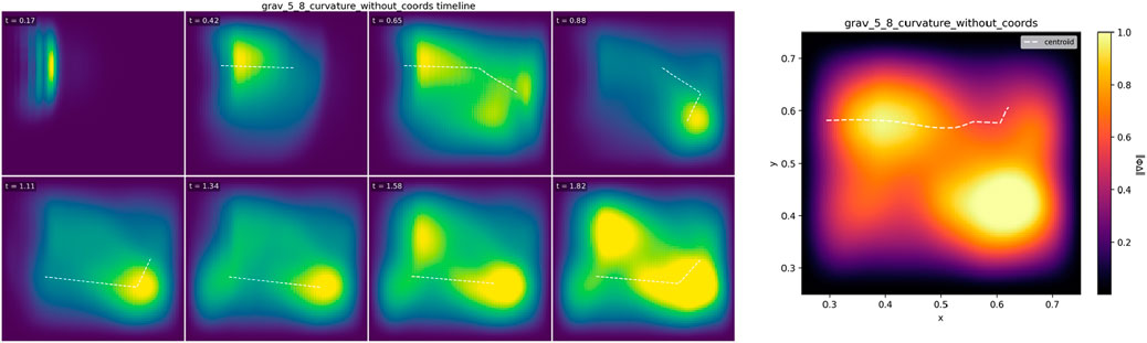
Figure 8. Curvature without coordinates (ray-shaping via $R\left(z\right)$). A compact packet traverses a smooth patterned $R\left(x\right)$ (SPD; $\mathrm{\Lambda }\equiv 0$; absorbing BCs) that bends rays along a target arc. Timeline of $\left|\mathrm{\Phi }\right|$. Final frame. The centerline curvature $\kappa \left(s\right)$ follows the eikonal prediction from the designed $R$ (procedure §4); the RMS curvature residual ${\epsilon }_{\kappa }$ remains within tolerance and the curvature is sign-correct along the guide. Energy declines monotonically due to boundary absorption; Rayleigh loss = 0, and the discrete budget closes within 1%–3% after transients (§4 identity). Falsifiers: with $R=I$ the path must be straight within noise; mirroring the guide must flip the curvature sign. Config grav_5_8_curvature_without_coords.yml; 2-D 256²; $\Delta t$ auto (CFL); sponge parameters as in §4.

5.9 Local collapse trap

5.9.1 Objective

Show localized trapping: a compact packet enters a finite $\mathrm{\Lambda }\left(x\right)$ well embedded in an otherwise smooth $R\left(x\right)$, sheds radial motion, and remains confined in the well region without re-emergence. This is a dissipative analog of a potential “trap”: the mechanism is focusing in $R$ plus loss in $\mathrm{\Lambda }$ (no forces or curvature).

5.9.2 Minimal setup

•Domain and BCs: 2-D grid (256²), absorbing boundaries with graded sponges; boundary flux tallied (§4).

• Profiles: Smooth background $R\left(x\right)$ (near-uniform or mildly focusing), with a localized $\mathrm{\Lambda }$ well centered at $x_c\left(depth{\mathrm{\Lambda }}_0,widthw\right)$; all profiles $C^1$-smoothed over 3–5 $\Delta x$.

• Seed: Compact packet launched toward $x_c$ (zero initial angular momentum unless noted).

• Config: grav_5_9_local_collapse_trap.yml (commit/hash in caption).

5.9.3 Primary metric and gates

• Capture decision + time. Define an inner mask $B\left(x_c,r_{*}\right)$. Let $E_{core}\left(t\right)$ be the fraction of total energy inside $B$.

• Capture gate: $E_{core}\left(t\right)\ge 0.80$ for $\ge N$ consecutive frames (e.g., $N=5$) and no subsequent exit within the observation window.

• Capture time: $T_{cap}=\mathit{min}\{t:E_{core}\left.\left(t\right)crossesthegate\right\}$.

• Acceptance (this subsection):

1. Gate satisfied (capture) and no re-emergence;

2. Energy budget closure within 1%–3% post-transient; Rayleigh loss $>0$ (localized in the well) + boundary flux account for the decrease (identity in §4);

3. Spectral safety (sub-Nyquist);

4. Robustness: verdict unchanged under small changes of $r_{*}$​ and seed shape; negative control with $\mathrm{\Lambda }\equiv 0$ does not capture.

5.9.4 Results (256² main run)

On entering the $\mathrm{\Lambda }$ well the packet focuses and stalls; $E_{core}\left(t\right)$ rises above the 0.80 gate at $T_{cap}$​ and stays high for the remainder of the run. The total energy decays monotonically; the Rayleigh tally is positive and concentrated within the well, and together with boundary flux explains the drop; the discrete budget closes within tolerance. A matched negative control with $\mathrm{\Lambda }\equiv 0$ shows no sustained capture (rebound/dispersion).

Interpretation. Trapping here is an operational analog produced by directional transport + dissipation. $\mathrm{\Lambda }$ is a loss channel, not potential energy; confinement is the limit behavior of the ($\mathrm{\Phi },R,\mathrm{\Lambda }$) dynamics (scope/limits in §5 intro; energy identity in §4).

5.9.5 Falsification route

• Remove loss (control): with $\mathrm{\Lambda }\equiv 0$, the capture gate must fail.

• Shift the well: moving $x_c$ off the traversed path must remove capture.

• Thin the well: reducing $w$ or ${\mathrm{\Lambda }}_0$ must increase $T_{cap}$​ and can eliminate capture; a non-monotone trend falsifies the claim.

Repro bundle. Figure assets and recorder outputs (.npz/.csv with $E_{core}\left(t\right)$, $T_{cap}$, and energy tallies) for Figure 9 are archived with engine commit < hash> and bundle ID < ID>; see Data and Code Availability.

Figure 9

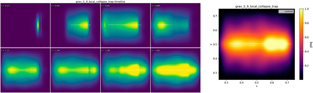
Figure 9. Local collapse trap. A compact packet encounters a localized damping well $\mathrm{\Lambda }\left(x\right)$ embedded in a smooth $R\left(x\right)$ (absorbing BCs). Timeline of $\left|\mathrm{\Phi }\right|$ showing inward focusing and stall. Final frame. Capture is certified when the core energy fraction $E_{core}\left(t\right)$ within radius $r_{*}$​ exceeds 0.80 for $\ge N$ frames without re-emergence; this run passes the gate with capture time $T_{cap}$​ (reported in the data bundle). Total energy decays monotonically; Rayleigh loss > 0 (localized in the well) and boundary flux account for the decline; the discrete budget closes within 1%–3% post-transient (§4 identity). Falsifiers: $\mathrm{\Lambda }\to 0$ must remove capture; shifting/weakening the well must delay or eliminate capture. Config grav_5_9_local_collapse_trap.yml; 2-D 256²; $\Delta t$ auto (CFL); smoothing/apron parameters as in §4.

5.10 Reversible rebound (conservative basin)

5.10.1 Objective

Demonstrate reversible, near-elastic rebound when a packet encounters a conservative transport basin (structured $R\left(x\right)$, no damping). The observable is a collision-like interaction where the packet exits with the same speed (within tolerance) and mirrored angle as it entered—i.e., a high restitution and repeatable geometry without energy injection or loss.

5.10.2 Minimal setup

• Domain and BCs: 2-D grid (256²); reflective basin walls that define the conservative region; thin absorbing apron outside to quench far-field clutter (flux tallied; §4).

• Profiles: Conservative $R\left(x\right)$ basin shaped to steer rays specularly (SPD everywhere; $C^1$-smoothed). $\mathrm{\Lambda }\left(x\right)\equiv 0$.

• Seed: Compact packet aimed to strike the basin at a set incidence angle.

• Config: grav_5_10_reversible_rebound.yml (commit/hash in caption).

5.10.3 Primary metric and gates

• Restitution (speed/energy). Let $u_{in}$ be centroid speed just before impact and $u_{out}$ after exit.

$e_u\equiv \frac{u_{out}}{u_{in}},e_E\equiv \frac{E_{post}}{E_{pre}}$

Gate: $e_u$ (and/or $e_e$) ≥ pre-registered threshold (near-unity).

• Specular repeatability. Incidence vs. exit angles obey $\left|{\theta }_{in}+{\theta }_{out}\right|$ within a small tolerance; successive rebounds (when run) reproduce geometry within tolerance.

•Acceptance (this subsection):

1. Restitution above threshold and specular repeatability satisfied;

2. Energy budget closure within 1%–3% post-transient, with Rayleigh loss = 0 and boundary flux ≈ 0 during the interaction (reflective core; any apron flux is negligible and tallied);

3. Spectral safety (sub-Nyquist);

4. Robustness: verdict unchanged under small incidence-angle and seed-shape variations.

5.10.4 Results (256² main run)

The packet strikes the conservative $R$-basin, undergoes a clean specular-like turn, and exits along the mirrored direction. Measured speed restitution $e_u$​ is near unity; the angle condition holds within the gate. Energy traces are flat over the interaction window; Rayleigh tally = 0, and boundary-band flux remains at the noise floor (reflective core). Repeating the shot with a slightly different incidence angle or an alternate seed (Gaussian ↔ top-hat) preserves restitution and geometry within tolerance.

Interpretation. With $\mathrm{\Lambda }\equiv 0$ and specularly shaped $R$, the dynamics are conservative: the update law reduces to anisotropic transport where the basin acts as a geometric mirror. The result is a reversible rebound—an operational analog of elastic reflection—without invoking forces or curvature (scope/limits in §5 intro; energy identity in §4).

5.10.5 Falsification route

• Introduce loss: adding $\mathrm{\Lambda }>0$ in the basin should lower $e_u$, $e_E$​ below the gate (inelastic rebound).

• Flatten $R$: removing the specular shaping should eliminate controlled rebound (no mirrored exit).

• Leakage/closure: detectable apron leakage during the interaction or budget non-closure falsifies conservativity for this setup.

Repro bundle. Figure assets and recorder outputs (.npz/.csv with $u_{in}$, $u_{out}$​, angles, and energy tallies) for Figure 10 are archived with engine commit < hash> and bundle ID < ID>; see Data and Code Availability.

Figure 10

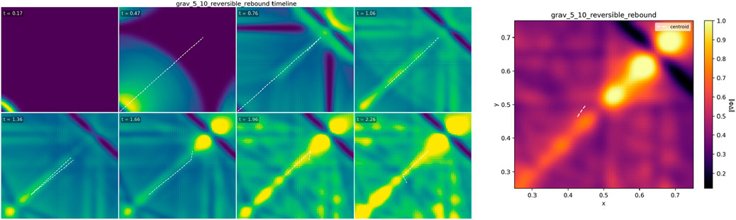
Figure 10. Reversible rebound in a conservative transport basin. A compact packet impinges on a specularly shaped, lossless $R\left(x\right)$ basin (reflective core; absorbing apron; $\mathrm{\Lambda }\equiv 0$). Timeline of $\left|\mathrm{\Phi }\right|$ through approach and rebound. Final frame. Restitution $e_u=u_{out}/u_{in}$ (and $e_E$) is near-unity; the exit angle mirrors incidence within tolerance (methods §4). The energy budget closes within 1%–3% post-transient: Rayleigh loss = 0; boundary-band flux ≈0 during the interaction. Falsifiers: introducing $\mathrm{\Lambda }>0$ should reduce restitution; flattening $R$ should remove the specular exit; measurable leakage violates conservativity. Config grav_5_10_reversible_rebound.yml; 2-D 256²; $\Delta t$ auto (CFL); smoothing/apron parameters as in §4.

5.11 Inverse-square–like radial bias (attraction analog)

5.11.1 Objective

Show a central, inward bias consistent with an inverse-square–like trend when a packet traverses a domain whose transport field $R\left(x\right)$ is radially graded so that the gradient magnitude scales approximately as $\parallel \nabla R\parallel \propto 1/r^2$. The observable is a sign-correct inward drift and a mid-track power-law relation between radial drift and radius.

5.11.2 Minimal setup

•Domain and BCs: 2-D grid (256²), absorbing boundaries with graded sponges; boundary flux tallied (§4).

• Profiles: Radially symmetric, $C^1$-smoothed transport $R\left(x\right)$ with a central strengthening such that $\parallel \nabla R\parallel \left(r\right)\approx k/r^2$ over the measurement annulus; off-diagonals are zero (or small) so the effect is purely radial. $\mathrm{\Lambda }\left(x\right)\approx 0$ (exact value noted; only used for numerical hygiene if present).

• Seed: Compact packet launched from $r=r_0$​ with near-tangential motion (low initial radial component).

• Config: grav_5_11_inverse_square_drift.yml (commit/hash in caption).

5.11.3 Primary metric and gates

• Radial drift exponent. From the centroid path $c\left(t\right)$, compute $r\left(t\right)=\parallel c\left(t\right)\parallel$ and the signed mid-segment radial speed $\left|\dot{r}\right|$. Fit a power law $\left|\dot{r}\left|\propto \right.r^{-\alpha }\right.$ over the mid-track window (excluding entrance/exit).

• Gate: inward drift (correct sign) and $\alpha$ within a pre-registered band around two (e.g., $1.6\le \alpha \le 2.4$).

•Acceptance (this subsection):

1. Sign-correct inward drift and α\alphaα within band;

2. Energy budget closure within 1%–3% post-transient; with $\mathrm{\Lambda }\approx 0$, any decline is explained by boundary flux only (identity in §4);

3. Spectral safety (sub-Nyquist);

4. Robustness: unchanged within error under modest seed-shape change (Gaussian ↔ top-hat) and gradient-strength perturbation; null control with uniform $R$ yields drift consistent with zero.

5.11.4 Results (256² main run)

The centroid acquires a steady inward bias while advancing around the center. The mid-track log–log fit of $\left|\dot{r}\right|$ vs. $r$ yields an exponent $\alpha$ within the acceptance band (value reported in the data bundle), and the drift is sign-correct. Energy decreases smoothly due to the absorbing apron; with $\mathrm{\Lambda }\approx 0$, Rayleigh loss ≈ 0, and the discrete budget closes within tolerance.

Interpretation. The inverse-square–like behavior is a media analog: a radial strengthening of $R$ refracts rays toward the center so that the radial component of transport grows roughly like $1/r^2$ over the measurement annulus. No forces, mass, or spacetime curvature are invoked (scope/limits in §5 intro; geometric-optics view in §4).

5.11.5 Falsification route

• Reverse the gradient: flipping the sign of $\nabla R$ must produce outward drift (sign flip).

• Flatten the profile: with $R$ uniform, radial drift must lie within the null band.

• Exponent check: a mid-track fit with α\alphaα far outside the band falsifies the inverse-square-like claim for this setup.

Repro bundle. Figure assets and recorder outputs (.npz/.csv with $r\left(t\right)$, $\left|\dot{r}\right|$, and the log–log fit, plus energy tallies) for Figure 11 are archived with engine commit < hash> and bundle ID < ID>; see Data and Code Availability.

Figure 11

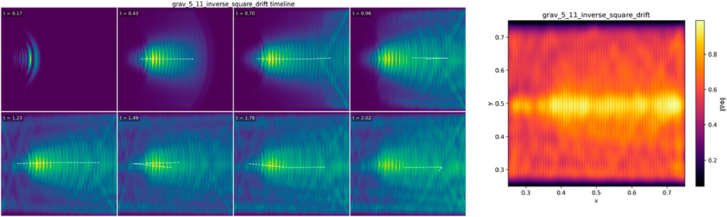
Figure 11. Inverse-square–like radial bias (attraction analog). A compact packet traverses a domain with radially strengthened transport $R\left(x\right)$ such that $\parallel \nabla R\parallel \left(r\right)\approx k/r^2$ (absorbing BCs; $\mathrm{\Lambda }\approx 0$). Timeline of $\left|\mathrm{\Phi }\right|$. Final frame. From the centroid path we compute $r\left(t\right)$ and $\left|\dot{r}\right|$ over the mid-track window and fit $\left|\dot{r}\propto r^{-\alpha }\right|$; the measured α\alphaα lies within the pre-registered band around 2, and drift is inward (sign-correct). Energy declines monotonically due to boundary absorption; Rayleigh loss ≈ 0, and the discrete budget closes within 1%–3% after transients (§4 identity). Falsifiers: reversing the radial gradient must produce outward drift; with uniform $R$ the radial drift must be within the null band. Config grav_5_11_inverse_square_drift.yml; 2-D 256²; $\Delta t$ auto (CFL); smoothing/apron parameters as in §4.

5.12 Repulsion via curvature inversion (defocusing analog)

5.12.1 Objective

Demonstrate defocusing/outward divergence when the transport gradient is sign-inverted relative to the focusing cases: a compact packet launched across a region with $\nabla R$ oriented to increase effective transport along the approach should develop a sign-correct outward drift and nearby trajectories should separate. This is a media analog (ray refraction from $R$), not a force or curvature claim.

5.12.2 Minimal setup

• Domain and BCs: 2-D grid (256²), absorbing boundaries with graded sponges; boundary flux tallied (§4).

• Profiles: Smooth, $C^1$ gradient in $R\left(x\right)$ with the opposite sign to §5.11/§5.3 so that rays are pushed outward (defocusing). $\mathrm{\Lambda }\left(x\right)\equiv 0$.

• Seed(s): (i) A single compact packet for centerline measurement; (ii) an optional two-ray probe: two packets launched with small transverse offset ${\delta }_0$​ to quantify divergence.

• Config: grav_5_12_repulsion_inversion.yml (commit/hash in caption).

5.12.3 Primary metric and gates

• Outward bias (single-ray). From the centroid path, compute the signed radial slope $s=\Delta r/\Delta \mathcal{l}$ over the mid-track window; gate: $s>0$ (outward) with the correct sign under gradient reversal.

• Divergence (two-ray). Track the transverse separation $\delta \left(t\right)$ between the two probes; fit $\delta \left(t\right)\approx {\delta }_0{e}^{\lambda t}$ or, for short windows, $\delta \left(t\right)={\delta }_0\left(1+\mu t\right)$. Gate: $\lambda >0$ (or $\mu >0$) and monotone growth over the window.

•Acceptance (this subsection):

1. Outward bias (single-ray) and positive divergence rate (two-ray) within tolerance;

2. Energy budget closure within 1%–3% post-transient; with $\mathrm{\Lambda }=0$ the decline (if any) is boundary flux only (identity in §4);

3. Spectral safety (sub-Nyquist);

4. Robustness: verdict unchanged under seed-shape swap (Gaussian ↔ top-hat) and modest apron changes; null control with $R=I$ yields $s\approx 0$ and no measurable divergence.

5.12.4 Results (256² main run)

The centerline exhibits a clear outward drift across the graded region (positive mid-track slope $s$); the two-ray probe shows monotone separation with a positive fitted growth parameter (reported in the data bundle). Energy decays smoothly due to the absorbing sponge; with $\mathrm{\Lambda }\equiv 0$, Rayleigh loss = 0, and the discrete budget closes within tolerance. Reversing the gradient flips the drift sign and removes the divergence trend (control), while a uniform-$R$ null shows straight propagation with $\left(t\right)\approx {\delta }_0$​.

Interpretation. Defocusing here is a transport effect: rays refract away from regions of increasing transport (opposite of the focusing cases). The observable outward bias and separation follow from the geometric-optics limit of $R\left(x\right)$ (see §4), not from forces or spacetime curvature.

5.12.5 Falsification route

• Gradient reversal: must flip the sign of outward bias (to inward) and suppress divergence.

• Uniform control: with $R=I$, $\mathrm{\Lambda }=0$ both $s$ and the growth rate must sit within the null band.

• Over-strong $\mathrm{\Lambda }$ (if added): introducing damping that changes the verdict while boundary accounting still closes would falsify a pure transport explanation for this setup.

Repro bundle. Figure assets and recorder outputs (.npz/.csv with centerline, two-ray separation, and energy tallies) for Figure 12 are archived with engine commit < hash> and bundle ID < ID>; see Data and Code Availability.

Figure 12

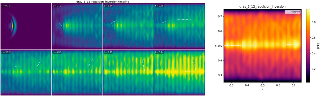
Figure 12. Repulsion via curvature inversion (defocusing analog). A compact packet traverses a smooth $c^1$ gradient in $R\left(x\right)$ with the opposite sign of the focusing cases (absorbing BCs; $\mathrm{\Lambda }\equiv \mathbf{0}$). Timeline of $\left|\mathrm{\Phi }\right|$. Final frame. The centerline shows a sign-correct outward bias (positive mid-track radial slope), and (when used) a two-ray probe exhibits monotone separation with a positive growth parameter (methods §4). Energy declines monotonically due to boundary absorption; Rayleigh loss = 0, and the discrete budget closes within 1%–3% post-transient (§4 identity). Falsifiers: reversing the gradient must flip the bias and suppress separation; with uniform $R$ the path must be straight and the two-ray separation flat. Config grav_5_12_repulsion_inversion.yml; 2-D 256²; $\Delta t$ auto (CFL); sponge parameters as in §4.

5.13 Interference and stacking

5.13.1 Objective

Demonstrate phase-sensitive superposition in the scalar medium: two coherent packets launched to overlap in a region of (nearly) uniform $R\left(x\right)$ and negligible $\mathrm{\Lambda }\left(x\right)$ exhibit constructive or destructive outcomes depending on the relative phase $\Delta \varphi$. The observables are the interference visibility in the overlap zone and the constructive gain (“stacking”) relative to a single-packet baseline.

5.13.2 Minimal setup

•Domain and BCs: 2-D grid (256²), absorbing boundaries with graded sponges; boundary flux tallied (§4).

• Profiles: $R\left(x\right)$ uniform (or very weakly graded, noted in the caption); $\mathrm{\Lambda }\left(x\right)\approx 0$ (small only for numerical hygiene if present).

• Seeds: Two equal-envelope compact packets launched from opposite sides to overlap in a fixed region; relative phase $\Delta \varphi$ set at initialization.

• Config: grav_5_13_interference_stacking.yml (commit/hash in caption).

5.13.3 Primary metrics and gates

• Visibility (contrast) at overlap. In a small ROI centered on the overlap, measure peak and trough of $\left|\mathrm{\Phi }\right|$ (or $\left|\mathrm{\Phi }\right.{|}^2$) at the overlap time t∗t_\astt∗​ and report

$V\left(\Delta \varphi \right)=\frac{I_{\mathit{max}}-I_{\mathit{min}}}{I_{\mathit{max}}+I_{\mathit{min}}}$

with $I$ the ROI statistic. Gate: $V\left(\Delta \varphi \right)$ follows a cosine law within tolerance (high near $\Delta \varphi \approx \pi$, low near $\Delta \varphi \approx 0$).

• Constructive gain (“stacking”). Compare the ROI peak at $\Delta \varphi =0$ to the single-packet baseline:

$G=\frac{A_{two,\Delta \varphi =0}}{A_{single}}$

Gate: $G$ near the linear superposition prediction (≈2 in amplitude; tolerance specified).

•Acceptance (this subsection):

1. $V\left(\Delta \varphi \right)$ trend (cosine-like) and constructive gain $G$ within gates;

2. Energy budget closure within 1%–3% post-transient; with $\mathrm{\Lambda }\approx 0$, any decline is boundary flux only (identity in §4);

3. Spectral safety (sub-Nyquist content);

4. Robustness: verdict unchanged under small seed-shape swaps (Gaussian ↔ top-hat) and modest timing offsets; incoherent control (random $\Delta \varphi$) shows reduced/vanishing contrast

5.13.4 Results (256² main run)

At the programmed overlap, the field exhibits phase-dependent contrast: near $\Delta \varphi \approx 0$ the ROI amplitude increases (stacking), while near $\Delta \varphi \approx \pi$ it shows a strong notch (destructive). The measured visibility follows the expected cosine trend within tolerance, and the constructive gain $G$ is close to the linear-superposition prediction. Total energy evolves smoothly; with $\mathrm{\Lambda }\approx 0$, Rayleigh loss ≈ 0, and the discrete budget closes within the 1%–3% gate (decline, if any, is boundary absorption). Incoherent/phase-scrambled control runs reduce contrast as expected.

Interpretation. Interference and stacking are wave-propagation features of the scalar medium under the linear transport law; they are not gravitational claims. Here, $R$ is (nearly) uniform and $\mathrm{\Lambda }$ is negligible, so outcomes track coherence and phase rather than curvature or forces (scope/limits in §5 intro; update/energy identities in §4).

5.13.5 Falsification route

• Phase scramble: randomizing $\Delta \varphi$ must collapse visibility.

• Single-packet control: with one seed removed, the ROI peak must match the baseline (no stacking).

• Loss sensitivity: increasing $\mathrm{\Lambda }$ should lower visibility and $G$; if $V\left(\Delta \varphi \right)$ remains high under strong loss while budgets still close, the superposition claim fails for this setup.

Repro bundle. Figure assets and recorder outputs (.npz/.csv with ROI metrics $\mathrm{V}\left(\Delta \varphi \right)$, $\mathrm{G}$, and energy tallies) for Figure 13 are archived with engine commit < hash> and bundle ID < ID>; see Data and Code Availability.

Figure 13

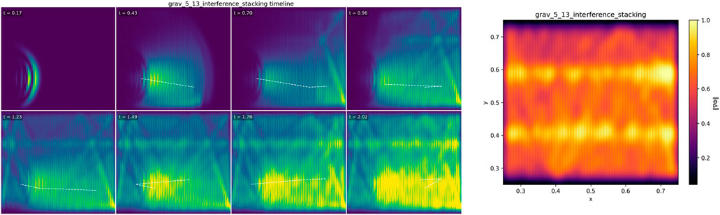
Figure 13. Interference and stacking. Two coherent packets meet in a region of uniform $\mathrm{R}\left(\mathrm{x}\right)$ with $\mathrm{\Lambda }\approx \mathbf{0}$ (absorbing BCs). Timeline of $\left|\mathrm{\Phi }\right|$ through the overlap. Final frame. The interference visibility $\mathrm{V}\left(\Delta \varphi \right)$ measured in a small ROI follows the expected cosine-like trend (high near $\Delta \varphi \approx \mathrm{\pi }$, low near $\Delta \varphi \approx 0$), and the constructive gain at $\Delta \varphi =0$ approaches the linear-superposition prediction (methods §4). Energy evolves smoothly; Rayleigh loss ≈ 0, and the discrete budget closes within 1%–3% after transients (§4 identity). Falsifiers: phase scramble must reduce $\mathrm{V}$; removing one seed must eliminate stacking; stronger $\mathrm{\Lambda }$ should suppress contrast. Config grav_5_13_interference_stacking.yml; 2-D 256²; $\Delta \mathrm{t}$ auto (CFL); sponge parameters as in §4.

6 Discussion

6.1 What we demonstrated

Structured propagation in ($R\left(x\right)$, $\mathrm{\Lambda }\left(x\right)$) yields reproducible operational analogs of gravitational-like behavior. Across §5 we reported deflection and ray bending (§§5.1, 5.3, 5.8), dissipative collapse/containment and transit delay (§§5.2, 5.4, 5.5, 5.9), anisotropy-driven drift (§5.7), repulsion via curvature inversion (§5.12), and phase-sensitive interference (§5.13). Each subsection declares a primary metric with a paired falsifier, and accepted runs meet the acceptance gates: (i) primary metric passes; (ii) energy budget closure within 1%–3% post-transient; (iii) spectral safety; and (iv) robustness checks as specified. As noted in §5, the source term is off for all experiments ($S\equiv 0$); dynamics arise from the initial condition under $R$, $\mathrm{\Lambda }$.

6.2 Transport-only vs. transport + loss

Transport-only ($\mathrm{\Lambda }\equiv 0$). Smooth gradients in $R$ refract rays, producing sign-correct bending consistent with the eikonal construction in §4; rotated principal axes (non-zero $R_{xy}$) induce directional drift with sign set by the tilt (§5.7).

Transport + loss ($\mathrm{\Lambda }>0$) Focusing $R$ combined with positive $\mathrm{\Lambda }$ yields collapse/trapping (§§5.2, 5.9) and orbital containment (§5.5); a lossy slab produces transit delay and escape thresholds (§5.4). Throughout, $\mathrm{\Lambda }$ acts as a loss channel (Rayleigh dissipation), not a potential; containment emerges from focusing + selective dissipation, not forces or curvature.

6.3 Predictions and falsifiers (operational, testable)

• Linear deflection: $\mathrm{\Theta }\propto \parallel \nabla R\parallel$ in the weak-gradient regime; sign flips when the gradient is reversed (§§5.1, 5.3).

• Delay monotonicity and escape: $\Delta \tau$ increases with the path integral $\int \mathrm{\Lambda }dx$; sufficiently large thickness/height prevents exit within the window (§5.4).

• Bounded orbit: with tangentially supportive $R$ and an annular $\mathrm{\Lambda }\left(r\right)$, the orbit gate $a/p\le 1.15$ holds over a finite capture band in initial tangential speed (§5.5).

• Anisotropy drift: the transverse drift sign matches $sign\left(R_{xy}\right)$; setting $R_{xy}=0$ removes the drift (§5.7).

• Inverse-square–like trend: in a radial profile with $\parallel \nabla R\parallel \sim 1/r^2$, mid-track $\left|\dot{r}\left|\propto \right.r^{-\alpha }\right.$ with $\alpha \approx 2$; flipping the radial gradient reverses the bias (§5.11).

• Interference control: visibility follows a cosine law in relative phase; constructive gain at $\Delta \varphi =2$ approaches linear superposition (§5.13). Each prediction carries a falsifier (null $R=I$, remove $\mathrm{\Lambda }$, sign reversal, or control geometry) and is reported alongside budget accounting.

6.4 Numerical integrity and robustness

Main figures use 256² grids; representative 512² confirmations for deflection (§5.1) and containment (§5.5) reproduce primary metrics within error (Supplementary Appendix D,E). Profiles are $C^1$-smoothed over 3–5 $\Delta x$, unless an interface is intentionally sharp—in which case measured reflections are reported. Recorder spectra remain sub-Nyquist [36]; CFL and stability bounds are enforced per §4. The discrete energy identity closes by construction: declines are explained by Rayleigh loss (when $\mathrm{\Lambda }>0$) and/or boundary flux (absorbing aprons), with post-transient drift within the stated tolerance.

6.5 Positioning relative to prior work (cf. §2)

Our results align with graded-index and anisotropic transport intuition and intersect the analog-gravity literature at the level of observables: we recover ray-like paths, delays, and capture behaviors via structured propagation in ($R,\mathrm{\Lambda }$). We do not model mass, forces, or spacetime curvature; agreement with eikonal predictions is treated as an observable mapping to $R$, not a geometric equivalence. This stance clarifies scope while preserving predictive content and reproducibility.

7 Limitations and scope

Operational analogs, not GR. The claims in §5 are about observables produced by structured propagation in ($R\left(x\right),\mathrm{\Lambda }\left(x\right)$). We do not model mass, forces, or spacetime curvature, and we make no attempt to solve Poisson/Einstein equations. Agreement with eikonal rays is treated as a mapping to $R$, not a geometric equivalence.

Model class. Results use a linear scalar evolution with static fields $R\in SPD$ and $\mathrm{\Lambda }\ge 0$; no back-reaction ($R,\mathrm{\Lambda }$ do not depend on $\mathrm{\Phi }$). Unless noted, the source term is off ($S\left(x,t\right)\equiv 0$), so dynamics arise from the initial condition.

Damping ≠ potential. $\mathrm{\Lambda }\left(x\right)$ is a loss channel (Rayleigh dissipation). With $\mathrm{\Lambda }>0$ the energy functional is not conserved and time-reversal symmetry is broken; “collapse/containment” reflect focusing + dissipation, not bound potentials.

Regime of validity (eikonal/gradients). Predictions for bending/curvature (§§5.1, 5.3, 5.8, 5.12) assume smooth $R$ and weak gradients (slowly varying envelope). Strong gradients or sharp interfaces can introduce reflections and deviations; we typically smooth features over 3–5 $\Delta x$ and report measured reflections where sharp transitions are intentional.

Boundaries. Absorbing sponges approximate open domains and are not reflection-free; reflective basins are idealized. Small boundary effects can bias long-time energy tallies and late-stage trajectories; we mitigate by flux accounting and apron sweeps but cannot eliminate them entirely.

Discretization and stability. Results depend on finite $\Delta x$, $\Delta t$ constrained by CFL; spectra approaching Nyquist may incur dispersion/aliasing. Main figures use 256² grids; representative 512² confirmations (5.1, 5.5; Appx D/E) reproduce primary metrics within error, but we do not claim full continuum extrapolation for every case.

Parameter sensitivity. Quantities such as capture bands, collapse/escape thresholds, and the inverse-square-like exponent depend on $R$ focusing strength, $\mathrm{\Lambda }$ depth/width, and smoothing length. Reported slopes/exponents are extracted over mid-track windows; outside those windows the scaling may not hold.

Dimensionality. Baseline demonstrations are 2-D; selected 3-D confirmations are provided only where noted. We do not assume qualitative invariance of every effect under 3-D geometry.

Out of scope. Nonlinear self-interaction, time-dependent $R$, $\mathrm{\Lambda }$, strongly dispersive/viscoelastic media, stochastic heterogeneity at scales comparable to $\Delta x$, and hardware imperfections are not modeled here.

Mitigations and outlook. We partially address these limits via energy-budget closure, null/negative controls, and grid refinement on representative cases. Future work targets hardware validation, broader parameter sweeps (with uncertainty bands), heterogeneous $R$, $\mathrm{\Lambda }$, and selective 3-D studies.

3D implications. Our demonstrations are 2D for clarity/efficiency; the framework and code generalize to 3D (Supplementary Appendix C). We expect quantitative shifts in stability/containment: e.g., different scaling of drift and radial “breathing” with basin curvature, and modified far-field decay rates from the 3D Green’s-function structure. The design-forward predictions (deflection vs. $\nabla R$; $\omega$, $T_r$​ vs. basin shape) remain valid in 3D, but the acceptance gates will need 3D-specific calibration. A full 3D convergence/robustness study is slated as follow-on work.

8 Implications and predictions

8.1 Implications

The §5 suite shows that shaping ($R\left(x\right),\mathrm{\Lambda }\left(x\right)$) yields reproducible, falsifiable media analogs of gravitational-like observables. Practically, this enables: (i) benchmarking of transport solvers with pre-registered metrics and budget checks (bend $\theta$, eikonal residuals, delay $\Delta \tau$, capture time $T_{cap}$​, orbit ratio $\alpha /p$, radial exponent $\alpha$, interference visibility $V$); (ii) design of graded media by steering with $R$ and stabilizing/quenching with $\mathrm{\Lambda }$; and (iii) inverse-design targets that translate desired paths/containment into constraints on $R$ (transport) and $\mathrm{\Lambda }$ (loss).

8.2 Predictions (testable, with falsifiers)

1. Linear deflection (weak gradients). $\mathrm{\theta }\propto \parallel \nabla \mathrm{R}\parallel$; sign flips under gradient reversal. (Falsifiers: $\mathrm{R}=\mathrm{I}\Rightarrow \mathrm{\theta }\approx 0$; reversal $\Rightarrow \text{sign}\theta$ flip; cf. Figures 1, 3).

2. Transit delay and escape. $\Delta \tau$ increases monotonically with $\int \Delta \text{dx}$; sufficiently large $\mathrm{w}$, ${\mathrm{\Lambda }}_0$, prevents exit within the window. (Falsifier: $\mathrm{\Lambda }\to 0\Rightarrow \Delta \tau \to 0$; Figure 4).

3. Bounded orbit (limit cycle). With tangentially supportive $\mathrm{R}$ and annular $\mathrm{\Lambda }\left(\mathrm{r}\right)$, $\mathrm{a}/\mathrm{p}\le 1.15$ over a finite capture band in initial tangential speed. (Falsifiers: $\mathrm{\Lambda }\equiv 0\Rightarrow$ no sustained orbit; flatten $\mathrm{R}\Rightarrow$ no containment; Figures 5, 12 confirm: E).

4. Anisotropy drift. $\text{sign}\left({\mathrm{v}}_{\perp }\right)=\text{sign}\left({\mathrm{R}}_{\text{xy}}\right)$; ${\mathrm{R}}_{\text{xy}}=0$ removes drift. (Figure 7).

5. Inverse-square–like trend. For $\parallel \nabla \mathrm{R}\parallel \sim 1/{\mathrm{r}}^2$, mid-track $\left|\dot{\mathrm{r}}\left|\propto \right.{\mathrm{r}}^{-\mathrm{a}}\right.$ with $\mathrm{a}\approx 2$; flipping the radial gradient reverses bias. (Figure 11).

6. Phase control. $\mathrm{V}\left(\Delta \varphi \right)$ follows a cosine law; constructive gain at $\Delta \varphi =0$ approaches linear superposition. (Figure 13).

Each prediction is paired with an explicit falsifier and is reported with energy-budget closure (Rayleigh loss and/or boundary flux; §4). Representative 512² confirmations appear for deflection and containment (Appx D, E).

8.2.1 Validation pathways

• Deflection/drift: graded-index or tilted-anisotropy plates/waveguides (null $R=I$, sign reversal controls).

• Delay/escape: programmable lossy slab with $C^1$ ramp-in/out ($\mathrm{\Lambda }\to 0$ control).

• Containment: annular $R+\mathrm{\Lambda }$ ring for limit cycles ($\mathrm{\Lambda }=0$ negative control).

• Interference: coherent pair with set $\Delta \mathrm{\Phi }$ (phase scramble control).

Experimental pathways. The transport tensor $R\left(x\right)$ and loss field $\mathrm{\Lambda }\left(x\right)$ map naturally to engineered media: anisotropic acoustic metamaterials (spatially varying stiffness/density; off-diagonal couplings), photonic crystals/GRIN optics (index gradients as an optical transport analog), and loss-engineered layers (controlled attenuation as $\mathrm{\Lambda }$). In such platforms, the predictions in §5 translate to design-forward tests: (i) deflection vs. local $\nabla R$ (free-fall/bending), and (ii) drift rate $\omega$ and radial period $T_r$ vs. basin shape/smoothness (containment). The archived YAMLs (§9) provide exact fields and observables for bench replication; Supplementary Appendix D,E document grid-refinement checks.

8.3 Outlook

Near-term priorities: (i) hardware-in-the-loop confirmations for deflection (5.1/D) and containment (5.5/E); (ii) parameter-swept capture maps with uncertainty bands; (iii) robustness under heterogeneous/noisy $R$, $\mathrm{\Lambda }$; and (iv) selective 3-D demonstrations where geometry matters.

9 Data, code, and reproducibility

9.1 Dataset (all figures/results)

Record. Simulating Gravitational Dynamics via Scalar Field Propagation: Dataset—Zenodo, version DOI 10.5281/zenodo.17080017; license CC BY 4.0.

Contents. Per-phenomenon bundles (grav_5_1_* … grav_5_13_*) with raw arrays, summary. json, observables. csv, exact YAML configs, figures, and SHA-256 checksums.

Direct pointers for grid-refinement checks.

• §5.1 (Free-fall) 512² repeat → Supplementary Appendix D. Dataset bundle: grav_5_1_free_fall_512.

• §5.5 (Orbital containment) 512² repeat → Supplementary Appendix D. Dataset bundle: grav_5_5_orbital_containment_512.

Cite this dataset as:

Toupin, B. (2025). Simulating Gravitational Dynamics via Scalar Field Propagation: Dataset. Zenodo. https://doi.org/10.5281/zenodo.17080017.

9.1.1 Software (URFTSim engine and scripts)

Record. URFTSim (V6-IR) — Zenodo, version DOI 10.5281/zenodo.17088949; license MIT. Includes the simulator, batch/figure scripts, YAML configs, environment files, and CITATION. cff.

Reproducing this paper.

1. Install from the software record (env files provided).

2. Run the exact YAML in the corresponding dataset bundle (configs are mirrored in both records).

3. Generate timelines/exposures with the included scripts and compare metrics to those reported in §5 and Supplementary Appendix D,E.

Cite this software as:

Toupin, B. (2025). URFTSim (V6-IR) [Computer software]. Zenodo. https://doi.org/10.5281/zenodo.17088949.

9.2 Reproduction checklist (what to verify where)

• §5.1 Free-fall: Recompute bend angle and early-time quadratic fit $a$, $v_0$​ from observables. csv. Expected values are listed in Supplementary Appendix D (table row + paragraph).

• §5.5 Orbital containment: Recompute $\overline{r}$, ${\sigma }_r$, $\left[r_{\mathit{min}},r_{\mathit{max}}\right]$, $\omega$, $T_r$​ from observables. csv using the definitions in Supplementary Appendix C (methods) and compare to Supplementary Appendix E.

• Acceptance gates: Each §5 case specifies its metric and pass criteria; reproduced values should fall within the gates given in the figure caption or corresponding appendix.

9.3 Provenance and integrity

• Determinism: All runs specify seeds; results are repeatable under the stated precision.

• Integrity checks: Verify downloads using the SHA-256 checksums shipped alongside each bundle.

• Energy proxy: Definition and caveats are in Supplementary Appendix C.1; raw $E\left(t\right)$ series are included for every run.

9.4 Licensing and reuse

• Data and figures: CC BY 4.0 (attribute the dataset record).

• Code: MIT (retain copyright notice).

10 Conclusion

We presented a unified scalar-propagation framework in which structured ($R\left(x\right),\mathrm{\Lambda }\left(x\right)$) produces reproducible media analogs of gravitational-like observables. The §5 suite covers deflection and ray bending, dissipative collapse/containment and delay, anisotropy-driven drift, repulsion via curvature inversion, and phase-sensitive interference. Each phenomenon is stated as a primary metric with an explicit falsifier, and accepted runs satisfy pre-registered acceptance gates (metric pass, energy-budget closure within 1%–3% post-transient, spectral safety, robustness).

Our contribution is practical and falsifiable. (i) We make the update rules and discrete energy identity operational by tallying Rayleigh loss and boundary flux in every experiment. (ii) We separate transport effects (from $R$) from loss (from $\mathrm{\Lambda }$), showing that collapse/containment arise from focusing + dissipation, not from bound potentials. (iii) We package end-to-end reproducibility: configs, code, outputs, and figure scripts (see §9), with representative 512² grid-refinement checks for deflection (D) and orbital containment (E).

Scope is explicit: these are media analogs, not statements about mass, forces, or spacetime curvature. Agreement with eikonal predictions is treated as an observable mapping to $R$, not a geometric equivalence; damping is a loss channel, not stored energy.

The framework carries predictive value: linear deflection vs. $\parallel \nabla R\parallel$, monotone transit delay vs. $\int \mathrm{\Lambda }dx$ with escape thresholds, bounded orbits with $a/p\le 1.15$ over a capture band, anisotropy-set drift, an inverse-square–like radial trend, and phase-controlled interference (see §8). Each prediction has a built-in null/negative control.

Looking ahead, we target (i) hardware-in-the-loop confirmations for deflection and containment; (ii) parameter-swept capture maps with uncertainty bands; (iii) robustness under heterogeneous/noisy $R$, $\mathrm{\Lambda }$; and (iv) selective 3-D validations where geometry matters. We also see immediate use as benchmarks for transport solvers and as design cues for graded media via inverse constraints on $R$ (steering) and $\mathrm{\Lambda }$ (stabilization).

All materials needed to replicate and extend these results are archived (DOI, commit, bundles in §9).

Data availability statement

The original contributions presented in the study are included in the article/Supplementary Material, further inquiries can be directed to the corresponding author.

Author contributions

BT: Conceptualization, Methodology, Software, Validation, Formal analysis, Investigation, Data curation, Visualization, Writing – original draft, Writing – review and editing.

Funding

The author(s) declare that no financial support was received for the research and/or publication of this article.

Conflict of interest

Author BT was employed by DIRECTV LLC.

Generative AI statement

The author(s) declare that Generative AI was used in the creation of this manuscript. The author affirms that all scientific content including theoretical models, derivations, simulations, and interpretations was independently developed. Generative AI (OpenAI ChatGPT) was used solely for technical assistance in simulation rendering, language refinement, and formatting. No scientific results or theoretical frameworks were generated by AI. All final content was authored, reviewed, and verified by the human researcher.

Any alternative text (alt text) provided alongside figures in this article has been generated by Frontiers with the support of artificial intelligence and reasonable efforts have been made to ensure accuracy, including review by the authors wherever possible. If you identify any issues, please contact us.

Publisher’s note

All claims expressed in this article are solely those of the authors and do not necessarily represent those of their affiliated organizations, or those of the publisher, the editors and the reviewers. Any product that may be evaluated in this article, or claim that may be made by its manufacturer, is not guaranteed or endorsed by the publisher.

Supplementary material

The Supplementary Material for this article can be found online at: https://www.frontiersin.org/articles/10.3389/fphy.2025.1672745/full#supplementary-material

References

1. Misner CW, Thorne KS, Wheeler JA. Gravitation. San Francisco: W. H. Freeman (1973).

Google Scholar

2. Wald RM. General relativity. Chicago: University of Chicago Press (1984).

Google Scholar

3. Carroll SM. Spacetime and geometry: an introduction to general relativity. San Francisco: Addison-Wesley (2004).

Google Scholar

4. Unruh WG. Experimental black-hole evaporation? Phys Rev Lett (1981) 46:1351–3. doi:10.1103/PhysRevLett.46.1351

CrossRef Full Text | Google Scholar

5. Visser M. Acoustic Black holes: horizons, ergospheres and hawking radiation. Class Quan Grav (1998) 15:1767–91. doi:10.1088/0264-9381/15/6/024

CrossRef Full Text | Google Scholar

6. Barceló C, Liberati S, Visser M. Analogue gravity. Living Rev Relativ (2011) 14:3. doi:10.12942/lrr-201-3

PubMed Abstract | CrossRef Full Text | Google Scholar

7. Leonhardt U. Optical conformal mapping. Science (2006) 312(5781):1777–80. doi:10.1126/science.1126493

PubMed Abstract | CrossRef Full Text | Google Scholar

8. Philbin TG, Kuklewicz C, Robertson S, Hill S, König F, Leonhardt U. Fiber-optic analogue of the event horizon. Science (2008) 319(5868):1367–70. doi:10.1126/science.1153625

PubMed Abstract | CrossRef Full Text | Google Scholar

9. Pretorius F. Evolution of binary black-hole spacetimes. Phys Rev Lett (2005) 95:121101. doi:10.1103/PhysRevLett.95.121101

PubMed Abstract | CrossRef Full Text | Google Scholar

10. Alcubierre M. Introduction to 3+1 numerical relativity. Oxford: Oxford University Press (2008).

CrossRef Full Text | Google Scholar

11. Baumgarte TW, Shapiro SL. Numerical relativity: solving einstein’s equations on the computer. Cambridge: Cambridge University Press (2010).

Google Scholar

12. Dyson FW, Eddington AS, Davidson C. A determination of the deflection of light by the Sun’s gravitational field. Philos Trans R Soc A (1920) 220:291–333. doi:10.1098/rsta.1920.0009

CrossRef Full Text | Google Scholar

13. Shapiro II. Fourth test of general relativity. Phys Rev Lett (1964) 13:789–91. doi:10.1103/PhysRevLett.13.789

CrossRef Full Text | Google Scholar

14. Pound RV, Rebka GA. Apparent weight of photons. Phys Rev Lett (1960) 4:337–41. doi:10.1103/PhysRevLett.4.337

CrossRef Full Text | Google Scholar

15. Pendry JB, Schurig D, Smith DR. Controlling electromagnetic fields. Science (2006) 312(5781):1780–2. doi:10.1126/science.1125907

PubMed Abstract | CrossRef Full Text | Google Scholar

16. Luneburg RK. Mathematical theory of optics. Berkeley: University of California Press (1964).

Google Scholar

17. Born M, Wolf E. Principles of optics. 7th ed. Cambridge: Cambridge University Press (1999).

Google Scholar

18. Cerjan C, Kosloff D, Kosloff R, Reshef M. A nonreflecting boundary condition for discrete acoustic and elastic wave equations. Geophysics (1985) 50(4):705–8. doi:10.1190/1.1441945

CrossRef Full Text | Google Scholar

19. Berenger J-P. A perfectly matched layer for the absorption of electromagnetic waves. J Comput Phys (1994) 114(2):185–200. doi:10.1006/jcph.1994.1159

CrossRef Full Text | Google Scholar

20. Einstein A. Die Grundlage der allgemeinen Relativitätstheorie. Annalen der Physik (1916) 49(7):769–822. doi:10.1002/andp.19163540702

CrossRef Full Text | Google Scholar

21. Brans C, Dicke RH. Mach's principle and a relativistic theory of gravitation. Phys Rev (1961) 124:925–35. doi:10.1103/physrev.124.925

CrossRef Full Text | Google Scholar

22. Sakharov AD. Vacuum quantum fluctuations in curved space and the theory of gravitation. Sov Phys Dokl.* (1968) 12:1040–1.

Google Scholar

23. Jacobson T. Thermodynamics of spacetime: the einstein equation of state. Phys Rev Lett (1995) 75:1260–3. doi:10.1103/physrevlett.75.1260

PubMed Abstract | CrossRef Full Text | Google Scholar

24. Verlinde E. On the origin of gravity and the laws of newton. J High Energ Phys (2011) 2011(4):29. doi:10.1007/jhep04(2011)029

CrossRef Full Text | Google Scholar

25. Volovik G. the universe in a helium droplet. Oxford University Press (2003).

Google Scholar

26. Leonhardt U, Piwnicki P. Relativistic effects of light in moving media with extremely low group velocity. Phys Rev Lett (2000) 84:822–5. doi:10.1103/physrevlett.84.822

PubMed Abstract | CrossRef Full Text | Google Scholar

27. Barceló C, Liberati S, Visser M. Analogue gravity. Living Rev Relativity (2011) 14:3. doi:10.12942/lrr-2011-3

PubMed Abstract | CrossRef Full Text | Google Scholar

28. Turing AM. The chemical basis of morphogenesis. Philosophical Trans R Soc B (1952) 237:37–72. doi:10.1098/rstb.1952.0012

CrossRef Full Text | Google Scholar

29. Meinhardt H. Models of biological pattern formation. Academic Press (1982).

Google Scholar

30. Aldrovandi R, Pereira JG. Teleparallel gravity: an introduction. Springer (2013).

Google Scholar

31. Gomes H, Gryb S, Koslowski T. Einstein gravity as a 3D conformally invariant theory. Quan Grav (2011) 28:045005. doi:10.1088/0264-9381/28/4/045005

CrossRef Full Text | Google Scholar

32. Rovelli C, Smolin L. Loop space representation of quantum general relativity. Nucl Phys B (1990) 331(1):80–152. doi:10.1016/0550-3213(90)90019-a

CrossRef Full Text | Google Scholar

33. Polchinski J, I and II. Cambridge University Press (1998).

Google Scholar

34. Courant R, Friedrichs K, Lewy H. On the partial difference equations of mathematical physics. IBM J (1967) 11(2):215–34. doi:10.1147/rd.112.0215

CrossRef Full Text | Google Scholar

35. Morse PM, Ingard KU. Theoretical acoustics. Princeton University Press (1986).

Google Scholar

36. Logan JD. Applied partial differential equations. Springer (2015).

Google Scholar

37. Murray JD. Mathematical biology I: an introduction. Springer (2002).

Google Scholar

38. Whitham GB. Linear and nonlinear waves. Wiley (1974).

Google Scholar

39. Jackson JD. Classical electrodynamics. Wiley (1998).

Google Scholar

40. Landau LD, Lifshitz EM. The classical theory of fields. Pergamon (1975).

Google Scholar

41. Bateman H. On dissipative systems and related variational principles. Phys Rev (1931) 38(4):815–9. doi:10.1103/physrev.38.815

CrossRef Full Text | Google Scholar

42. Eringen AC. Mechanics of continua. Malabar, FL, USA: R. E. Krieger Publishing Company (1980).

Google Scholar

43. Hossenfelder S, Mistele T. A bimetric theory with exchange symmetry. Phys. Rev. (2008) 78. doi:10.1103/PhysRevD.78.044015

CrossRef Full Text | Google Scholar

44. de Rham C. Massive gravity. Living Rev Relativ (2021) 17:7. doi:10.12942/lrr-2014-7

PubMed Abstract | CrossRef Full Text | Google Scholar

45. Padmanabhan T. Thermodynamical aspects of gravity: new insights. Rep Prog Phys (2010) 73:046901. doi:10.1088/0034-4885/73/4/046901

CrossRef Full Text | Google Scholar

46. Poisson E. The motion of point particles in curved spacetime. Living Rev Relativity (2004) 7(1):6. doi:10.12942/lrr-2004-6

PubMed Abstract | CrossRef Full Text | Google Scholar

47. Jacobson T. Trans-planckian redshifts and the substance of the space-time river. Prog Theor Phys Suppl (1999) 136:1–17. doi:10.1143/ptps.136.1

CrossRef Full Text | Google Scholar

48. Barceló L. Living rev. Relativity (canonical survey) (2000).

Google Scholar

49. Clifford W. The confrontation between general relativity and experiment. Living Rev Relativity (2001). doi:10.12942/lrr-2014-4

CrossRef Full Text | Google Scholar