Exploring the neutron diffusion system under reflector boundaries via an ansatz approach: time-dependent solution

This paper analyzes the dynamics of the neutron diffusion kinetic system under reflector boundaries/zero-flux gradient. An ansatz approach is proposed to exactly solve the governing system. The time-dependent solutions are exactly obtained in explicit forms, where spatial variations violate and the temporal behavior dominates the dynamics. Robust physical interpretation is provided for the neutron flux and the precursor concentration under three different cases, supercritical, critical, and sub-critical conditions. A key strength of the study lies in the effectiveness of the solution technique, particularly the use of the ansatz approach, which allows accurate handling of both short-term transients and long-term steady states. The method proves computationally efficient and stable across a wide range of reactivity levels.

1 Introduction

The neutron diffusion system is a popular/basic problem in reactor physics. It describes the behavior of neutron profile within a nuclear reactor. Additionally, it gives insight into how neutrons diffuse and interact with the reactor medium, accounting for processes such as neutron production, absorption, and leakage. Under specific boundary and initial conditions, it serves as a reliable approximation to the more comprehensive Boltzmann transport equation [1, 2]. A common and physically meaningful simplification is the application of the zero-flux gradient boundary condition, which assumes that the spatial gradient of the neutron flux is zero at the boundary. This condition is often used to model systems with symmetric boundaries or to idealize regions where neutron leakage is negligible. The zero-flux gradient implies that there is no net neutron current crossing the boundary, making it suitable for analysis of isolated or reflective systems [3].

Studying the neutron diffusion kinetics under this condition allows for a more tractable analysis of transient behavior in nuclear reactors, particularly during startup, shutdown, or perturbations in reactivity. It also enables the development of simplified models for reactor control and safety analysis, without compromising essential physical accuracy in specific configurations. This approach remains vital for both analytical studies and numerical simulations in reactor design and operational planning [4, 5]. Recent developments in both analytical and numerical solutions have significantly expanded the applicability of diffusion theory to modern nuclear systems, enabling more precise simulation of reactor transients, heterogeneous cores, and complex geometries. Analytical solutions to the neutron diffusion equation are particularly valuable for benchmark verification, conceptual design, and simplified reactor models. Over the past decade, researchers have developed closed-form or semi-analytical solutions for special cases [6, 7]. Emerging analytical studies also apply fractional calculus to neutron transport, modeling anomalous diffusion in disordered or stochastic media [8].

Modern numerical methods have dramatically advanced the fidelity and efficiency of neutron diffusion solvers, especially for multi-dimensional and time-dependent systems. These have been employed for high-resolution simulations in complex geometries, handling heterogeneity and material interfaces with improved accuracy [9, 10]. This paper analyzes a basic system:

$\frac{1}{V}\frac{\partial \varphi }{\partial t}=D\frac{{\partial }^2\varphi }{\partial x^2}+\left(-{\displaystyle \sum _a}+\left(1-\beta \right)\nu {\displaystyle \sum _f}\right)\varphi \left(x,t\right)+\lambda C\left(x,t\right),(1)$

$\frac{\partial C}{\partial t}=\beta \nu {\displaystyle \sum _f}\varphi \left(x,t\right)-\lambda C\left(x,t\right),(2)$

under the Neumann boundary conditions (BCs):

$\frac{\partial \varphi }{\partial x}\left(0,t\right)=0,,\frac{\partial \varphi }{\partial x}\left(L,t\right)=0,t>0,(3)$

and initial conditions (ICs):

$\varphi \left(x,0\right)={\varphi }_0,C\left(x,0\right)=\frac{\beta \nu {\sum }_f}{\lambda }{\varphi }_0,0<x<L,(4)$

where $\varphi (x,t)$ and $C(x,t)$ stand for the neutron flux and the delayed neutron concentration, respectively.

Details of the parameters $V$, ${\sum }_a$, $\beta$, $\nu$, ${\sum }_f$ and $\lambda$ can be found in Refs. [11, 12]. The boundary conditions assume zero-gradient flux at the boundary of the reactor (reflective boundary). In the literature [13–18], several authors studied the neutron diffusion system under the Dirichlet boundary conditions $\varphi (0,t)=0$, $\varphi (L,t)=0$ using different analytical/numerical approaches. In Ref. [19], the authors proposed a simple approach to solve Equations 1, 2 under Dirichlet BCs and the ICs (4). Furthermore, a direct ansatz method is developed in Ref. [20] to obtain the same obtained solution in Ref. [19]. After that, the authors [21] generalized the ansatz method by considering arbitrary ICs and BCs of Dirichlet type. From a practical point of view, this modeling approach is particularly valuable in several nuclear engineering applications. It can be used to analyze the response time of fast reactor systems (critical time analysis) and serves as a reliable foundation for lumped parameter models in neutron kinetics, where spatial dependence is intentionally neglected [1]. This is especially relevant in the design of small or compact nuclear reactors, where spatial variations are minimal and temporal behavior dominates the dynamics. The objective of this work is to solve Equations 1–4 via a direct ansatz method. In the literature, a number of methods have been formulated to solve numerous mathematical models with applications in different fields. For examples, the Laplace transform (LT) [21–30], the DTM [31], the HAM [32, 33], the HPM [34–36], and the ADM [37–39]. However, the ansatz approach has its own advantage over such methods for its simplicity and capability of determining the solution in an exact or a closed form. Another advantage and novelty of this work is that it shows the effectiveness of the ansatz approach over the LT to exactly solve Equations 1–4, actually, the LT encounters some difficulties to achieve this target. Consequently, the ansatz approach may be suggested for the first time to solve Equations 1, 2 under the physical boundary conditions 3 and 4. This suggests further extensions of the ansatz approach to solve other complex forms of the classical/fractional neutron diffusion systems in the spherical and hemispherical reactors in addition to other different geometries subject to various physical factors [40–47].

2 Ansatz approach

Let us rewrite system (1)–(4) as.

$\frac{\partial \varphi }{\partial t}=VD\frac{{\partial }^2\varphi }{\partial x^2}+\mu \varphi \left(x,t\right)+\lambda VC\left(x,t\right),(5)$

$\frac{\partial C}{\partial t}=\sigma \varphi \left(x,t\right)-\lambda C\left(x,t\right),(6)$

under the ICs/BCs.

$\varphi \left(x,0\right)={\varphi }_0,C\left(x,0\right)=\rho {\varphi }_0,0<x<L,(7)$

$\frac{\partial \varphi }{\partial x}\left(0,t\right)=0,\frac{\partial \varphi }{\partial x}\left(L,t\right)=0,t>0,(8)$

where

$\mu =V\left(-{\displaystyle \sum _a}+\left(1-\beta \right)\nu {\displaystyle \sum _f}\right),\sigma =\beta \nu {\displaystyle \sum _f},\rho =\frac{\beta \nu {\sum }_f}{\lambda }=\frac{\sigma }{\lambda }.(9)$

The anastz approach assumes that.

$\varphi \left(x,t\right)={\displaystyle \sum _{n=0}^{\infty }}\cos \left({\gamma }_{n}x\right)T_n\left(t\right),(10)$

$C\left(x,t\right)={\displaystyle \sum _{n=0}^{\infty }}\cos \left({\gamma }_{n}x\right){\tau }_n\left(t\right),(11)$

where ${\gamma }_n=\frac{n\pi }{L}$ and $T_n(t)$ and ${\tau }_n(t)$ are unknown functions. Formulas 10, 11, automatically satisfy the Neumann-BCs $\frac{\partial \varphi }{\partial x}(0,t)=0$ and $\frac{\partial \varphi }{\partial x}(L,t)=0$. Applying the ICs (7) on Equations 10, 11 at $t=0$ gives.

${\displaystyle \sum _{n=0}^{\infty }}\cos \left({\gamma }_{n}x\right)T_n\left(0\right)={\varphi }_0,(12)$

${\displaystyle \sum _{n=0}^{\infty }}\cos \left({\gamma }_{n}x\right){\tau }_n\left(0\right)=\rho {\varphi }_0.(13)$

From Fourier analysis [30], we have

$\begin{array}{cc}\hfill & T_0\left(0\right)=\frac{1}{L}{\int }_0^L{\varphi }_{0}dx={\varphi }_0,\hfill \\ \hfill & T_n\left(0\right)=\frac{2}{L}{\int }_0^L{\varphi }_0\cos \left(\frac{n\pi x}{L}\right)dx=0\forall n=\mathrm{1,2,3},\dots \hfill \end{array}(14)$

and similarly

$\begin{array}{cc}\hfill & {\tau }_0\left(0\right)=\frac{1}{L}{\int }_0^L\rho {\varphi }_{0}dx=\rho {\varphi }_0,\hfill \\ \hfill & {\tau }_n\left(0\right)=\frac{2}{L}{\int }_0^L\rho {\varphi }_0\cos \left(\frac{n\pi x}{L}\right)dx=0\forall n=\mathrm{1,2,3},\dots .\hfill \end{array}(15)$

Substituting Equations 10, 11 into Equations 5, 6 implies

$\begin{array}{l}{\displaystyle \sum _{n=0}^{\infty }}\cos \left({\gamma }_{n}x\right)T_n^{\prime }\left(t\right)=-VD{\displaystyle \sum _{n=0}^{\infty }}{\gamma }_n^2\cos \left({\gamma }_{n}x\right)T_n\left(t\right)\\ +\mu {\displaystyle \sum _{n=0}^{\infty }}\cos \left({\gamma }_{n}x\right)T_n\left(t\right)+\lambda V{\displaystyle \sum _{n=0}^{\infty }}\cos \left({\gamma }_{n}x\right){\tau }_n\left(t\right),\end{array}(16)$

and

${\displaystyle \sum _{n=0}^{\infty }}\cos \left({\gamma }_{n}x\right){\tau }_n^{\prime }\left(t\right)=\sigma {\displaystyle \sum _{n=0}^{\infty }}\cos \left({\gamma }_{n}x\right)T_n\left(t\right)-\lambda {\displaystyle \sum _{n=0}^{\infty }}\cos \left({\gamma }_{n}x\right){\tau }_n\left(t\right),(17)$

respectively. This leads to the system:

$\begin{array}{cc}\hfill & T_n^{\prime }\left(t\right)=\left(\mu -VD{\gamma }_n^2\right)T_n\left(t\right)+\lambda V{\tau }_n\left(t\right),\hfill \\ \hfill & {\tau }_n^{\prime }\left(t\right)=\sigma T_n\left(t\right)-\lambda {\tau }_n\left(t\right),\hfill \end{array}(18)$

which is a first-order linear system and to be solved under the conditions:

$\begin{array}{c}\hfill T_n\left(0\right)=\left\{\begin{array}{c}{\varphi }_0,n=0,\hfill \\ \hfill \\ 0,n=\mathrm{1,2,3},\dots ,\hfill \end{array}\right.,{\tau }_n\left(0\right)=\left\{\begin{array}{c}\rho {\varphi }_0,n=0,\hfill \\ \hfill \\ 0,n=\mathrm{1,2,3},\dots \hfill \end{array}\right.\end{array}.(19)$

The next section addresses the solution of system (18) under the ICs (19).

3 Theoretical analysis

Theorem 1. The system:

$\begin{array}{c}\hfill \left\{\begin{array}{c}{T}_n^{\prime }\left(t\right)=a{T}_n\left(t\right)+b{\tau }_n\left(t\right),\hfill \\ {\tau }_n^{\prime }\left(t\right)=c{T}_n\left(t\right)+d{\tau }_n\left(t\right),\hfill \\ T_n\left(0\right)=u_n,{\tau }_n\left(0\right)=w_n,\hfill \end{array}\right.\end{array}(20)$

has the exact solution:

$\begin{array}{c}\hfill \left\{\begin{array}{c}{T}_n\left(t\right)=u_n{e}^{r_{1}t}+w_n{e}^{r_{2}t},\hfill \\ {\tau }_n\left(t\right)=\frac{u_n}{b}\left(r_1-a\right)e^{r_{1}t}+\frac{w_n}{b}\left(r_2-a\right)e^{r_{2}t},\hfill \end{array}\right.\end{array}(21)$

where

$\begin{array}{cc}\hfill & u_n=\frac{T_n\left(0\right)\left(r_2-a\right)-b{\tau }_n\left(0\right)}{r_2-r_1},w_n=\frac{b{\tau }_n\left(0\right)-T_n\left(0\right)\left(r_1-a\right)}{r_2-r_1},\hfill \\ \hfill & r_{\mathrm{1,2}}=\frac{1}{2}\left(a+d\pm \sqrt{{\left(a+d\right)}^2+4\left(bc-ad\right)}\right).\hfill \end{array}(22)$

Proof. By differentiating the first ODE in system (20) once with respect to $t$, then

$T_n^{\prime \prime }\left(t\right)=a{T}_n^{\prime }\left(t\right)+b{\tau }_n^{\prime }\left(t\right).(23)$

Substituting ${\tau }_n^{\prime }(t)$ from the second ODE in (20) into Equation 23 gives

$T_n^{\prime \prime }\left(t\right)=a{T}_n^{\prime }\left(t\right)+bc{T}_n\left(t\right)+bd{\tau }_n\left(t\right).(24)$

Inserting $b{\tau }_n(t)=T_n^{\prime }(t)-a{T}_n(t)$ into Equation 24 yields the $2nd$-order ODE:

$T_n^{\prime \prime }\left(t\right)-\left(a+d\right)T_n^{\prime }\left(t\right)-\left(bc-ad\right)T_n\left(t\right)=0.(25)$

Therefore

$T_n\left(t\right)=u_n{e}^{r_{1}t}+w_n{e}^{r_{2}t},(26)$

where $r_1$ and $r_2$ are two distinct roots of the algebraic equation:

$r^2-\left(a+d\right)r-\left(bc-ad\right)=0,(27)$

given by

$r_{\mathrm{1,2}}=\frac{1}{2}\left(a+d\pm \sqrt{{\left(a+d\right)}^2+4\left(bc-ad\right)}\right).(28)$

The first ODE in (20) gives ${\tau }_n(t)$ as

${\tau }_n\left(t\right)=\frac{1}{b}\left(T_n^{\prime }\left(t\right)-a{T}_n\left(t\right)\right).(29)$

From (26) and (29), ${\tau }_n(t)$ takes the form:

${\tau }_n\left(t\right)=\frac{u_n}{b}\left(r_1-a\right)e^{r_{1}t}+\frac{w_n}{b}\left(r_2-a\right)e^{r_{2}t},(30)$

where $u_n$ and $w_n$ are unknown constants. Applying the ICs in (20), we obtain

$\begin{array}{cc}\hfill & u_n+w_n=T_n\left(0\right),\hfill \\ \hfill & \frac{u_n}{b}\left(r_1-a\right)+\frac{w_n}{b}\left(r_2-a\right)={\tau }_n\left(0\right).\hfill \end{array}(31)$

Solving this system for $u_n$ and $w_n$, we get

$u_n=\frac{T_n\left(0\right)\left(r_2-a\right)-b{\tau }_n\left(0\right)}{r_2-r_1},w_n=\frac{b{\tau }_n\left(0\right)-T_n\left(0\right)\left(r_1-a\right)}{r_2-r_1},(32)$

which finalizes the proof.

Theorem 2. Let ${\mathrm{\Gamma }}_1$ and ${\mathrm{\Gamma }}_2$ are defined as

${\mathrm{\Gamma }}_1=\frac{1}{2}\left(a+d\right),{\mathrm{\Gamma }}_2=\frac{1}{2}\sqrt{{\left(a+d\right)}^2+4\left(bc-ad\right)},(33)$

then $T_n(t)$ and ${\tau }_n(t)$ read

$\begin{array}{c}\hfill \left\{\begin{array}{c}{T}_n\left(t\right)=T_n\left(0\right)e^{{\mathrm{\Gamma }}_{1}t}\left[\cosh \left({\mathrm{\Gamma }}_{2}t\right)+\left(\frac{a+\rho b-{\mathrm{\Gamma }}_1}{{\mathrm{\Gamma }}_2}\right)\sinh \left({\mathrm{\Gamma }}_{2}t\right)\right],\hfill \\ \hfill \\ {\tau }_n\left(t\right)=T_n\left(0\right)e^{{\mathrm{\Gamma }}_{1}t}\left[\rho \cosh \left({\mathrm{\Gamma }}_{2}t\right)+\left(\frac{2c+\rho \left(d-a\right)}{2{\mathrm{\Gamma }}_2}\right)\sinh \left({\mathrm{\Gamma }}_{2}t\right)\right].\hfill \end{array}\right.\end{array}(34)$

Proof. The assumptions (33) lead to

$r_1={\mathrm{\Gamma }}_1+{\mathrm{\Gamma }}_2,r_2={\mathrm{\Gamma }}_1-{\mathrm{\Gamma }}_2.(35)$

From Theorem 1, $T_n(t)$ and ${\tau }_n(t)$ can be rewritten as

$T_n\left(t\right)=e^{{\mathrm{\Gamma }}_{1}t}\left[\left(u_n+w_n\right)\cosh \left({\mathrm{\Gamma }}_{2}t\right)+\left(u_n-w_n\right)\sinh \left({\mathrm{\Gamma }}_{2}t\right)\right],(36)$

and

$\begin{array}{l}{\tau }_n\left(t\right)=\frac{e^{{\mathrm{\Gamma }}_{1}t}}{b}\left[\left(u_n{r}_1+w_n{r}_2-a\left(u_n+w_n\right)\right)\cosh \left({\mathrm{\Gamma }}_{2}t\right)\right.\\ \left.,+\left(u_n{r}_1-w_n{r}_2-a\left(u_n-w_n\right)\right)\sinh \left({\mathrm{\Gamma }}_{2}t\right)\right].\end{array}(37)$

Employing Equation 22 for $u_n$ and $w_n$ and Equation 35 for $r_1$ and $r_2$ we find

$\begin{array}{cc}\hfill & u_n+w_n=T_n\left(0\right),\hfill \\ \hfill & u_n-w_2=\frac{\left(a-{\mathrm{\Gamma }}_1\right)T_n\left(0\right)+b{\tau }_n\left(0\right)}{{\mathrm{\Gamma }}_2}.\hfill \end{array}(38)$

Substituting (38) into (36), then $T_n(t)$ becomes

$T_n\left(t\right)=e^{{\mathrm{\Gamma }}_{1}t}\left[T_n\left(0\right)\cosh \left({\mathrm{\Gamma }}_{2}t\right)+\left(\frac{\left(a-{\mathrm{\Gamma }}_1\right)T_n\left(0\right)+b{\tau }_n\left(0\right)}{{\mathrm{\Gamma }}_2}\right)\sinh \left({\mathrm{\Gamma }}_{2}t\right)\right].(39)$

From Equation 19, one can write ${\tau }_n(0)=\rho T_n(0)$, therefore

$T_n\left(t\right)=T_n\left(0\right)e^{{\mathrm{\Gamma }}_{1}t}\left[\cosh \left({\mathrm{\Gamma }}_{2}t\right)+\left(\frac{a+\rho b-{\mathrm{\Gamma }}_1}{{\mathrm{\Gamma }}_2}\right)\sinh \left({\mathrm{\Gamma }}_{2}t\right)\right].(40)$

We also have

$u_n{r}_1+w_n{r}_2-a\left(u_n+w_n\right)=b{\tau }_n\left(0\right)=\rho b{T}_n\left(0\right),(41)$

and

$u_n{r}_1-w_n{r}_2-a\left(u_n-w_n\right)=\frac{T_n\left(0\right)}{{\mathrm{\Gamma }}_2}\left[\left(2a+\rho b\right){\mathrm{\Gamma }}_1-r_1{r}_2-a\left(a+\rho b\right)\right].(42)$

The product $r_1{r}_2$ is

$r_1{r}_2=ad-bc.(43)$

Inserting ${\mathrm{\Gamma }}_1=\frac{1}{2}(a+d)$ and $r_1{r}_2=ad-bc$ into Equation 42 yields

$u_n{r}_1-w_n{r}_2-a\left(u_n-w_2\right)=\frac{b{T}_n\left(0\right)}{2{\mathrm{\Gamma }}_2}\left[2c+\rho \left(d-a\right)\right].(44)$

Thus ${\tau }_n(t)$ takes the form:

${\tau }_n\left(t\right)=T_n\left(0\right)e^{{\mathrm{\Gamma }}_{1}t}\left[\rho \cosh \left({\mathrm{\Gamma }}_{2}t\right)+\left(\frac{2c+\rho \left(d-a\right)}{2{\mathrm{\Gamma }}_2}\right)\sinh \left({\mathrm{\Gamma }}_{2}t\right)\right],(45)$

and this completes the proof.

4 The exact solution

In the previous section, the solution of system (20) was explicitly obtained in terms of exponential and hyperbolic functions. This section invests the results obtained by Theorem 2 to construct the exact solution of problem (1)–(4). To do that, we begin with assigning the values of $a$, $b$, $c$, and $d$ as

$a=\mu -VD{\gamma }_n^2,b=\lambda V,c=\sigma ,d=-\lambda ,\rho =\sigma /\lambda .(46)$

Consequently.

${\mathrm{\Gamma }}_1=\frac{1}{2}\left(a-\lambda \right),{\mathrm{\Gamma }}_2=\frac{1}{2}\sqrt{{\left(a-\lambda \right)}^2+4\left(\sigma \lambda V+\lambda a\right)}=\frac{1}{2}\sqrt{{\left(a+\lambda \right)}^2+4\sigma \lambda V},(47)$

$\frac{a+\rho b-{\mathrm{\Gamma }}_1}{{\mathrm{\Gamma }}_2}=\frac{2\sigma V+\lambda +a}{\sqrt{{\left(\lambda +a\right)}^2+4\sigma \lambda V}},\frac{2c+\rho \left(d-a\right)}{2{\mathrm{\Gamma }}_2}=\frac{\rho \left(\lambda -a\right)}{\sqrt{{\left(\lambda +a\right)}^2+4\sigma \lambda V}}.(48)$

Accordingly, we obtain $T_n(t)$ and ${\tau }_n(t)$ in the following final form

$\begin{array}{cc}\hfill T_n\left(t\right)=& T_n\left(0\right)e^{\frac{1}{2}\left(a-\lambda \right)t}\hfill \\ \hfill & \times \left[\cosh \left(\frac{1}{2}\sqrt{{\left(\lambda +a\right)}^2+4\sigma \lambda V}t\right)+\frac{2\sigma V+\lambda +a}{\sqrt{{\left(\lambda +a\right)}^2+4\sigma \lambda V}}\sinh \left(\frac{1}{2}\sqrt{{\left(\lambda +a\right)}^2+4\sigma \lambda V}t\right)\right],\hfill \end{array}(49)$

and

$\begin{array}{cc}\hfill {\tau }_n\left(t\right)=& \rho T_n\left(0\right)e^{\frac{1}{2}\left(a-\lambda \right)t}\hfill \\ \hfill & \times \left[\cosh \left(\frac{1}{2}\sqrt{{\left(\lambda +a\right)}^2+4\sigma \lambda V}t\right)+\frac{\lambda -a}{\sqrt{{\left(\lambda +a\right)}^2+4\sigma \lambda V}}\sinh \left(\frac{1}{2}\sqrt{{\left(\lambda +a\right)}^2+4\sigma \lambda V}t\right)\right].\hfill \end{array}(50)$

Therefore, $\varphi (x,t)$ and $C(x,t)$ are

$\begin{array}{cc}\hfill \varphi \left(x,t\right)=& {\displaystyle \sum _{n=0}^{\infty }}{T}_n\left(0\right)e^{\frac{1}{2}\left(a_n-\lambda \right)t}\cos \left({\gamma }_{n}x\right)\hfill \\ \hfill & \times \left[\cosh \left(\frac{1}{2}\sqrt{{\left(\lambda +a_n\right)}^2+4\sigma \lambda V}t\right)+\frac{2\sigma V+\lambda +a_n}{\sqrt{{\left(\lambda +a_n\right)}^2+4\sigma \lambda V}}\sinh \left(\frac{1}{2}\sqrt{{\left(\lambda +a_n\right)}^2+4\sigma \lambda V}t\right)\right],\hfill \end{array}(51)$

and

$\begin{array}{cc}\hfill C\left(x,t\right)=& \rho {\displaystyle \sum _{n=0}^{\infty }}{T}_n\left(0\right)e^{\frac{1}{2}\left(a_n-\lambda \right)t}\cos \left({\gamma }_{n}x\right)\hfill \\ \hfill & \times \left[\cosh \left(\frac{1}{2}\sqrt{{\left(\lambda +a_n\right)}^2+4\sigma \lambda V}t\right)+\frac{\lambda -a_n}{\sqrt{{\left(\lambda +a_n\right)}^2+4\sigma \lambda V}}\sinh \left(\frac{1}{2}\sqrt{{\left(\lambda +a_n\right)}^2+4\sigma \lambda V}t\right)\right],\hfill \end{array}(52)$

respectively, where

$a_n=\mu -VD{\gamma }_n^2=\mu -VD{\left(\frac{n\pi }{L}\right)}^2.(53)$

Equation 19 declare that $T_n(0)={\varphi }_0$ for $n=0$ while $T_n(0)$ vanishes $\forall n=\mathrm{1,2,3},\dots$, hence, the two sums in Equations 51, 52 are non-trivial only at $n=0$. Thus, only the first term survives and accordingly

$\begin{array}{cc}\hfill \varphi \left(x,t\right)=& {\varphi }_0{e}^{\frac{1}{2}\left(a_0-\lambda \right)t}\cos \left({\gamma }_{0}x\right)\hfill \\ \hfill & \times \left[\cosh \left(\frac{1}{2}\sqrt{{\left(\lambda +a_0\right)}^2+4\sigma \lambda V}t\right)+\frac{2\sigma V+\lambda +a_0}{\sqrt{{\left(\lambda +a_0\right)}^2+4\sigma \lambda V}}\sinh \left(\frac{1}{2}\sqrt{{\left(\lambda +a_0\right)}^2+4\sigma \lambda V}t\right)\right],\hfill \end{array}(54)$

and

$\begin{array}{cc}\hfill C\left(x,t\right)=& \rho {\varphi }_0{e}^{\frac{1}{2}\left(a_0-\lambda \right)t}\cos \left({\gamma }_{0}x\right)\hfill \\ \hfill & \times \left[\cosh \left(\frac{1}{2}\sqrt{{\left(\lambda +a_0\right)}^2+4\sigma \lambda V}t\right)+\frac{\lambda -a_0}{\sqrt{{\left(\lambda +a_0\right)}^2+4\sigma \lambda V}}\sinh \left(\frac{1}{2}\sqrt{{\left(\lambda +a_0\right)}^2+4\sigma \lambda V}t\right)\right].\hfill \end{array}(55)$

Employing the quantities $a_0=\mu$ and ${\gamma }_0=0$, then Equations 54, 55 reveal that $\varphi (x,t)$ and $C(x,t)$ are independent of $x$. Thus, the time-dependent solutions $\varphi (t)$ and $C(t)$ are finally given by

$\begin{array}{cc}\hfill \varphi \left(t\right)=& {\varphi }_0{e}^{\frac{1}{2}\left(\mu -\lambda \right)t}\hfill \\ \hfill & \times \left[\cosh \left(\frac{1}{2}\sqrt{{\left(\lambda +\mu \right)}^2+4\sigma \lambda V}t\right)+\frac{2\sigma V+\lambda +\mu }{\sqrt{{\left(\lambda +\mu \right)}^2+4\sigma \lambda V}}\sinh \left(\frac{1}{2}\sqrt{{\left(\lambda +\mu \right)}^2+4\sigma \lambda V}t\right)\right],\hfill \end{array}(56)$

and

$\begin{array}{cc}\hfill C\left(t\right)=& \rho {\varphi }_0{e}^{\frac{1}{2}\left(\mu -\lambda \right)t}\hfill \\ \hfill & \times \left[\cosh \left(\frac{1}{2}\sqrt{{\left(\lambda +\mu \right)}^2+4\sigma \lambda V}t\right)+\frac{\lambda -\mu }{\sqrt{{\left(\lambda +\mu \right)}^2+4\sigma \lambda V}}\sinh \left(\frac{1}{2}\sqrt{{\left(\lambda +\mu \right)}^2+4\sigma \lambda V}t\right)\right].\hfill \end{array}(57)$

It can be shown that the solutions (56) and (57) satisfy problem (1)–(4) through direct substitution. Physical interpretation of such solutions is to be addressed in the next section.

5 Numerical results and behavior of the system

This section conducts some numerical results for the behavior of the neutron flux and the precursor concentration. The parameters values $D=0.96343$, $V=1.103497\times 10^7$, $L=22.9$, $\beta =0.0045$, and $\lambda =0.08$ are used to generate the numerical results as taken in Refs. [11, 12]. Three different cases are considered to interpret the physical behavior of the system.

5.1 Supercritical case

Figures 1, 2 present the time evolution of the neutron flux $\varphi (t)[n/(c{m}^2.s)]$ under supercritical conditions $\nu {\sum }_f=3.33029\times 10^{-2}$, ${\sum }_a=1.58430\times 10^{-2}$. In Figure 1, which focuses on the short time interval $0\le t\le 10^{-5}$ the neutron flux increases progressively in an exponential fashion, starting from its initial value. This behavior reflects the early phase of a supercritical response, where neutron production outpaces absorption in the absence of any leakage mechanisms. The moderate rise in flux at this stage results from the combined contributions of prompt and delayed neutrons. As the simulation time extends to $10^{-4}$, as shown in Figure 2, a significant and rapid increase in the neutron flux is observed. The sharp exponential growth, reaching values on the order of $10^8$, is a clear indication that the system has entered a prompt-supercritical regime. In this state, the influence of delayed neutrons diminishes rapidly, and the system is primarily driven by prompt neutron generation. This outcome is consistent with theoretical expectations in idealized models without feedback or control mechanisms.

Figure 1

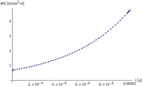
Figure 1. Behavior of the neutron flux $\varphi (t)[n/(c{m}^2.s)]$, supercritical case, over the domain $0\le t\le 10^{-5}$.

Figure 2

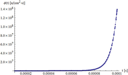
Figure 2. Behavior of the neutron flux $\varphi (t)[n/(c{m}^2.s)]$, supercritical case, over the domain $10^{-5}\le t\le 10^{-4}$.

Figure 3 shows the corresponding behavior of the delayed neutron precursor concentration $C(t)[n/c{m}^2]$ over the interval $0\le t\le 10^{-5}$. The results indicate that the precursor concentration remains nearly unchanged during this initial stage. This is attributed to the relatively low decay constant of the precursors and the short time frame considered, which is insufficient for a noticeable change in the precursor population. While the neutron flux grows rapidly, the precursor response is delayed and follows a slower time scale. These observations are in agreement with the known dynamics of reactor kinetics in supercritical scenarios, particularly under idealized assumptions with no neutron losses. The results also support the effectiveness of the ansatz technique in capturing the early-time behavior of the system.

Figure 3

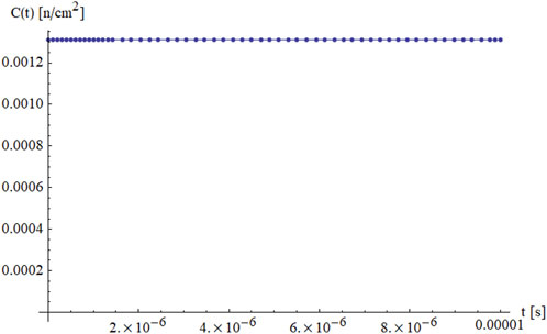
Figure 3. Behavior of the precursor concentration flux $C(t)[n/c{m}^2]$, supercritical case, over the domain $0\le t\le 10^{-5}$.

Figures 4, 5 offer a closer look at how the delayed neutron precursor concentration $C(t)$ evolves during a supercritical transient. In Figure 4, which spans the time interval from $10^{-5}$ to $10^{-4}$ seconds, the concentration begins to rise noticeably after approximately $t=8\times 10^{-5}$ seconds, eventually reaching a value around 0.1 $[n/c{m}^2]$. This gradual response reflects the delayed nature of precursor production, which requires sustained neutron flux to accumulate—a process that lags behind the more immediate growth of the neutron flux observed earlier (as shown in previous figures).

Figure 4

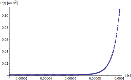
Figure 4. Behavior of the precursor concentration flux $C(t)[n/c{m}^2]$, supercritical case, over the domain $10^{-5}\le t\le 10^{-4}$.

Figure 5

Figure 5. Behavior of the precursor concentration flux $C(t)[n/c{m}^2]$, supercritical case, over the domain $10^{-4}\le t\le 10^{-3.5}$.

In Figure 5, which covers a slightly longer time domain up to $10^{-3.5}$ seconds, the behavior changes significantly. The precursor concentration undergoes rapid exponential growth, exceeding $8\times 10^{16}[n/c{m}^2]$, shortly after $t=3\times 10^{-4}$ seconds. This sharp increase is driven by the sustained high levels of neutron flux, which continually fuel precursor production. Once production dominates over decay, the concentration increases rapidly without bound. While the absolute values reflect an idealized scenario—due to the exclusion of feedback, leakage, or absorption effects. Consequently, the underlying trend is physically consistent with expected supercritical behavior. These results highlight the time-scale separation between prompt and delayed components in reactor kinetics. The neutron flux responds almost instantaneously to changes in reactivity, whereas the precursor population builds up more slowly, only becoming significant after a brief delay. This distinction, evident in both the current and previous figures, reinforces the importance of accounting for delayed neutron dynamics when analyzing transient reactor behavior.

5.2 Critical case

Figure 6 shows how the neutron flux $\varphi (t)$ behaves over a long time period, from $t=0$ to $t=10^5$ seconds, in a critical state for which $\nu {\sum }_f={\sum }_a=3.4\times 10^{-2}$. The flux stays almost constant throughout the entire simulation, settling around the initial value 0.7 $[n/(c{m}^2.s)]$. This indicates that the system is in perfect balance: the number of neutrons produced by fission matches those lost due to absorption or decay. Since Neumann–Neumann boundary conditions are applied, there is no neutron leakage at the boundaries, which means this stable behavior is due only to what’s happening inside the entire system. Figure 7 shows the corresponding trend of the delayed neutron precursor concentration $C(t)$ under the same conditions. Just like the neutron flux, the precursor concentration stays nearly unchanged—around the initial value $\rho {\varphi }_0=0.00112[n/c{m}^2]$—throughout the simulation. This is expected in a critical system, where the production of precursors is balanced by their natural decay, leading to a steady-state condition.

Figure 6

Figure 6. Behavior of the neutron flux $\varphi (t)[n/(c{m}^2.s)]$ , critical case.

Figure 7

Figure 7. Behavior of the precursor concentration flux $C(t)[n/c{m}^2]$ , critical case.

5.3 Sub-critical case

In contrast, Figure 8 presents the sub-critical case, $\nu {\sum }_f=2.85\times 10^{-2}$ , ${\sum }_a=3.0\times 10^{-2}$ , over a shorter period of time, from $t=0$ to $t=50$ seconds. Here, the neutron flux starts at 0.7 $[n/(c{m}^2.s)]$ and decreases gradually, following a clear exponential trend, until it drops to below 0.005 $[n/(c{m}^2.s)]$ . Even though no neutrons escape the domain, the system still shows a steady decline in neutron population. This is simply because the rate of neutron production is not enough to overcome absorption and decay as typical as sub-critical conditions. Figure 9, describes how the precursor concentration changes in the same sub-critical case and time range. It starts at roughly 0.00112 $[n/c{m}^2]$ at $t=0$ , and gradually decreases to less than 0.00005 $[n/c{m}^2]$ by the time $t=50$ seconds. This drop in concentration happens because the lower neutron flux can no longer support the production of precursors, so they just decay over time without being replaced.

Figure 8

Figure 8. Behavior of the neutron flux $\varphi (t)[n/(c{m}^2.s)]$ , sub-critical case.

Figure 9

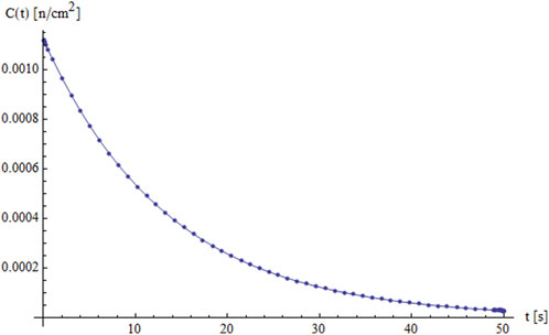
Figure 9. Behavior of the precursor concentration flux $C(t)[n/c{m}^2]$ , sub-critical case.

6 Conclusion

In this paper, a direct ansatz approach was applied to solve the neutron diffusion system under Neumann-Neumann boundary conditions (zero-flux gradient at boundary). An ansatz approach was applied to exactly solve the governing system. Explicit time-dependent solutions were obtained, where spatial variations violate. Detailed physical explanation was discussed for the behavior of the neutron flux and the precursor concentration under the supercritical, the critical, and the sub-critical conditions. Although the methodology is classic, it reflects the simplicity of the ansatz approach to solve the current system under the boundary conditions 3 and 4. The presented simulation cases offer a clear and consistent picture of neutron flux and precursor dynamics across different reactivity conditions. In supercritical scenarios, the model captures the sharp rise in neutron flux and the delayed buildup of precursors, while critical conditions show stable behavior, and sub-critical cases exhibit smooth decay over time. All results align well with theoretical expectations and reflect the core physics of reactor kinetics. The results revealed that the suggested approach was computationally efficient and stable across a wide range of reactivity levels. Overall, the model offers both theoretical clarity and practical utility, making it a useful tool for early-stage reactor design, control analysis, and safety assessment in systems where simplified kinetics are appropriate. Although the present model assumes idealized conditions: no neutron leakage, no feedback mechanisms, one-group approximation and constant parameters, it can be viewed as an application of the ansatz approach to solve a basic neutron diffusion model under zero-flux conditions. To overcome such limitations, the ansatz approach may deserve further extension to analyze other complex forms (realistic reactor scenarios) of the classical/fractional diffusion systems in the spherical and hemispherical reactors in addition to other different geometries subject to various physical factors [40–47].

Data availability statement

The original contributions presented in the study are included in the article/supplementary material, further inquiries can be directed to the corresponding authors.

Author contributions

EE-Z: Conceptualization, Data curation, Formal Analysis, Funding acquisition, Project administration, Supervision, Writing – original draft, Writing – review and editing. AE: Conceptualization, Data curation, Formal Analysis, Investigation, Writing – original draft, Writing – review and editing. LS: Conceptualization, Data curation, Formal Analysis, Methodology, Writing – original draft, Writing – review and editing.

Funding

The author(s) declare that financial support was received for the research and/or publication of this article. “The authors extend their appreciation to Prince Sattam bin Abdulaziz University for funding this research work through the project number (PSAU/2025/01/32274)”.

Conflict of interest

The authors declare that the research was conducted in the absence of any commercial or financial relationships that could be construed as a potential conflict of interest.

Generative AI statement

The author(s) declare that no Generative AI was used in the creation of this manuscript.

Any alternative text (alt text) provided alongside figures in this article has been generated by Frontiers with the support of artificial intelligence and reasonable efforts have been made to ensure accuracy, including review by the authors wherever possible. If you identify any issues, please contact us.

Publisher’s note

All claims expressed in this article are solely those of the authors and do not necessarily represent those of their affiliated organizations, or those of the publisher, the editors and the reviewers. Any product that may be evaluated in this article, or claim that may be made by its manufacturer, is not guaranteed or endorsed by the publisher.

References

1. Lamarsh JR, Baratta AJ. Introduction to nuclear engineering. 3rd ed. Upper Saddle River, NJ: Prentice Hall (2001).

Google Scholar

2. Williams MMR. Mathematical methods in particle transport theory. London: Butterworths (1971).

Google Scholar

3. Bell G, Glasstone S. Nuclear reactor theory. New York: Van Nostrand Reinhold (1970).

Google Scholar

4. Lewis EE, Miller WF. Computational Methods of Neutron Transport. La Grange Park. IL: American Nuclear Society (1993).

Google Scholar

5. Cacuci DG. Handbook of nuclear engineering. In: Nuclear engineering fundamentals, 1. New York: Springer (2010).

Google Scholar

6. Arslan K, Aksan SI. Analytical solutions for transient neutron diffusion in multi-region systems using laplace transforms. Prog Nucl Energy (2019) 115:41–50. doi:10.1016/j.pnucene.2019.03.002

CrossRef Full Text | Google Scholar

7. Ibeid HM, Abu-Mulaweh YS, Kapustin A, Kiselev A, Ryzhov N, Yudina T. Estimation of system code SOCRAT/V3 accuracy to simulate the heat transfer in a pool of volumetrically heated liquid on the basis of BAFOND experiments. Ann Nucl Energy (2021) 151:107902. doi:10.1016/j.anucene.2020.107902

CrossRef Full Text | Google Scholar

8. Ghanavati S, Faghihi F, Dast-Belaraki M. Theoretical study on the passively decay heat removal system and the primary loop flow rate of NuScale SMR. Ann Nucl Energy (2021) 161:108420. doi:10.1016/j.anucene.2021.108420

CrossRef Full Text | Google Scholar

9. Wu H, Stathopoulos A, Orginos K. Multigrid deflation for lattice QCD. J Comput Phys (2020) 409:109356. doi:10.1016/j.jcp.2020.109356

CrossRef Full Text | Google Scholar

10. Taghizadeh M. High-order spectral methods for solving time-dependent neutron diffusion equations. Ann Nucl Energy (2021) 153:108093. doi:10.1016/j.anucene.2021.108093

CrossRef Full Text | Google Scholar

11. Ceolin C, Vilhena MT, Leite SB, Petersen CZ. An analytical solution of the one-dimensional neutron diffusion kinetic equation in Cartesian geometry. In: International Nuclear Atlantic Conference; Janerio, Brazil. INAC (2009).

Google Scholar

12. Khaled SM. Exact solution of the one-dimensional neutron diffusion kinetic equation with one delayed precursor concentration in Cartesian geometry. AIMS Maths (2022) 7(7):12364–73. doi:10.3934/math.2022686

CrossRef Full Text | Google Scholar

13. Nahla AA, Al-Ghamdi MF. Generalization of the analytical exponential model for homogeneous reactor kinetics equations. J. Appl. Math. (2012) 2012:282367. doi:10.1155/2012/282367

CrossRef Full Text | Google Scholar

14. Tumelero F, Lapa CMF, Bodmann BEJ, Vilhena MT. Analytical representation of the solution of the space kinetic diffusion equation in a one-dimensional and homogeneous domain. Braz. J. Radiat. Sci. (2019) 7:01–13. doi:10.15392/bjrs.v7i2B.389

CrossRef Full Text | Google Scholar

15. Nahla AA, Al-Malki F, Rokaya M. Numerical techniques for the neutron diffusion equations in the nuclear reactors. Adv. Stud. Theor. Phys. (2012) 6:649–64.

Google Scholar

16. Khaled SM. Power excursion of the training and research reactor of Budapest university. Int. J. Nucl. Energy Sci.Technol. (2007) 3:43–62. doi:10.1504/IJNEST.2007.012440

CrossRef Full Text | Google Scholar

17. Khaled SM, Mutairi FA. The influence of different hydraulics models in treatment of some physical processes in super-critical states of light water reactors accidents. Int. J. Nucl. Energy Sci. Technol. (2014) 8:290–309. doi:10.1504/IJNEST.2014.064940

CrossRef Full Text | Google Scholar

18. Dulla S, Ravetto P, Picca P, Tomatis D. Analytical benchmarks for the kinetics of accelerator driven systems, joint international topical meeting on mathematics and computation and supercomputing. In: Nuclear applications. Monterey-California, on CD-ROM (2007).

Google Scholar

19. Al-Jeaid HK. A simple approach for explicit solution of the neutron diffusion kinetic system. Maths Stat (2023) 11(1):107–16. doi:10.13189/ms.2023.110112

CrossRef Full Text | Google Scholar

20. Al-Sharif MA, Ebaid A, Alrashdi HS, Alenazy AH, Kanaan NE. A novel ansatz method for solving the neutron diffusion system in cartesian geometry. J Adv Maths Computer Sci (2022) 37(11):90–9. doi:10.9734/jamcs/2022/v37i111723

CrossRef Full Text | Google Scholar

21. Alsubie TMT, Ebaid A, Albalawi ASS, Alghamdi SA, Alhamdi FFM, Alhamd OSH. Developing ansatz method for solving the neutron diffusion system under general physical conditions. Adv Differential Equations Control Process (2024) 31(1):15–26. doi:10.17654/0974324324002

CrossRef Full Text | Google Scholar

22. Dogan N. Solution of the system of ordinary differential equations by combined laplace transform-adomian decomposition method. Math. Comput. Appl. (2012) 17(3):203–11.

CrossRef Full Text | Google Scholar

23. Khaled SM. The exact effects of radiation and joule heating on magnetohydrodynamic marangoni convection over a flat surface. Therm. Sci. (2018) 22:63–72. doi:10.2298/tsci151005050k

CrossRef Full Text | Google Scholar

24. Atangana A, Alkaltani BS. A novel double integral transform and its applications. J. Nonlinear Sci. Appl. (2016) 9:424–34.

Google Scholar

25. Aljohani AF, Ebaid A, Aly EH, Pop I, Abubaker AOM, Alanazi DJ. Explicit solution of a generalized mathematical model for the solar collector/photovoltaic applications using nanoparticles. Alexandria Eng J (2023) 67:447–59. doi:10.1016/j.aej.2022.12.044

CrossRef Full Text | Google Scholar

26. Albidah AB. A proposed analytical and numerical treatment for the nonlinear SIR model via a hybrid approach. Mathematics (2023) 11:2749. doi:10.3390/math11122749

CrossRef Full Text | Google Scholar

27. Venkata Pavani P, Lakshmi Priya U, Amarnath Reddy B. Solving differential equations by using laplace transforms. Int. J. Res. Anal. Rev. (2018) 5(3):1796–9.

Google Scholar

28. Aljoufi MD. Exact solution of a solar energy model using four different kinds of nanofluids: advanced application of laplace transform. Case Stud Therm Eng (2023) 50:103396. doi:10.1016/j.csite.2023.103396

CrossRef Full Text | Google Scholar

29. Aljohani AF, Ebaid A, Algehyne EA, Mahrous YM, Agarwal P, Areshi M, et al. On solving the chlorine transport model via laplace transform. Sci Rep (2022) 12:12154. doi:10.1038/s41598-022-14655-3

PubMed Abstract | CrossRef Full Text | Google Scholar

30. Haberman R. Elementary applied partial differential equations. 2nd ed. USA: Prentice-Hall, Inc (1987).

Google Scholar

31. Liu Y, Sun K. Solving power system differential algebraic equations using differential transformation. IEEE Trans Power Syst (2020) 35:2289–99. doi:10.1109/TPWRS.2019.2945512

CrossRef Full Text | Google Scholar

32. Liao S. Beyond perturbation: introduction to the homotopy analysis method. Boca Raton, FL, USA: CRC Press (2003).

Google Scholar

33. Chauhan A, Arora R. Application of homotopy analysis method (HAM) to the non-linear KdV equations astha chauhan and rajan arora. Commun. Math. (2023) 31:205–20. doi:10.46298/cm.10336

CrossRef Full Text | Google Scholar

34. Nadeem M, Li F. He-Laplace method for nonlinear vibration systems and nonlinear wave equations. J. Low Freq. Noise. Vib. Act. Control. (2019) 38:1060–74. doi:10.1177/1461348418818973

CrossRef Full Text | Google Scholar

35. Nadeem M, Edalatpanah SA, Mahariq I, Aly WHF. Analytical view of nonlinear delay differential equations using sawi iterative scheme. Symmetry (2022) 14:2430. doi:10.3390/sym14112430

CrossRef Full Text | Google Scholar

36. Ayati Z, Biazar J. On the convergence of homotopy perturbation method. J Egypt Math Soc (2015) 23:424–8. doi:10.1016/j.joems.2014.06.015

CrossRef Full Text | Google Scholar

37. Duan JS, Rach R. A new modification of the Adomian decomposition method for solving boundary value problems for higher order nonlinear differential equations. Appl. Math. Comput. (2011) 218:4090–118. doi:10.1016/j.amc.2011.09.037

CrossRef Full Text | Google Scholar

38. Bhalekar S, Patade J. An analytical solution of fishers equation using decomposition method. Am. J. Comput. Appl. Math. (2016) 6:123–7.

Google Scholar

39. Alenazy AHS, Ebaid A, Algehyne EA, Al-Jeaid HK. Advanced study on the delay differential equation y′(t) = ay(t) + by(ct). Mathematics (2022) 10:4302. doi:10.3390/math10224302

CrossRef Full Text | Google Scholar

40. El-Ajou A, Shqair M, Ghabar I, Burqan A, Saadeh R. A solution for the neutron diffusion equation in the spherical and hemispherical reactors using the residual power series. Front. Phys. (2023) 11:1229142. doi:10.3389/fphy.2023.1229142

CrossRef Full Text | Google Scholar

41. Batiha I, Allouch N, Shqair M, Jebril I, Alkhazaleh S, Momani S. Fractional approach to two-group neutron diffusion in slab reactors. Int J Robotics Control Syst (2025) 5(1):611–24. doi:10.31763/ijrcs.v5i1.1524

CrossRef Full Text | Google Scholar

42. Ahmad El-Nabulsi R. Neutrons diffusion variable coefficient advection in nuclear reactors. Int J Adv Nucl Reactor Des Technology (2021) 3:102–7. doi:10.1016/j.jandt.2021.06.005

CrossRef Full Text | Google Scholar

43. Li X, Cheng K, Huang T, Tan S. Research on neutron diffusion equation and nuclear thermal coupling method based on gradient updating finite volume method. Ann Nucl Energy (2024) 195:110158. doi:10.1016/j.anucene.2023.110158

CrossRef Full Text | Google Scholar

44. El-Nabulsi RA. Fractal neutrons diffusion equation: uniformization of heat and fuel burn-up in nuclear reactor. Nucl Eng Des (2021) 380(2021):111312. doi:10.1016/j.nucengdes.2021.111312

CrossRef Full Text | Google Scholar

45. El-Nabulsi RA. Nonlocal effects to neutron diffusion equation in a nuclear reactor. J Comput Theor Transport (2020) 49(6):267–81. doi:10.1080/23324309.2020.1816551

CrossRef Full Text | Google Scholar

46. Phillips TR, Heaney CE, Chen B, Buchan AG, Pain CC. Solving the discretised neutron diffusion equations using neural networks. Int J. Numer Methods Eng. (2023) 124(21):4659–86. doi:10.1002/nme.7321

CrossRef Full Text | Google Scholar

47. Liu D, Liu Y, Dang H, Wang K, Zhang B, Wang F, et al. The neutron transport equation in exact differential form. Sci. China Phys. Mech. Astron. (2025) 68:270511. doi:10.1007/s11433-024-2642-3

CrossRef Full Text | Google Scholar