Multi-subspace mapping and adaptive learning: MMAL-CL for cross-domain few-shot image identification across scenarios

Image detection plays a critical role in quality control across manufacturing and healthcare sectors, yet existing methods struggle to meet real-world requirements due to their heavy reliance on large labeled datasets, poor generalization across different domains, and limited adaptability to diverse application scenarios. These limitations significantly hinder the deployment of AI solutions in practical industrial settings where data scarcity and domain variations are common. To address these issues, we propose MMAL-CL, a unified deep learning framework that integrates an Edge Feature Module (EFM) with multi-subspace mapping attention and an Adaptive Deep Learning Module (ADLM) for cross-domain feature decoupling. The EFM extracts translation-invariant features through residual convolution blocks and a novel multi-subspace attention mechanism, enhancing the model’s ability to capture interdependencies between features. The ADLM enables few-shot learning by mixing task-irrelevant auxiliary data with target domain samples and optimizing feature separation via a dual-classifier strategy. Finally, we evaluated the model’s performance on five datasets (two industrial and three medical) demonstrate that MMAL-CL achieves 99.7% precision on the NEU-CLS dataset with full data and maintains 71.3% precision with only 20 samples per class, outperforming other methods in few-shot settings. The framework shows remarkable cross-domain generalization capability, with an average 12.8% improvement in F1-score over existing methods. These results highlight MMAL-CL’s potential as a practical solution for image detection that can operate effectively with limited training data while maintaining high accuracy across diverse application scenarios.

1 Introduction

Image identification and classification have emerged as fundamental technologies supporting modern industrial systems and quality control processes [1, 2]. These techniques enable automated identification and analysis of critical features in manufacturing inspection, medical diagnosis, and other application domains [3]. The integration of machine learning with neural networks has significantly advanced this field, driving progress in diverse areas ranging from precision surface defect identification to complex medical image analysis [4–6]. However, as industrial applications diversify, current deep learning-based solutions reveal some challenges that demand urgent attention. Although these methods have achieved good performance under certain conditions, traditional image identification methods rely on manually designed feature extraction methods, so that image identification is limited by the quality of feature selection and design, resulting in limited identification performance of the model [7–10]. Compared with the time-consuming and labor-intensive traditional methods, deep learning-based methods have gradually become a research hotspot in the field of image identification due to its robust feature recognition capabilities and high accuracy [11–15].

With the outstanding performance of AlexNet in the 2012 ImageNet competition, it successfully opened a new chapter in deep learning in the field of image identification [16–20, 27]. Many studies have demonstrated that AI technology has broad application prospects in medical diagnosis, industrial identification and other fields. In terms of image identification, Yu et al. proposed a RegNet that can identify sewer pipe defects. The model uses dropout to improve the overfitting problem of the model and uses LeakyReLU to further optimize the performance of the model [21]. Joon-Hyung et al. summarized the characteristics of industrial PCB images, analyzed the factors that may cause image data changes in the industrial field, and proposed a convolution-based PCB defect identification method on this basis [22]. Said et al. proposed a ResNet model based on transfer learning, which can use pathological images to diagnose whether a patient has breast cancer [23]. Sasank et al. built a model based on a deep residual network that can analyze the patient’s brain health based on CT images [24]. Gabriele et al. proposed a weakly supervised deep learning framework based on convolutional networks, which can analyze cancer based on whole slide pathological images [25]. In additional, deep learning technology has received widespread attention due to its ability to achieve performance similar to human experts in a short period of time [26, 27]. Jun et al. also proposed a data augmentation and weight allocation method to solve the problem of insufficient samples and uneven sample distribution [28]. Xiao et al. proposed a model for assisting in the diagnosis of COVID-19 using CT images. The model uses contrastive learning to train the encoder to capture the necessary features on large-scale datasets, to reduce the model’s demand for the quantity of raw data [29]. Tae Keun et al. proposed a feasibility study method, which improves the performance of the model in small-scale samples through data amplification [30]. Ling et al. proposed a DLA-MatchNet, which integrates channel attention, spatial attention and feature networks to enable it to handle small amounts of data samples [55].

Despite their demonstrated potential, current deep learning-based identification methods still have limitations. A primary challenge stems from the substantial data dependence of these models. Variations in imaging devices and acquisition protocols across different facilities often lead to significant domain shifts, resulting in poor generalization performance when applying models to new clinical or industrial settings. While data augmentation strategies can partially mitigate this issue, collecting large-scale annotated datasets remains prohibitively expensive in many real-world scenarios. This is particularly evident in medical imaging, where patient privacy concerns restrict data availability, and in industrial inspection systems, where rare defects are inherently difficult to capture. Furthermore, existing approaches are typically designed for specific application domains, with limited transferability across different identification tasks. This domain specificity necessitates the development of specialized models for each application scenario, significantly increasing deployment costs and complexity. Although transfer learning techniques have shown promise in reducing data requirements, they still rely heavily on the availability of relevant source domain data. In practice, the requirement for semantically similar pre-training data often cannot be satisfied, particularly for novel or rare defect types. In order to alleviate the above problems, transfer learning was proposed. Although these studies have achieved many breakthroughs, they still need to be further optimized. Transfer learning typically uses similar data to pre-train the model for a target task. However, in reality, similar data is often difficult to obtain. More and more visual tasks are showing a need to reduce the number of training samples [31–34]. Architectural limitations of conventional CNNs present additional challenges. The local receptive fields of convolutional operations constrain the model’s ability to capture long-range feature dependencies, while simply increasing network depth leads to prohibitive computational costs. Recent studies have shown that attention mechanisms can improve feature learning, but most implementations fail to maintain an optimal balance between performance and computational efficiency, especially in resource-constrained industrial environments.

To solve the above problems, this paper proposes a novel deep learning-based image identification method and with the following contributions. First, we develop a unified deep learning architecture that integrates multi-scale feature extraction with attention mechanisms, enabling high-precision identification while maintaining computational efficiency. This design effectively balances model performance and resource requirements. Second, the proposed model significantly reduces data requirements through an innovative few-shot learning paradigm. Third, our solution introduces a scenario-adaptive mechanism that automatically adjusts feature representation according to different application domains. This innovation enables seamless deployment across diverse industrial and medical scenarios without architectural modifications. Fourth, we introduce a cross-domain learning mechanism that utilizes task-irrelevant auxiliary data. This component enhances model generalization while optimizing storage and computation costs. Finally, we propose a multi-subspace attention module that overcomes the limitations of conventional CNNs. The principle of the framework proposed is illustrated in Figure 1.

Figure 1

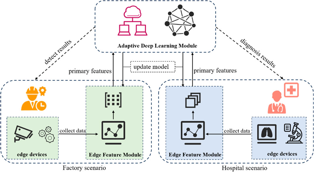
Figure 1. Workflow of proposed framework.

2 Methods

This section presents the technical details of MMAL-CL, a unified framework designed for multi-scenario image identification in both medical and industrial scenarios. As illustrated in Figure 1. MMAL-CL mainly includes Edge Feature Module (EFM) and Adaptive Deep Learning Module (ADLM). Firstly, the edge devices in each scenario will collect the required data, which is then be feed into the EFM to obtain edge primary features. And then the edge features will be sent to the ADLM for scenario allocation and feature identification. The aforementioned scenario allocation means that the ADLM will send information to the corresponding neural network based on the data source. After obtaining the feature identification results, the ADLM will return the results to the doctor or engineer and update the network parameters of the EFM according to the needs. Next, we will describe the model construction method in detail.

2.1 Edge feature module

Edge Feature Module is responsible for automatically extracting primary features of scenario data at each edge devices, including pathological images collected from hospitals and steel surface images collected from factories. In order to make the model easier to converge, we will use an auxiliary dataset to initialize its parameters, as shown in Figure 2.

Figure 2

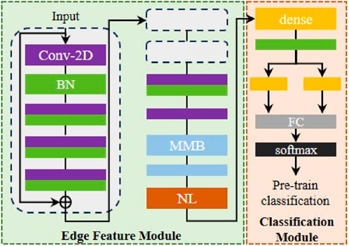
Figure 2. Workflow of proposed framework. EFM parameter initialization schematic diagram (Conv-2D means 2D convolution layer, BN means batch normalization, MMB means multi-subspace mapping block, NL means normalization, FC means fully connection layer. The same color represents the same layer).

We use Mini-ImageNet as initialization auxiliary samples. It is worth noting that the samples used in pre-training are target-independent data, which is consistent with the original intention mentioned above. In the initial parameter initialization stage, task-independent auxiliary data will be sent to the EFM to obtain potential features, and then the above features will be used by the classification module (CM) to obtain the classification results. When the expected classification performance is obtained in the auxiliary dataset, the pre-training phase is completed, and the EFM will be taken out and embedded into the edge server and the cloud.

Specifically, EFM mainly consists of convolution block and multi-subspace mapping block (MMB). The convolution block is designed as a residual structure, which consists of convolution layers and batch normalization. The residual structure helps improve the ability of model to learn different scales features and improve the fluidity of gradients. After being processed by the residual convolution block, the information will be fed into the convolution layer to further refine the required features. Afterwards, the feature map will be sent to MMB, and the principle is shown in Figure 3.

Figure 3

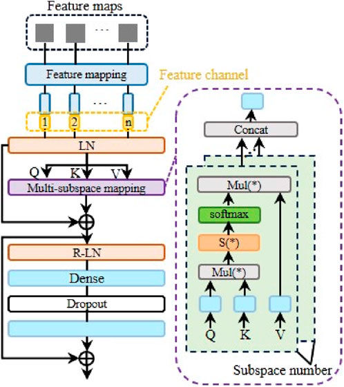
Figure 3. Multi-subspace mapping block schematic Workflow of proposed framework.

To make the model can learn feature dependencies, this paper designs a data analysis structure based on self-attention, inspired by the transformer. After obtaining the feature maps from the above convolution layer, the model will linearly map these feature maps. This step allows the model to adjust input information more flexibly according to target requirements, allowing the model to converge more robustly. In addition, to a certain extent, this step can also be regarded as a process of appropriately mixing noise, which can improve the robustness of the model. After the feature mapping process, the feature maps will be converted into feature vectors. At this point, we embed the feature channel encoding into the corresponding feature vector. Feature encoding represents the identity information of different feature channels, which helps the model learn the interdependence between different features. The embedded feature vector will be sent to the LN layer. LN refers to layer normalization. The principle is shown in Equation 1.

$\mathit{LN}\left(efv\right)=GeLu\left(\frac{{\beta }_1}{\sqrt{{\sigma }^2+\theta }}\odot \left(efv-\overline{efv}\right)+{\beta }_2\right)(1)$

Among them, efv represents the above-mentioned embedded feature vector, GeLu (*) represents the activation function GeLu, ${\beta }_1$ and ${\beta }_2$ are learnable parameters, $\sigma$ is the variance, $\theta$ is the minimum value to ensure that the fraction is meaningful, and $\overline{efv}$ is the average of efv. As shown in Equation 1, layer normalization is not affected by the data batch size. Compared to the classical batch normalization whose performance is limited by the batch size, LN can provide more stable statistics for the model, thus making its convergence process more robust. After this, the corresponding vector will be fed into multi-subspace mapping layer. $Q,\mathrm{K},\mathrm{V}$ are three input channels respectively, each with independent mapping parameters, as shown in Equation 2.

$Q^{\prime }={\theta }_{Q}Q{K}^{\prime }={\theta }_{K}K{V}^{\prime }={\theta }_{V}V(2)$

Here, ${\theta }_{\left(*\right)}$ is the mapping parameter of the respective channel, and ${\mathrm{Q}}^{\prime },{\mathrm{K}}^{\prime },{\mathrm{V}}^{\prime }$ are the mapped channel vectors respectively. Independent mapping parameters can not only improve the flexibility of the model, but can also be regarded as the mapping of the same input in different feature spaces to a certain extent, which helps to improve the robustness of the model. After mapping, ${\mathrm{Q}}^{\prime }$ and ${\mathrm{K}}^{\prime }$ will be dot producted, as shown in Equation 3.

$Mul\left(Q^{\prime },K^{\prime }\right)=Q^{\prime }{K^{\prime }}^T(3)$

In order to suppress the variance and avoid the difficulty of model learning caused by the vanishing gradient, we further perform a scaling operation based on Equation 3, which corresponds to S (*) in Figure 3. The principle is shown in Equation 4.

$S\left(Mul\left(Q^{\prime },K^{\prime }\right)\right)=\frac{Mul\left(Q^{\prime },K^{\prime }\right)}{\sqrt{O_Q}}(4)$

Here, ${\mathrm{O}}_{\mathrm{Q}}$ is the dimension of the input vector Q. Combining Equations 3, 4, the role of the dot product operation is to learn the interdependence between features. After processed by S (*), we can use the softmax function to obtain the weights assigned to different features by the model. Based on the above weights, the output of a single subspace can be obtained by weighting the feature expression, as shown in Equation 5.

$space\left(Q^{\prime },K^{\prime },V^{\prime }\right)=softmax\left(S\left(Mul\left(Q^{\prime },K^{\prime }\right)\right)\right)V^{\prime }(5)$

Where, space (*) represents the output of a single subspace. By splicing the outputs of multiple subspaces and assigning corresponding weights, the final output of the multi-subspace mapping layer can be obtained, as shown in Equation 6.

$MML\left(Q^{\prime },K^{\prime },V^{\prime }\right)=f\left({space}_1,{space}_2,\dots ,{space}_n\right){\theta }_{mml}(6)$

In the equation, $MML\left(*\right)$ is the output of multi-subspace mapping layer, f (*) represents the splicing operation, spacen represents the output of the nth subspace, ${\theta }_{mml}$ is the corresponding parameter. Because it combines the output of multiple feature spaces, it is called a multi-subspace mapping layer.

As mentioned above, in order to improve the model’s ability to grasp features of different scales, this paper also designs residual links. As shown in Figure 3, after passing through the multi-subspace mapping layer, the data will also be processed by the residual normalization layer, as shown in Equation 7.

$R\_\mathit{LN}\left(x\right)=\mathit{LN}\left(x+MML\left(x\right)\right)(7)$

Here, $\mathrm{R}\_\mathrm{LN}\left(*\right)$ represents the R-LN layer output, and x represents the channel-embedded feature vector. As shown in Figure 3, after being processed by the dense layer and dropout layer, the final output of MMB can be obtained.

After two consecutive MMB processes, the feature vector will be normalized and then sent to the CM. As shown in Figure 2, CM is a classic classification network. In the pre-training stage, the role of CM is to classify the auxiliary data. By training a classification model, it determines a good initial weight for EFM. The loss function of CM is cross-entropy. Compared with the mean square error, cross-entropy is not affected by the gradient of the activation function, which can avoid the problem of vanishing gradient to a certain extent and make the model easier to converge.

2.2 Adaptive deep learning module

Adaptive Deep Learning Module is responsible for using task-independent data to assist the model in learning the target task. This can reduce the data scale for achieving the expected performance of the model in this paper, save storage space and deployment costs, and improve the model’s generalization ability for multi-center or multi-scenario data, thereby accelerating the further extension of AI-based image identification applications. It is worth noting that ADLM uses task-independent data to assist model learning instead of similar data, which reduces the model’s dependence on original data to a certain extent. The principle of ADLM is shown in Figure 4.

Figure 4

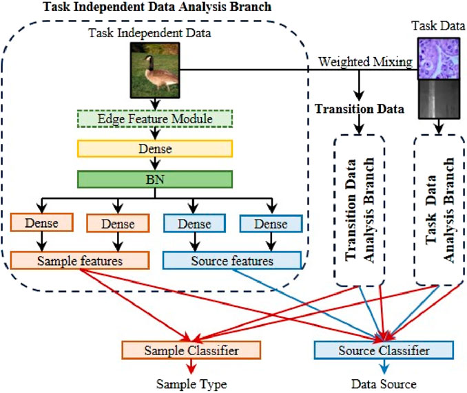
Figure 4. Adaptive deep learning module principal diagram.

We hope that the model can use task-independent data to assist itself in learning target data, but there are huge domain differences between data in different fields, which will make model learning difficult. To alleviate this problem, we mixed task independence data and task data to form transition data to alleviate the problem of difficulty in understanding domain differences. The mixing principle is shown in Equation 8.

$TRD\left({TD}_{\left(m\right)},{TID}_{\left(n\right)}\right)=\phi ·{TD}_{\left(m\right)}+\left(1-\phi \right)·{TID}_{\left(n\right)}(8)$

Where, TRD is transition data, TD(m) represents the random mth type sample in task data, TID(n) represents the nth type of sample in task independent data, $\mathrm{\phi }$ is the mixing parameter. $\phi \sim beta\left(\epsilon ,\epsilon \right)$, here, $\epsilon \subseteq \left(0,\infty \right)$. The transition samples only involve mutual mixing between single-class samples, and do not involve cross-mixing of multi-class samples.

As shown in Figure 4, the three types of samples are sent to three branches respectively. Among them, the structures of transition data analysis branch and task data analysis branch are the same as task independent data analysis branch. After obtaining relevant information, the sample features are sent to the sample classifier. The function of this classifier is to identify the type of target data, that is, to output the disease type or part surface defect type. The sample features and source features are fed into the source classifier. The function of the classifier is to identify the source of the data, that is, whether the data comes from the target data or auxiliary data. The purpose of designing two classifiers is to enable the model to automatically decouple sample features and source features. In other words, this design approach allows the model to separate features that are similar to the target task (sample features) and features that are not highly correlated to the target task (source features) from the task independent data. This is because sample features can determine the sample type, so it can be considered relevant to the target task. On the contrary, source features can determine the source of the sample, so it contains huge domain bias and is quite different from the target task. When processing transition data and task data, the model classifies them separately based on the categories of their respective datasets, obtaining classification losses $L_{TD}$ and $L_{TID}$. Because it is a classic classification model, the above two losses are cross-entropy. As stated in Equation 8, the transition data is a mixture of the above two types of data, so the loss function of the sample classifier can be expressed as Equation 9. Where, $L_{SC}$ is the loss function of the sample classifier.

$L_{SC}=\phi ·L_{TD}+\left(1-\phi \right)·L_{TID}(9)$

Source classifier is responsible for identifying the source of the data. Based on the above, we hope that the sample classifier can separate potential features that are closely related to the target task in task-irrelevant data, while the source classifier is intended to distinguish domain-specific differences. To achieve the above functions, we designed a special loss function for the source classifier. We want the sample feature to be domain-independent, so the goal of the sample feature is to confuse the source classifier. When the classifier uses sample feature, the labels of all corresponding samples are 0.5, and the loss function is shown in Equation 10.

$\begin{array}{c}{L}_{SOU{C}_{TD}}=\frac{1}{3N}{\displaystyle \sum _x^{\hspace{0.17em}}}[KL\left(SOUC\left({\widehat{y}}_{TID}\right),label\right)+KL\left(SOUC\left({\widehat{y}}_{TRD}\right),label\right)\\ \left.+KL\left(SOUC\left({\widehat{y}}_{TD}\right),label\right)\right]\end{array}(10)$

Here, KL (*) is KL divergence, N is sample size, SOUC(*) is the output of the source classifier, and label refers to the aforementioned label, ${\widehat{y}}_{TID},{\widehat{y}}_{TRD},{\widehat{y}}_{TD}$ are the outputs of task independent data analysis branch, transition data analysis branch, and task data analysis branch respectively. When the classifier processes source features, it is expected to be able to distinguish data sources, and the loss function is shown in Equation 11.

$\begin{array}{c}{L}_{SOU{C}_{TID}}=\frac{1}{3}[CE\left(SOUC\left({\widehat{y}}_{TID}\right),l_{TID}\right)+CE\left(SOUC\left({\widehat{y}}_{TD}\right),l_{TD}\right)+\phi ·\\ CE\left(SOUC\left({\widehat{y}}_{TRD}\right),l_{TD}\right)+\left(1-\phi \right)·CE\left(SOUC\left({\widehat{y}}_{TRD}\right),l_{TID}\right)\end{array}(11)$

Here, CE (*) is cross-entropy, $l_{TID}$ and $l_{TD}$ are data source labels, corresponding to task independent data and task data respectively. Finally, the overall loss function of the model can be written as follows in Equation 12.

$L=L_{SC}+L_{SOUC\_TD}+L_{SOUC\_TID}(12)$

Finally, ADLM will return recognition results to terminal devices located in different scenarios and return model parameters to EFM. Through the above method, the model proposed can adapt to different data analysis needs in various scenarios, including hospitals and factories, by using the same auxiliary data. At the same time, this method also reduces the amount of data required for the model, saves deployment costs, improves the model’s generalization ability for multi-center or multi-scenario data, and accelerates the further extension of AI-based image identification applications.

3 Experiment and discussion

In this section, we primarily describe the experimental data and evaluate the performance of our proposed model using precision, recall, and F1-score as the evaluation metrics. Additionally, we analyze and discuss the experimental results. The proposed approach is implemented by Pytorch on a workstation with NVIDIA GeForce GTX2080Ti.

3.1 Data description

In this paper, we use five datasets from different scenarios, including two factory datasets (NEU-CLS and SEVERSTAL) [35, 36] and three hospital datasets [37–39]. In addition, in order to explore the identification ability of our model on small-scale samples, we extracted 5, 10, and 20 samples per class from all datasets for training. These correspond to 5-data, 10-data and 20-data respectively. Specifically, 5-data refers to randomly selecting five samples from each type of data, and the remaining data is used as the test set. The corresponding extraction methods for 10 and 20 are the same. Mini-ImageNet [40] is a universal pre-training data. The experimental result is the average of five repeated experiments.

3.2 Results and analysis

We demonstrate the performance of our model and conduct many comparative experiments. For the factory scenario, the model performance is shown in Table 1 and Figure 5. The confusion matrix is shown in Supplementary Appendix Figures A1–A6. Here, task a is NEU-CLS and task b is SEVERSTAL. The methods of comparison include AlexNet [41], VGG19 [42], RESNET50 [43], INCEPTION [44], DPN92 [45], Transformer [46].

Table 1

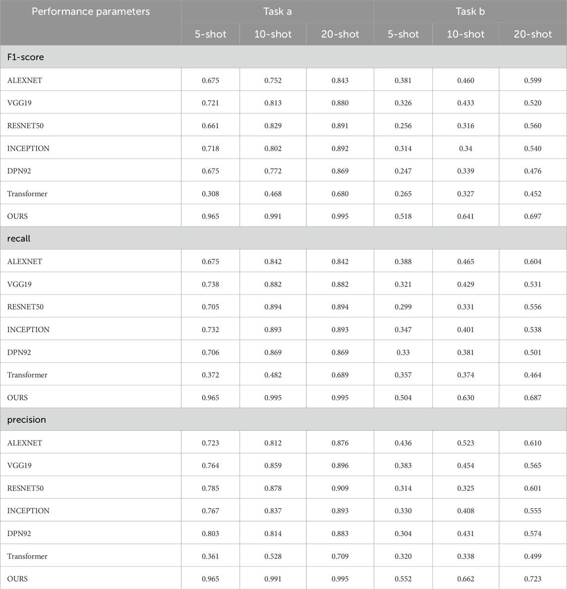
Table 1. The performance of each model in the factory scenario for different sample sizes in tasks a and b, where task a and task b represent NEU-CLS and SEVERSTAL respectively, OURS represents MMAL-CL.

Figure 5

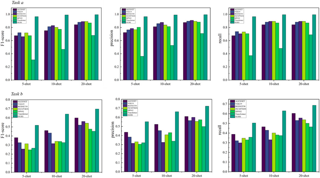
Figure 5. Model’s performance in the factory scenario.

From the experimental results, the framework of this paper achieves better performance. Even though all comparison methods also use relevant data for pre-training, they still do not exceed the proposed framework. We speculate that the reason for this phenomenon is that the feature decoupling structure designed in this paper allows the model to mine potentially valuable information in task-irrelevant data to assist its own learning. The performance of the model based on ResNet is higher than the classic convolutional network VGG. This situation illustrates the necessity of designing the residual structure in this paper. The residual structure helps improve the model’s ability to learn features of different scales. The performance of Transformer is also lower than ResNet, which also proves the necessity of the feature extraction module designed in this paper. It can effectively alleviate the difficulty of Transformer in learning translation invariance. In addition, the performance of ResNet does not exceed the proposed model. The reason for this may be that the MMB can effectively alleviate the difficulty of CNN in learning feature dependencies. The existence of a single structure can be further enhanced [47–49].

For the hospital scenario, we used data from three centers, including five tasks, namely, task a (assessing benign or colon cancer with colon tissue), task b (assessing the lung squamous cell carcinoma, lung adenocarcinoma or benign with lung tissue), task c (assessing the tumor, inflammation or benign with colon tissue), task d (assessing lobular carcinoma, mucinous carcinoma and papillary carcinoma) and task e (assessing adenosis, fibroadenoma, phyllodes tumor, tubular adenoma). The model performance is shown in Table 2 and Figure 6. The confusion matrices are shown in Supplementary Appendix Figures A7–A24. The methods of comparison include PROTO [50], ANIL [51], MAML [52], DN4 [53].

Table 2

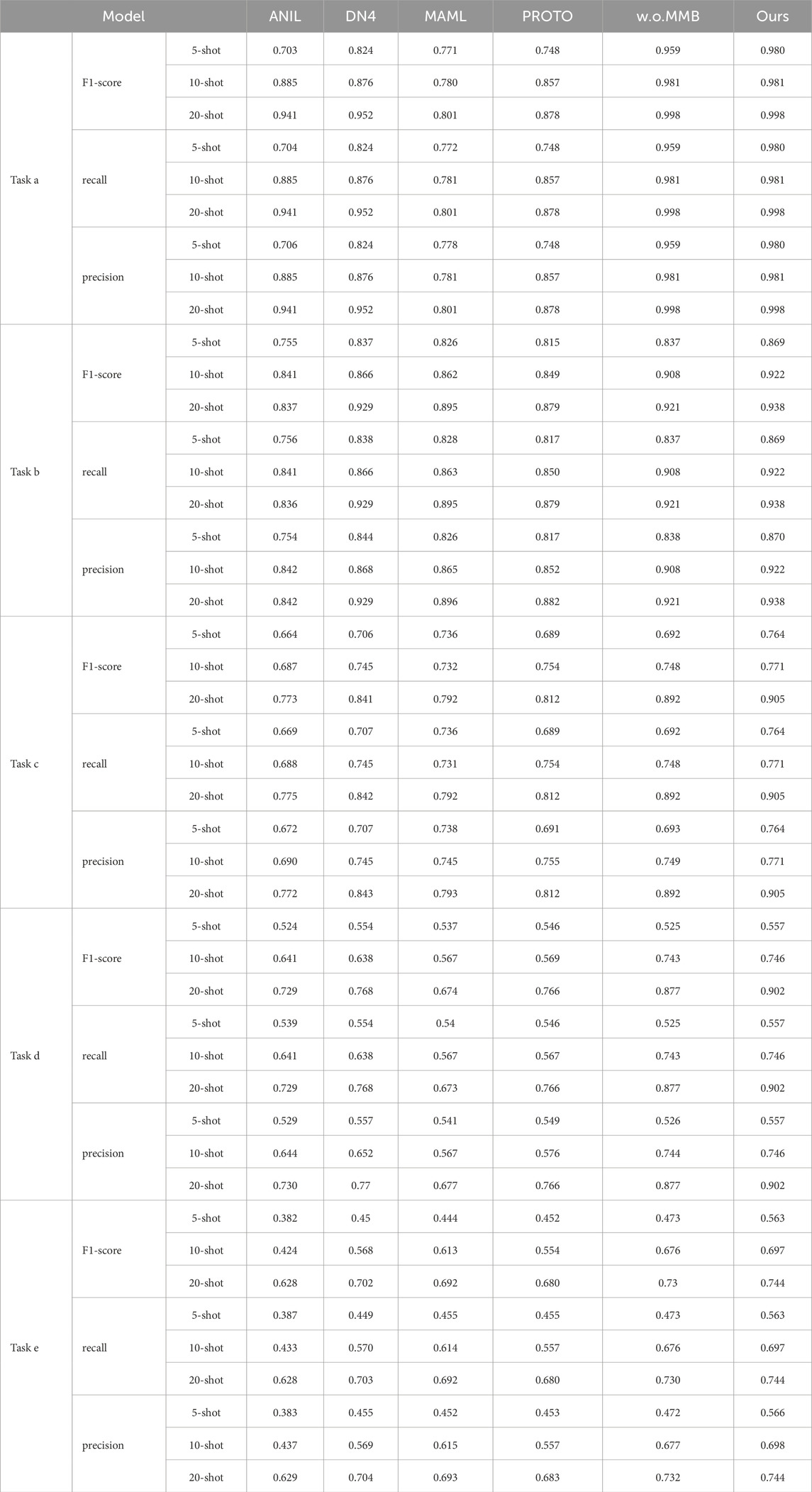
Table 2. The performance of each model in the hospital scenario for different numbers of sample size in tasks a, b, c, d and e, where ours represents MMAL-CL.

Figure 6

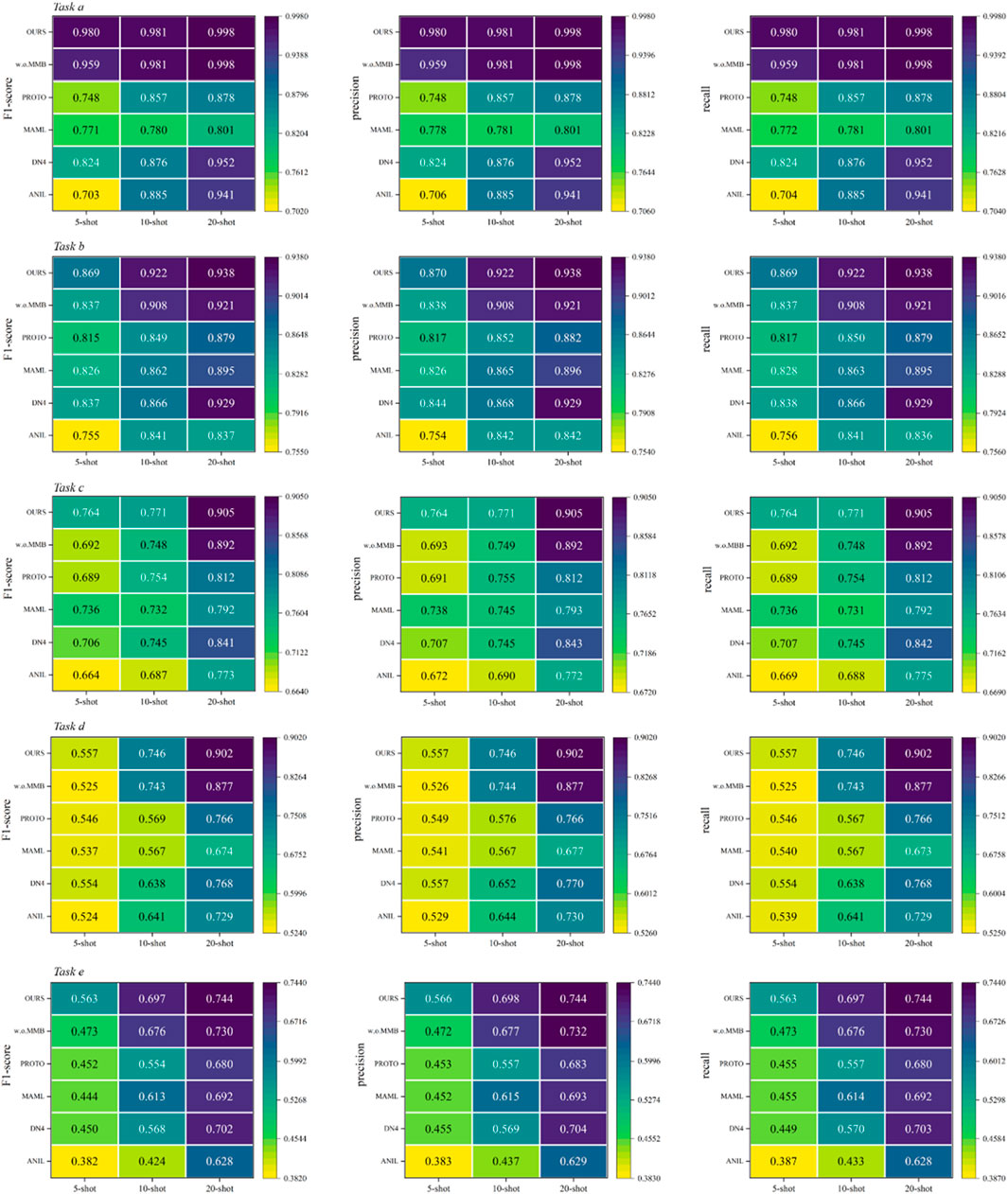
Figure 6. Model’s performance of task a, b, c, d and e in the hospital scenario.

It can be seen from the experimental results that compared with other methods, the proposed method has advantages in various evaluation indicators. We speculate that this is because models based only on convolution are difficult to mine useful information from task-unrelated data to assist their own learning. Therefore, when faced with lightweight data, the models have difficulty in demonstrating good generalization ability. At the same time, the performance of w. o. MMB does not exceed the proposed model. Here, w. o. MMB refers to replacing MMB with convolutional layers, using only the feature decoupling strategy proposed in this paper. This experimental phenomenon once again proves that the MMB designed can effectively alleviate the problem that classic convolutional networks are difficult to learn feature dependencies. In addition, compared with other models, this method does not suffer from task differences in performance. This also confirms the above viewpoint that the multi-subspace mapping method designed in this paper enables the model to master different expression forms of feature.

Representation, thereby enhancing the robustness of the model. Meanwhile, it can be noted that the performance of the model in tasks d and e is limited. We speculate that there may be the following reasons. First, Task e involves four pathological categories and Task d includes three carcinoma subtypes, whereas Task a (2 categories) and Task b (3 less overlapping categories) have fewer or more distinguishable classes. More categories increase inter-class feature overlap, making it harder for the model to learn discriminative representations. Second, potential subtle class imbalance and finer-grained pathological differences further challenge feature decoupling. Thirdly, The difficulty of obtaining high-quality medical samples is usually high, so image quality is also one of the reasons for this phenomenon. How to further improve the performance of the model is our main research work in the future.

The performance of different models in cross scenario scenarios is also compared. In order to express the results concisely, the F1 score had been chosen for comparison, which can objectively represent the comprehensive performance of the model. Meanwhile, we conducted a comparison of model stability by randomly selecting samples and repeating the experiment five times, the results as shown in Table 3. The methods of comparison include DLA-MatchNet [54], LFT [55].

Table 3

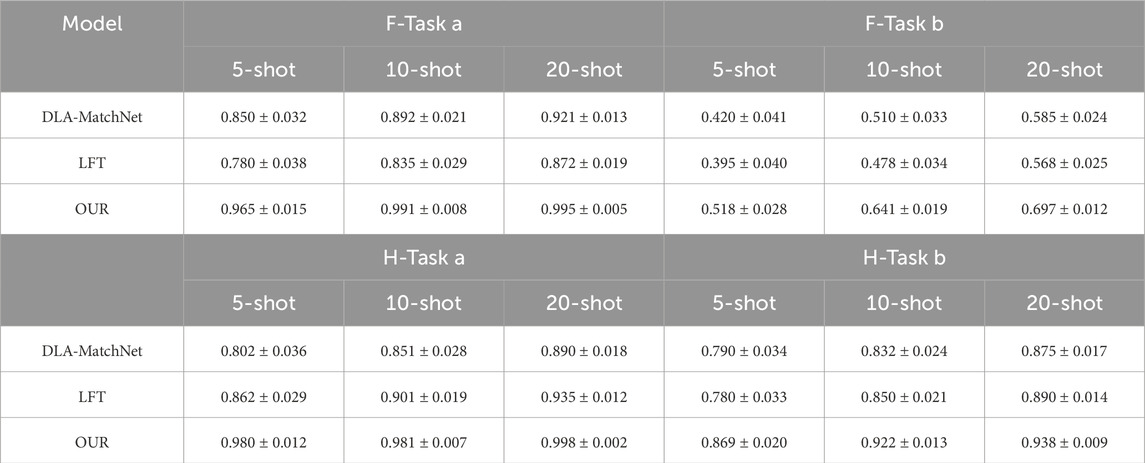
Table 3. Cross scenario performance validation, where F-Task a and F-Task b represent Task a and b in industrial scenarios,H-Task a and H-Task b represent Task a and b in hospital scenarios.

The core challenge of cross-domain few-shot detection is to maintain stable performance when scenarios switch. MMAL-CL achieves this goal through the unified framework of “EFM + ADLM”. As shown in the experimental results, the LFT model outperforms traditional models but lags behind DLA-MatchNet and MMAL-CL. This confirms that feature transformation can alleviate domain shift; however, the multi-subspace attention (EFM) and adaptive feature disentanglement (ADLM) proposed in this paper can achieve more accurate cross-domain feature alignment. Meanwhile, this experimental phenomenon covers both industrial and medical scenarios. Such consistency verifies that the multi-subspace attention (EFM) (which captures cross-scale feature dependencies) and adaptive feature disentanglement (ADLM) (which separates domain-invariant features) of MMAL-CL can effectively address scenario-specific challenges without modifying the model architecture. Second, even under the 5-shot setting where data is most scarce, the method proposed in this paper still achieves acceptable performance. This indicates that the method can mine task-related information from task-irrelevant auxiliary data via ADLM, reduce reliance on target domain samples, and thus exhibits low sensitivity to the number of samples. Additionally, MMAL-CL maintains a low standard deviation in both industrial and medical scenarios, which proves that the proposed method possesses a certain degree of robust adaptability to different data distributions.

Combined with the experimental results of the above two scenarios, our framework shows better performance in multiple application scenarios and multiple data centers. This model is applicable to multiple scenarios, including hospitals and factories. With only a small amount of data, the model can achieve acceptable performance. The model achieves different performances in different tasks, we speculate that this is due to variations in data quality collected by different edge devices. At the same time, the model proposed uses the same auxiliary data for different application scenarios, without having to re-find different auxiliary data according to task requirements, which further increases the potential of the framework to be applied.

4 Conclusion

This paper proposes MMAL-CL, a novel unified deep learning model for cross-domain image identification that addresses challenges in current systems. First, our cross-domain learning mechanism establishes a principled approach for decoupling domain-invariant and domain-specific features through a dual-pathway design. This enables effective knowledge transfer from task-irrelevant auxiliary data while preventing negative transfer, as demonstrated by consistent performance across medical and industrial testbeds.

Second, the unified feature representation framework achieves significant improvements in both data efficiency and deployment flexibility. The system maintains robust performance with limited training samples through its hybrid attention-convolution feature extractor and adaptive scenario allocation module. In addition, when faced with multiple data centers, the model can still provide auxiliary analysis results stably and efficiently without the need to retrain after collecting a large amount of data. Meanwhile, the proposed method can use the same task-independent dataset to assist the model in learning target tasks in different scenarios, further paving the way for the development of the AI-based devices. From the experimental results, in multiple datasets and application scenarios (including hospitals and factories), our method has achieved better performance. This proves that the method proposed in this paper has better robustness to a certain extent. The next step is to further improve the model’s ability to mine data features and explore its auxiliary capabilities for more application scenarios.

Data availability statement

The original contributions presented in the study are included in the article/Supplementary Material, further inquiries can be directed to the corresponding author.

Ethics statement

Ethical approval was not required for the studies involving humans because all biological data used are from publicly available datasets. The studies were conducted in accordance with the local legislation and institutional requirements. The human samples used in this study were acquired from all biological data used are from publicly available datasets. Written informed consent to participate in this study was not required from the participants or the participants’ legal guardians/next of kin in accordance with the national legislation and the institutional requirements.

Author contributions

QD: Conceptualization, Validation, Visualization, Writing – original draft, Writing – review and editing. XX: Conceptualization, Validation, Writing – review and editing. QL: Conceptualization, Validation, Writing – review and editing. YL: Conceptualization, Funding acquisition, Validation, Visualization, Writing – review and editing. LL: Conceptualization, Validation, Writing – review and editing. ZM: Conceptualization, Project administration, Validation, Writing – review and editing.

Funding

The author(s) declare that financial support was received for the research and/or publication of this article. This paper was supported by National Key Research and Development Program of China (2024YFB3312904).

Acknowledgments

The authors thank the reviewers and editors for their comments and suggestions.

Conflict of interest

The authors declare that the research was conducted in the absence of any commercial or financial relationships that could be construed as a potential conflict of interest.

Generative AI statement

The author(s) declare that no Generative AI was used in the creation of this manuscript.

Any alternative text (alt text) provided alongside figures in this article has been generated by Frontiers with the support of artificial intelligence and reasonable efforts have been made to ensure accuracy, including review by the authors wherever possible. If you identify any issues, please contact us.

Publisher’s note

All claims expressed in this article are solely those of the authors and do not necessarily represent those of their affiliated organizations, or those of the publisher, the editors and the reviewers. Any product that may be evaluated in this article, or claim that may be made by its manufacturer, is not guaranteed or endorsed by the publisher.

Supplementary material

The Supplementary Material for this article can be found online at: https://www.frontiersin.org/articles/10.3389/fphy.2025.1681254/full#supplementary-material

Abbreviations

DL, Deep Learning; CNN, Convolutional Neural Networks; BN, Batch Normalization; CM, Classification Module; ADLM, Adaptive Deep Learning Module; EFM, Edge Feature Module.

References

1. Bajić F, Job J. Review of chart image detection and classification. Int J Document Anal Recognition (Ijdar) (2023) 26(4):453–74. doi:10.1007/s10032-022-00424-5

CrossRef Full Text | Google Scholar

2. Liu L, Ouyang W, Wang X, Fieguth P, Chen J, Liu X, et al. Deep learning for generic object detection: a survey. Int J Comput Vis (2020) 128:261–318. doi:10.1007/s11263-019-01247-4

CrossRef Full Text | Google Scholar

3. Sharma S, Bhatt M, Sharma P. Face recognition system using machine learning algorithm[C]. In: 2020 5th international conference on communication and electronics systems (ICCES). IEEE (2020). p. 1162–8.

Google Scholar

4. Chowdhury A, Kautz E, Yener B, Lewis D. Image driven machine learning methods for microstructure recognition. Comput Mater Sci (2016) 123:176–87. doi:10.1016/j.commatsci.2016.05.034

CrossRef Full Text | Google Scholar

5. Lai Y. A comparison of traditional machine learning and deep learning in image recognition. J Phys Conf Ser IOP Publishing (2019) 1314(1):012148. doi:10.1088/1742-6596/1314/1/012148

CrossRef Full Text | Google Scholar

6. Ahammed MT, Ghosh S, Ashik MAR. Human and object detection using machine learning Algorithm[C]//2022 trends in electrical, electronics. In: Computer engineering conference (TEECCON). IEEE (2022). p. 39–44.

CrossRef Full Text | Google Scholar

7. Wang P, Fan E, Wang P. Comparative analysis of image classification algorithms based on traditional machine learning and deep learning. Pattern recognition Lett (2021) 141:61–7. doi:10.1016/j.patrec.2020.07.042

CrossRef Full Text | Google Scholar

8. Rani P, Kotwal S, Manhas J, Sharma V, Sharma S. Machine learning and deep learning based computational approaches in automatic microorganisms image recognition: methodologies, challenges, and developments. Arch Comput Methods Eng (2022) 29(3):1801–37. doi:10.1007/s11831-021-09639-x

PubMed Abstract | CrossRef Full Text | Google Scholar

9. O’Mahony N, Campbell S, Carvalho A, Harapanahalli S, Hernandez GV, Krpalkova L, et al. Deep learning vs. traditional computer vision[C]//Advances in computer vision: proceedings of the 2019 computer vision conference (CVC), 1 1. Springer International Publishing (2020). p. 128–44.

Google Scholar

10. Caroppo A, Leone A, Siciliano P. Comparison between deep learning models and traditional machine learning approaches for facial expression recognition in ageing adults. J Computer Sci Technology (2020) 35:1127–46. doi:10.1007/s11390-020-9665-4

CrossRef Full Text | Google Scholar

11. Jiang H, Diao Z, Shi T, Zhou Y, Wang F, Hu W, et al. A review of deep learning-based multiple-lesion recognition from medical images: classification, detection and segmentation. Comput Biol Med (2023) 157:106726. doi:10.1016/j.compbiomed.2023.106726

PubMed Abstract | CrossRef Full Text | Google Scholar

12. Huang Q, Liang G, Dong F. Res2-UNet++: a deep learning image post-processing method for electrical resistance tomography. Meas Sci Technology (2024) 35(10):105403. doi:10.1088/1361-6501/ad57e0

CrossRef Full Text | Google Scholar

13. Li S, Zhao X. Pixel-level detection and measurement of concrete crack using faster region-based convolutional neural network and morphological feature extraction. Meas Sci Technology (2021) 32(6):065010. doi:10.1088/1361-6501/abb274

CrossRef Full Text | Google Scholar

14. Tsai D-M, Huang Y-Q, Chiu W-Y. Deep learning from imbalanced data for automatic defect detection in multicrystalline solar wafer images. Meas Sci Technology (2021) 32(12):124003. doi:10.1088/1361-6501/ac1fbf

CrossRef Full Text | Google Scholar

15. Huang SC, Shen L, Lungren MP, Yeung S. Gloria: a multimodal global-local representation learning framework for label-efficient medical image recognition. In: Proceedings of the IEEE/CVF international conference on computer vision (2021).

Google Scholar

16. Zhang Q, Xu Y, Zhang J, Tao D. Vitaev2: vision transformer advanced by exploring inductive bias for image recognition and beyond. Int J Computer Vis (2023) 131(5):1141–62. doi:10.1007/s11263-022-01739-w

CrossRef Full Text | Google Scholar

17. Guo M-H, Liu ZN, Mu TJ, Hu SM. Beyond self-attention: external attention using two linear layers for visual tasks. IEEE Trans Pattern Anal Machine Intelligence (2022) 45(5):5436–47. doi:10.1109/TPAMI.2022.3211006

PubMed Abstract | CrossRef Full Text | Google Scholar

18. Ma J, Tang L, Xu M, Zhang H, Xiao G. STDFusionNet: an infrared and visible image fusion network based on salient target detection. IEEE Trans Instrumentation Meas (2021) 70:1–13. doi:10.1109/tim.2021.3075747

CrossRef Full Text | Google Scholar

19. Bansal M, Kumar M, Sachdeva M, Mittal A. Transfer learning for image classification using VGG19: caltech-101 image data set. J ambient intelligence humanized Comput (2023) 14:3609–20. doi:10.1007/s12652-021-03488-z

PubMed Abstract | CrossRef Full Text | Google Scholar

20. Luo xanxian, Wen W, Wang J, Xu S, Gao Y, Huang J. Health classification of Meibomian gland images using keratography 5M based on AlexNet model. Computer Methods Programs Biomed (2022) 219:106742. doi:10.1016/j.cmpb.2022.106742

PubMed Abstract | CrossRef Full Text | Google Scholar

21. Chen Y, Sharifuzzaman SASM, Wang HX, Li YF, Dang LM, Song HK, et al. Deep learning based underground sewer defect classification using a modified RegNet. Cmc-computers Mater and Continua (2023) 75(3):5451–69.

Google Scholar

22. Tao X, Gong X, Zhang X, Yan S, Adak C. Deep learning for unsupervised anomaly localization in industrial images: a survey. IEEE Trans Instrumentation Meas (2022) 71:1–21. doi:10.1109/tim.2022.3196436

CrossRef Full Text | Google Scholar

23. Boumaraf S, Liu XB, Zheng ZS, Ma XH, Ferkous C. A new transfer learning based approach to magnification dependent and independent classification of breast cancer in histopathological images. Biomed Signal Process Control (2021) 66:102192. doi:10.1016/j.bspc.2020.102192

CrossRef Full Text | Google Scholar

24. Chilamkurthy S, Ghosh R, Tanamala S, Biviji M, Campeau NG, Venugopal VK, et al. Deep learning algorithms for detection of critical findings in head CT scans: a retrospective study. LANCET (2018) 392(10162):2388–96. doi:10.1016/s0140-6736(18)31645-3

PubMed Abstract | CrossRef Full Text | Google Scholar

25. Campanella G, Hanna MG, Geneslaw L, Miraflor A, Silva VWK, Busam KJ, et al. Clinical-grade computational pathology using weakly supervised deep learning on whole slide images. Nat Med (2019) 25(8):1301–9. doi:10.1038/s41591-019-0508-1

PubMed Abstract | CrossRef Full Text | Google Scholar

26. Wang JQ, Zhang Q, Liu GH. DRCDCT-net: a steel surface defect diagnosis method based on a dual-route cross-domain convolution-transformer network. Meas Sci Technology (2022) 33(9):095404. doi:10.1088/1361-6501/ac6fb2

CrossRef Full Text | Google Scholar

27. Zhang Q, Wang JQ, Liu GH, Zhang WJ. Artificial intelligence can use physiological parameters to optimize treatment strategies and predict clinical deterioration of sepsis in ICU. Physiol Meas (2023) 14(1):015003. doi:10.1088/1361-6579/acb03b

PubMed Abstract | CrossRef Full Text | Google Scholar

28. Qian Q, Yi Q, Luo J, Wang Y, Wu F. Deep discriminative transfer learning network for cross-machine fault diagnosis. Mech Syst Signal Process (2023) 186:109884. doi:10.1016/j.ymssp.2022.109884

CrossRef Full Text | Google Scholar

29. Chen XC, Yao LN, Zhou T, Dong JM, Zhang Y. Momentum contrastive learning for few-shot COVID-19 diagnosis from chest CT images. Pattern Recognition (2021) 113:107826. doi:10.1016/j.patcog.2021.107826

PubMed Abstract | CrossRef Full Text | Google Scholar

30. Yoo TK, Choi JY, Kim HK. Feasibility study to improve deep learning in OCT diagnosis of rare retinal diseases with few-shot classification. Med and Biol Eng and Comput (2021) 59(2):401–15. doi:10.1007/s11517-021-02321-1

PubMed Abstract | CrossRef Full Text | Google Scholar

31. Zhang R, Lu L, Qi Z, Zhang J, Xu L, Zhang B, et al. Differential feature awareness network within antagonistic learning for infrared-visible object detection. IEEE Trans Circuits Syst Video Technology (2024) 34(8):6735–48.

Google Scholar

32. Zhang R, Xu L, Yu Z, Shi Y, Mu C, Xu M. Deep-IRTarget: an automatic target detector in infrared imagery using dual-domain feature extraction and allocation. IEEE Trans Multimedia (2021) 24:1735–49. doi:10.1109/tmm.2021.3070138

CrossRef Full Text | Google Scholar

33. Zhang R, Yang B, Xu L, Huang Y, Xu X, Zhang Q, et al. A benchmark and frequency compression method for infrared few-shot object detection. IEEE Trans Geosci Remote Sensing (2025) 63:5001711–1. doi:10.1109/tgrs.2025.3540945

CrossRef Full Text | Google Scholar

34. Zhang R, Tan J, Cao Z, Xu L, Liu Y, Si L, et al. Part-aware correlation networks for few-shot learning. IEEE Trans Multimedia (2024) 26:9527–38. doi:10.1109/tmm.2024.3394681

CrossRef Full Text | Google Scholar

35. Song KC, Yan YH. A noise robust method based on completed local binary patterns for hot-rolled steel strip surface defects, Appl Surf Sci, 285 (2013). 858–64. doi:10.1016/j.apsusc.2013.09.002

CrossRef Full Text | Google Scholar

36. Grishin AiBardintsev, inversion and Oleg (2019). Severstal-steel-defect-detection dataset.

Google Scholar

37. Borkowski AA, Bui MM, Thomas LB, Wilson CP, DeLand LA, Mastorides SM. Lung and Colon cancer histopathological image dataset (LC25000). arXivprint (2019). doi:10.48550/arXiv.1912.12142

CrossRef Full Text | Google Scholar

38. Javed S, Mahmood A, Fraz MM, Koohbanani NA, Benes K, Tsang YW, et al. Cellular community detection for tissue phenotyping in colorectal cancer histology images. Med Image Anal (2020) 63:101696. doi:10.1016/j.media.2020.101696

PubMed Abstract | CrossRef Full Text | Google Scholar

39. Spanhol FA, Oliveira LS, Petitjean C, Heutte L. A dataset for breast cancer histopathological image classification. IEEE Trans Biomed Eng (2016) 63(7):1455–62. doi:10.1109/tbme.2015.2496264

PubMed Abstract | CrossRef Full Text | Google Scholar

40. Vinyals O, Blundell C, Lillicrap T, Kavukcuoglu K, Wierstra D. Matching networks for one shot learning. Int Conf Neural Inf Process Systems (NIPS) (2016).

Google Scholar

41. Han X, Zhong Y, Cao L, Zhang L. Pre-trained alexnet architecture with pyramid pooling and supervision for high spatial resolution remote sensing image scene classification. Remote Sens (2017) 9:848. doi:10.3390/rs9080848

CrossRef Full Text | Google Scholar

42. Zhang H, Han L, Chen K, Peng Y, Lin J. Diagnostic efficiency of the breast ultrasound computer-aided prediction model based on convolutional neural network in breast cancer. J Digital Imaging (2020) 33:1218–23. doi:10.1007/s10278-020-00357-7

PubMed Abstract | CrossRef Full Text | Google Scholar

43. He K, Zhang X, Ren S, Sun J. Deep residual learning for image recognition. IEEE Conf. on Computer Vision and Pattern Recognition CVPR (2016). 770–8.

CrossRef Full Text | Google Scholar

44. Szegedy C, Vanhoucke V, Ioffe S, Shlens J, Wojna Z, Madry A. Rethinking the inception architecture for computer vision. In: IEEE conference on computer vision and pattern recognition (CVPR) (2016). p. 2818–26.

Google Scholar

45. Chen Y, Li J, Xiao H, Hu X, Yang J. Dual path networks. arXivpreprint (2017):01629. arXiv:1707. doi:10.48550/arXiv.1707.01629

CrossRef Full Text | Google Scholar

46. Vaswani A, Shazeer N, Parmar N, Uszkoreit J, Jones L, Aidan N, et al. (2017). Attention is all you need. arXivpreprint.

Google Scholar

47. Bao S, Bao H, Jin M, Ruan Y, Shi Y, Yang C. Prediction of bundle-conductor ampacity based on transformer-LSTM. Front Phys (2025) 13:1603239. doi:10.3389/fphy.2025.1603239

CrossRef Full Text | Google Scholar

48. Wang C, Zhang X, Gao W, Wang F, Lu J, Yan Z. Accurate earthquake and mining tremor identification via a CEEMDAN-LSTM framework. Front Phys (2025) 13:1510629. doi:10.3389/fphy.2025.1510629

CrossRef Full Text | Google Scholar

49. Zhao J, Li J, Li Z, Ma Z. Transformer network enhanced by dual convolutional neural network and cross-attention for wheelset bearing fault diagnosis. Front Phys (2025) 13:1546620. doi:10.3389/fphy.2025.1546620

CrossRef Full Text | Google Scholar

50. Snell J, Swersky K, Zemel R, Zemel R. Prototypical networks for few-shot learning. In: Proc. Of the conf. On neural information processing systems (NeurIPS) (2017). p. 4077–87.

Google Scholar

51. Raghu A, Raghu M, Bengio S, Vinyals O. Rapid learning or feature reuse? Towards understanding the effectiveness of maml. Int Conf Learn Representations(ICLR) (2020). doi:10.48550/arXiv.1909.09157

CrossRef Full Text | Google Scholar

52. Finn C, Abbeel P, Levine S. Modelagnostic meta-learning for fast adaptation of deep networks. In: Proc. Of the international conf. On machine learning (ICML) (2017). p. 1126–35.

Google Scholar

53. Li W, Wang L, Xu J, Huo J, Gao Y, Luo J. Revisiting local descriptor based image-toclass measure for few-shot learning. In: Proc. Of the IEEE conf. On computer vision and pattern recognition (CVPR) (2017). p. 7260–8.

Google Scholar

54. Li L, Han J, Yao X, Cheng G, Guo L. DLA-MatchNet for few-shot remote sensing image scene classification. IEEE Trans Geosci Remote Sensing (2021) 59(9):7844–53. doi:10.1109/tgrs.2020.3033336

CrossRef Full Text | Google Scholar

55. Tseng H-Y, Lee H-Y, Huang J-B, Yang M-H. Cross-domain few-shot classification via learned feature-wise transformation. ICLR (2020).

Google Scholar