Game-theoretic SHAP-driven interpretable forecasting of air cargo demand using Bayesian-optimized random forests

Reliable forecasting of air cargo demand is crucial for optimizing logistics operations, scheduling air freight capacity, and reducing operational costs in a dynamic global supply chain environment. This study proposes a novel interpretable forecasting framework that integrates Bayesian-optimized Random Forests (BO-RF) with game-theoretic SHAP (SHapley Additive exPlanations) analysis to enhance both prediction accuracy and model transparency. The proposed BO-RF model leverages Bayesian Optimization to fine-tune hyperparameters efficiently, thus improving the generalization performance of Random Forests on small-sample air cargo datasets. To address the interpretability challenge of machine learning models, SHAP values are introduced, providing theoretically grounded, fair attribution of each input feature’s marginal contribution based on cooperative game theory. Experiments based on real-world monthly air cargo data demonstrate that the proposed method outperforms traditional machine learning benchmarks in both accuracy and interpretability. By combining Bayesian-optimized ensemble learning with SHAP-based interpretability, the study contributes to the growing literature on explainable, data-driven forecasting in transportation and provides actionable insights for demand management and capacity planning in the air freight industry.

1 Introduction

1.1 Background and motivation

Accurate forecasting of air cargo demand is essential for optimizing strategic planning, resource allocation, and operational efficiency in the global aviation logistics sector İlgün Ayhan and Alptekin [1]. However, the sector faces significant challenges due to the volatile and stochastic nature of cargo volumes, driven by factors such as fluctuating trade flows, multi-modal transport disruptions, and abrupt policy changes Nguyen [2]. This volatility poses risks to stakeholders, including airlines, freight forwarders, and regulators, who need reliable forecasts for long-term planning. In addition to supporting tactical decisions such as flight scheduling and cargo space allocation, accurate forecasts are crucial for shaping policy decisions and infrastructure investments, which must anticipate future demand trends and ensure the sustainability of the logistics ecosystem Rodríguez and Olariaga [3].

1.2 Limitations of traditional approaches

Traditional time-series and econometric models, including ARIMA and exponential smoothing, have long served as the foundation of air cargo demand forecasting Garg et al. [4]. Yet their effectiveness diminishes when the system exhibits nonlinear dynamics driven by macroeconomic fluctuations, the competition of alternative transport modes such as maritime or rail freight, and pronounced seasonal variability Kosasih et al. [5]. These limitations have motivated a growing shift toward machine learning (ML) methods—Random Forests (RF), Support Vector Regression (SVR), and neural networks—whose flexibility enables them to capture intricate dependencies and manage noisy, high-dimensional data environments more effectively Sahoo et al. [6].

Although models such as RF have shown considerable promise, their practical application in air cargo forecasting remains constrained. One obstacle lies in the sensitivity of predictive accuracy to hyperparameter settings, including tree depth, ensemble size, and split thresholds Wu et al. [7]. In many empirical studies, these values are chosen manually or by grid search, a strategy that is not only computationally costly but also prone to missing well-performing regions of the parameter space Raiaan et al. [8]. A model tuned in this way may overfit short-term noise or underfit structural demand patterns, particularly in small or imbalanced datasets that often characterize logistics operations Nasseri et al. [9]. This raises a critical methodological question: how can hyperparameter selection be automated in a way that is both efficient and adaptive to the data environment?

Another limitation concerns the interpretability of RF predictions. Despite their strong performance, RF models often operate as opaque “black boxes,” offering limited insight into how input variables drive outcomes. In practice, stakeholders in air cargo logistics—ranging from airlines to regulatory authorities—require not only reliable forecasts but also transparent models that reveal underlying causal mechanisms Abdulrashid et al. [10]. Conventional feature importance measures, such as Gini-based scores, are frequently criticized for their lack of theoretical rigor and inability to capture interaction effects across features Thakur and Biswas [11]. This gap becomes particularly pressing in high-stakes contexts where trust, accountability, and compliance are as vital as predictive precision Abdulrashid et al. [10].

1.3 Novelty of the proposed framework

To overcome these challenges, the present study introduces two complementary innovations. The first is the integration of Bayesian Optimization (BO) with RF, which provides a principled and probabilistic framework for hyperparameter search Joy et al. [12]. By leveraging surrogate models and acquisition functions, BO intelligently navigates the parameter landscape, achieving improved accuracy and robustness with far fewer evaluations than exhaustive methods Raiaan et al. [8]. The second is the incorporation of SHAP values, a game-theoretic interpretability technique grounded in Shapley values, to decompose model outputs into additive feature contributions Yang et al. [13]. This approach not only yields transparent, context-aware explanations of predictive outcomes but also supports the validation of model logic against domain expertise.

This paper introduces a novel hybrid framework that integrates Bayesian Optimization (BO) with Random Forests (RF) and SHAP-based interpretability, creating a more robust and interpretable approach for air cargo demand forecasting. Our approach stands out by coupling Bayesian Optimization with RF for hyperparameter tuning, ensuring that the model parameters are selected based on probabilistic reasoning, which improves accuracy and efficiency compared to traditional trial-and-error methods. Moreover, the integration of SHAP provides transparent, game-theoretic feature attribution, enabling both local and global interpretability of model predictions. This allows stakeholders to not only trust the forecasts but also understand the key drivers of demand, which is critical for informed decision-making in dynamic, complex environments like logistics and transportation.

1.4 Organization of the paper

The remainder of this paper is organized as follows:

Section 2 reviews related work in air cargo forecasting, Bayesian optimization, and explainable machine learning.

Section 3 presents the proposed BO-RF-SHAP framework and its theoretical foundations.

Section 4 introduces the dataset and variable design.

Section 5 reports the experimental results and SHAP analysis.

Section 6 concludes the paper and suggests directions for future research.

2 Literature review

The accurate forecasting of air cargo volume has become increasingly vital due to growing volatility in global supply chains and the strategic importance of air freight in high-value logistics. This section reviews the current state of research from five key dimensions: (1) Forecasting methods for air cargo volume, (2) Bayesian Optimization for hyperparameter tuning, (3) SHAP and game-theoretic explainability, (4) applications of interpretable models in transportation decisions, and (5) Research gaps motivating this study.

2.1 Forecasting methods for air cargo volume

Early research on forecasting air cargo volumes predominantly employed statistical and time-series techniques, including exponential smoothing and seasonal decomposition Fatima and Rahimi [14]. While these models are valued for their transparency and straightforward implementation, they frequently fall short in capturing the nonlinear dependencies that arise from interactions between macroeconomic fluctuations, operational constraints, and external shocks Kontopoulou et al. [15]. This raises a critical methodological issue: can such traditional models adapt to the increasingly complex dynamics of modern aviation logistics?

The proliferation of big data in aviation, together with advances in machine learning (ML), has prompted a shift toward more sophisticated forecasting approaches. Among them, Random Forests (RF) have emerged as a widely used tool, largely due to their ensemble structure, robustness against overfitting, and capacity to manage high-dimensional, noisy datasets Sahoo et al. [6]. Studies applying RF extend across diverse domains of transportation research, ranging from passenger demand forecasting to freight flow estimation and mode choice modeling. At the same time, gradient boosting methods such as XGBoost and LightGBM have demonstrated strong predictive capabilities, particularly in large-scale or time-sensitive applications where rapid model training and high accuracy are essential Ileri [16].

A persistent concern lies in the reliance of these models on carefully tuned hyperparameters, without which their performance may deteriorate significantly Raiaan et al. [8]. Compounding this challenge is the interpretability issue: most tree-based ensembles function as opaque “black boxes,” leaving practitioners uncertain about the drivers of forecasted outcomes Abdulrashid et al. [10]. In high-stakes contexts such as cargo capacity allocation or regulatory policy design, such opacity can reduce stakeholder confidence and hinder adoption. The question, therefore, is not merely whether these models can predict accurately, but whether they can do so in ways that are transparent and actionable for decision-makers.

2.2 Bayesian Optimization for hyperparameter tuning

The selection of hyperparameters often determines the success or failure of a machine learning model, as even small adjustments can lead to substantial differences in predictive accuracy Kontopoulou et al. [15]. In practice, traditional approaches such as grid search and random search are still widely used; however, their exhaustive or purely stochastic nature requires heavy computational resources, which makes them impractical when facing high-dimensional parameter spaces or limited training samples Yu and Zhu [17]. Against this backdrop, Bayesian Optimization (BO) has emerged as a particularly compelling alternative. By combining surrogate models such as Gaussian Processes with acquisition functions like Expected Improvement, BO intelligently balances exploration and exploitation, searching for promising configurations with remarkable sample efficiency. This methodological design is especially advantageous in domains such as logistics and transportation analytics, where evaluating each model configuration can be computationally costly and time-sensitive decision-making amplifies the need for efficient optimization Pravin et al. [18].

Recent studies have taken this a step further by integrating BO with Random Forests, producing BO-RF frameworks that consistently outperform standard tuning procedures. Applications in energy forecasting, demand prediction, and financial risk modeling illustrate the versatility of this approach and its ability to deliver both robustness and accuracy in complex environments. Yet, despite these encouraging results, the air cargo forecasting domain has only begun to explore this methodology. The lack of research on combining BO-RF with interpretability tools such as SHAP raises a critical question: how might the fusion of optimization and explainability reshape forecasting into a decision-support tool that is both powerful and transparent?

2.3 SHAP and game-theoretic interpretability

In recent years, the rapid adoption of machine learning models in forecasting and decision-making has underscored the importance of interpretability Rudin [19]. While ensemble methods such as Random Forests or gradient boosting provide strong predictive performance, their “black-box” nature often limits practical applicability, particularly in domains like transportation and logistics where decision-makers require transparency to justify policy interventions Abdulrashid et al. [10]. To address this limitation, Shapley Additive Explanations (SHAP) have emerged as a robust interpretability framework grounded in cooperative game theory Hassija et al. [20]. SHAP assigns each feature a contribution score by considering all possible coalitions of features, thereby ensuring consistency and local accuracy in attribution Nguyen [2]. Unlike traditional importance measures that often yield unstable or biased results, SHAP values provide a theoretically sound decomposition of model predictions into feature-level effects Kosasih et al. [5]. This property makes SHAP especially useful in revealing nonlinear patterns, threshold effects, and interaction mechanisms that are otherwise obscured in complex models Ponce-Bobadilla et al. [21].

The SHAP framework builds upon the foundational work in cooperative game theory by attributing predictive outcomes to feature-level contributions through Shapley values Hassija et al. [20]. While Lundberg and Lee’s seminal introduction of SHAP remains influential, recent research has extended its theoretical underpinnings and broadened its applicability across domains Lundberg et al. [22]. For instance, Idrissi et al. [23] critically re-examine the axiomatic constraints of Shapley-based explanations and propose generalized allocation schemes, such as Weber and Harsanyi sets, that offer more flexible and interpretively robust alternatives. Additionally, Xu et al. [24] introduce the concept of Pairwise Shapley Values, a novel framework aimed at improving interpretability through intuitive comparisons between similar instances—particularly valuable in regression tasks where scenarios like real estate valuation or material property prediction demand explainability and computational efficiency. Furthermore, for models employing kernel-based methods, Mohammadi et al. [25] present PKeX-Shapley, an algorithm that enables exact polynomial-time computation of Shapley values by exploiting product-kernel structures, thereby reducing computational overhead while preserving exactness in feature attributions.

Applications of SHAP have been expanding across domains such as finance, healthcare, and energy demand forecasting, where both accuracy and interpretability are essential Rozemberczki et al. [26]. In the transportation field, SHAP has been employed to explain traffic flow predictions, ride-hailing demand estimation, and freight logistics modeling, highlighting its versatility in uncovering hidden behavioral and structural drivers. However, its use in air cargo demand forecasting remains limited, despite the clear potential to illuminate the interplay between macroeconomic indicators, multimodal transport activities, and seasonal variations Li et al. [27].

By integrating SHAP into this study, the objective is not only to provide accurate forecasts but also to deliver interpretable insights into the relative influence and interaction of explanatory variables. Such insights can bridge the gap between technical model outputs and actionable strategies for aviation logistics stakeholders Ahmed et al. [28].

2.4 Interpretable forecasting in transportation decision-making

In the field of transportation, interpretable models are crucial for enabling actionable insights, policy compliance, and stakeholder trust Abdulrashid et al. [10]. Recent studies have incorporated SHAP-based analysis into various transportation applications, including traffic congestion prediction, shared mobility patterns, and urban demand management.

In logistics, SHAP has been applied to understand demand sensitivities to pricing, economic indicators, and seasonality, helping practitioners adjust strategies in real time Zhang et al. [29]. However, most studies focus on interpretability as a post hoc diagnostic tool, rather than integrating it into the forecasting architecture or decision-making process Białek et al. [30]. Moreover, few have used SHAP to build game-theoretic models where agents (e.g., carriers and shippers) act on interpretable signals Garg et al. [4], Kahalimoghadam et al. [31].

2.5 Research gap and study contribution

To date, there is limited research that integrates Bayesian Optimization, Random Forest modeling, and SHAP-based interpretability into a cohesive, interpretable forecasting system for air cargo prediction. While each component has shown merit in isolation, their combined application remains rare, especially in aviation logistics where nonlinear demand dynamics, strategic decision-making, and data limitations coexist.

This study addresses this gap by: Proposing a BO-RF hybrid model that improves predictive performance through efficient hyperparameter tuning; Embedding SHAP explanations to uncover and quantify key drivers of air cargo demand;

This integrative approach offers a novel solution for both accurate forecasting and interpretable decision support under uncertainty, contributing to the growing literature at the intersection of machine learning, game theory, and transportation systems analysis.

3 Methodology

3.1 Model architecture

The proposed framework adopts a multi-layered architecture that integrates predictive accuracy with interpretability, as depicted in Figure 1. The design consists of three functional layers—Input Layer, Forecasting Layer, and Interpretability Layer—each of which plays a complementary role in ensuring robustness and practical applicability.

Figure 1

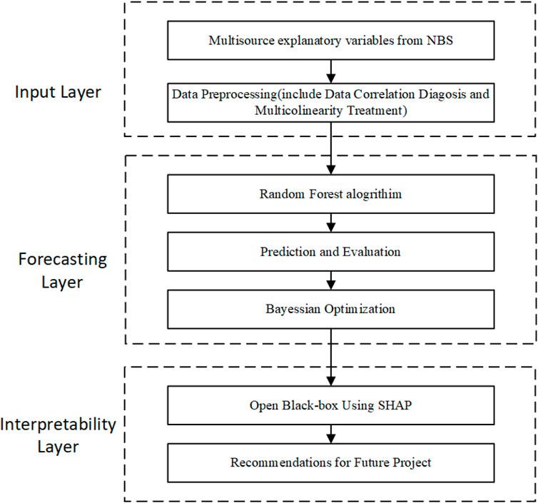
Figure 1. Methodological Framework for BO-RF-SHAP model.

3.1.1 Input layer

The first layer incorporates multisource explanatory variables obtained from the National Bureau of Statistics (NBS). To ensure data quality and consistency, categorical fields are transformed into numerical representations, and missing values are imputed using median replacement. Multicollinearity is addressed through Pearson’s correlation thresholding $|r|>$0.9, allowing the retention of a low-redundancy subset of driving factors. These preprocessing steps establish a robust foundation for subsequent modeling, ensuring that the feature set is both comprehensive and statistically reliable.

3.1.2 Forecasting layer

The second layer constitutes the predictive core of the framework. Within a five-fold cross-validation setting, the generalization performance of Random Forests (RF), Support Vector Regression (SVR), XGBoost, and GBDT is systematically compared to identify the most suitable baseline model. RF consistently demonstrates superior accuracy and robustness, motivating its selection as the primary predictive engine. To further enhance its performance, Bayesian Optimization (BO) is employed for automated hyperparameter tuning. By providing a principled global search strategy, BO efficiently determines the optimal hyperparameter configuration, denoted as ${\theta }^{*}$, thereby overcoming the inefficiency and suboptimality of manual trial-and-error approaches. The optimized model, referred to as BO-RF, generates air cargo demand forecasts with improved accuracy and stability. Formally, the predictive function can be expressed as Equation 1:

${\widehat{y}}_t=f_{\text{BO}-\text{RF}}\left(x_t\mid {\theta }^{*}\right),(1)$

Where ${\widehat{y}}_t$ denotes the predicted air cargo volume at time $t$, and$x_t=\left\{x_{1,t},x_{2,t}\dots ,x_{n,t}\right\}$ represents the feature vector of explanatory variables.

3.1.3 Interpretability layer

The third layer addresses the critical challenge of model transparency by grounding interpretability in cooperative game theory. Post-training, the BO-RF model is coupled with SHAP (SHapley Additive exPlanations), which adapts the Shapley value to feature attribution in predictive models. In this setting, each input variable is treated as a “player,” and its contribution to a given forecast is defined as the average marginal effect it produces when added to all possible coalitions of the remaining variables.

Operationally, SHAP yields local explanations (feature attributions for an individual forecast) and global explanations (aggregated patterns across all forecasts). Aggregating SHAP values across time reveals stable drivers and context-dependent effects, while SHAP interaction and dependence plots make nonlinear thresholds and cross-elasticities explicit. In this way, the SHAP layer not only quantifies which factors matter but also clarifies how they shape forecasts under different market conditions, thereby turning an accurate ensemble predictor into a transparent decision aid for logistics planning and transport policy.

Collectively, this three-tier design ensures that the proposed system is not only capable of generating accurate and robust forecasts, but also of producing theoretically grounded, decision-relevant explanations that enhance stakeholder confidence and support strategic decision-making in dynamic aviation markets.

3.2 Random forests: A nonlinear approach

Random Forest (RF) is an ensemble learning algorithm that constructs a multitude of decision trees and aggregates their outputs to achieve robust predictions. Each tree is trained on a bootstrap sample of the dataset, while random feature selection at each split introduces further diversity, reducing the risk of overfitting Liu and Mazumder [32]. This dual-randomization strategy enables RF to model complex, nonlinear dependencies between explanatory variables and the target. Unlike traditional linear models, which assume simple relationships between features, RF is capable of capturing intricate, nonlinear interactions due to its tree-based structure, where each decision tree splits the data recursively based on different feature combinations. This flexibility allows RF to detect patterns that may be missed by linear models, especially when features interact in complex, non-linear ways, as is often the case in transportation demand forecasting Barreñada et al. [33].

In regression tasks, the final prediction is obtained by averaging the outputs of all individual trees, which stabilizes forecasts and mitigates the variance inherent in single decision trees Probst and Boulesteix [34]. The model’s flexibility in handling high-dimensional data and heterogeneous predictors makes it particularly well-suited for forecasting tasks where multiple variables interact in complex ways. Moreover, RF offers a natural framework for feature importance analysis, which is further enhanced in this study through the use of game-theoretic SHAP values. SHAP values enable us to interpret the contributions of individual features in a nonlinear context, enhancing the transparency of the model and providing valuable insights for decision-making in aviation logistics.

3.3 Bayesian optimization for hyperparameter tuning

Bayesian Optimization (BO) offers a probabilistic and sample-efficient framework for global optimization, particularly suited to scenarios where the objective function is non-convex, computationally expensive, and analytically intractable Mustafa et al. [35]. In the context of air cargo volume forecasting, the objective is to identify the set of hyperparameters that minimize predictive error metrics such as the Root Mean Squared Error (RMSE) Garrido-Merchán [36]. Traditional tuning strategies, including grid search or random search, often require an excessive number of evaluations and risk converging to suboptimal configurations, especially when the feature space is high-dimensional and model training is computationally intensive. BO alleviates these limitations by leveraging uncertainty-aware modeling to systematically explore the hyperparameter space.

Formally, let the objective function be defined as Equation 2:

$f(\theta ): \mathrm{\Theta }\to \mathbb{R}(2)$

Where $\theta \in \mathrm{\Theta }$ denotes the hyperparameter configuration of the Random Forest (RF) model, and $f\left(\theta \right)$corresponds to the validation error (negative RMSE) derived from air cargo demand prediction. Because training and validating an RF on large-scale multisource datasets is computationally expensive, BO introduces a surrogate model—commonly a Gaussian Process (GP)—to approximate. $f\left(\theta \right)$

The GP surrogate, given historical evaluations ${{\mathcal{D}}_t=\left\{\left({\theta }_i,f\left({\theta }_i\right)\right)\right\}}_{i=1}^t$, provides a posterior distribution Equation 3:

$f(\theta )\mid {\mathcal{D}}_t\sim \mathcal{G}\mathcal{P}\left({\mu }_t(\theta ),k_t(\theta ,{\theta }^{\prime })\right)(3)$

where $u_t\left(\theta \right)$ is the posterior mean (expected predictive performance), and $k_t\left(\theta ,{\theta }^{\prime }\right)$ is the posterior covariance (epistemic uncertainty). By quantifying both the estimated outcome and the associated uncertainty, BO effectively identifies promising hyperparameter regions without resorting to exhaustive search.

The choice of the acquisition function plays a central role in guiding the optimization, including:

Expected Improvement (EI) Equation 4:

${\alpha }_{EI}(\theta )=\mathbb{E}\left[\max \left(0,f_{\text{best}}-f(\theta )\right){\mathcal{D}}_t\right](4)$

which favors regions with high potential to surpass the best observed performance, particularly important when marginal gains in forecasting accuracy can significantly affect logistics planning.

Upper Confidence Bound (UCB) Equation 5:

${\alpha }_{\mathit{UCB}}\left(\theta \right)={\mu }_t\left(\theta \right)+\kappa {\sigma }_t\left(\theta \right),(5)$

Where ${\sigma }_t\left(\theta \right)$ reflects uncertainty. In volatile contexts—such as cargo demand fluctuations driven by macroeconomic shocks—this formulation balances the exploitation of known effective hyperparameter regions with the exploration of under-sampled ones.

In the implementation of Bayesian Optimization within this study, the Expected Improvement (EI) acquisition function was selected as the primary strategy for guiding the search process. This choice is particularly appropriate given that the optimization objective is to minimize predictive errors, such as the Root Mean Squared Error (RMSE), in air cargo demand forecasting. By quantifying the expected gain over the current best solution, EI effectively aligns with the task of reducing forecast error while maintaining computational efficiency.

The iterative BO process is then defined as Equation 6:

${\theta }_{t+1}=\arg \underset{\theta \in \mathrm{\Theta }}{\max }\alpha (\theta ;{\mathcal{D}}_t),(6)$

with each new evaluation updating the GP posterior until convergence toward an optimal configuration ${\theta }^{*}$.

By systematically reducing the reliance on manual trial-and-error, BO enables the RF model to achieve superior configurations in fewer iterations. In practice, this efficiency is crucial for air cargo forecasting, where models must accommodate complex, nonlinear interactions among explanatory variables such as retail sales, trade volumes, and transport turnover. Moreover, the capacity to identify near-optimal solutions under computational constraints enhances both the robustness and the operational applicability of predictive systems in the aviation logistics sector.

3.4 SHAP explainability: a game-theoretic perspective

The interpretability of the proposed framework is grounded in the Shapley value, a concept originating from cooperative game theory. Formally, the Shapley value for a given feature i is expressed as Equation 7:

${\varphi }_i={\displaystyle \sum _{S\subseteq N\backslash \{i\}}}\frac{|S|!(n-|S|-1)!}{n!}\left[f(S\cup \{i\})-f(S)\right](7)$

where $N$ denotes the set of all features, $S$ is any subset excluding feature $i$, and $f(\cdot )$ represents the predictive function of the model. The term $f\left(S\cup \{i\}\right)-f\left(S\right)$ quantifies the marginal contribution of feature i when added to subset $S$, while the combinatorial coefficient ensures that the contributions are fairly averaged across all possible orderings of features. This formulation mirrors the principle of payoff allocation in cooperative games, where each player’s reward is determined by their average contribution across all coalitions. Translated into a machine learning context, features act as players and the model prediction serves as the collective payoff, thereby allowing the Shapley value to allocate the prediction outcome among features in a manner that is both rigorous and equitable.

Such an interpretation is particularly valuable in the case of air cargo demand forecasting, as it not only reveals which variables—such as waterborne freight, highway freight, or passenger traffic—drive model predictions, but also quantifies their relative importance in a game-theoretic sense. Consequently, the Shapley value provides a theoretically justified mechanism to bridge predictive accuracy with interpretability, ensuring that the model’s outputs can inform policy and operational decisions with transparency.

3.5 Evaluation metrics

To comprehensively assess the predictive performance of the models, several evaluation indicators are employed, including the coefficient of determination (R²), Mean Absolute Error (MAE), Root Mean Squared Error (RMSE) Wang et al. [37]. The R² value measures the proportion of variance in the dependent variable that is predictable from the independent variables, with higher values indicating stronger explanatory power of the model. RMSE quantifies the square root of the average squared differences between predicted and observed values, placing greater weight on larger deviations and thus highlighting prediction robustness. MAE, in contrast, provides the average magnitude of errors without considering their direction, offering a straightforward measure of predictive accuracy Qiu et al. [38]. In general, models with lower MAE and RMSE values and higher R² scores are considered to achieve superior predictive performance. The definitions of these statistical metrics are summarized as follows:

Root Mean Squared Error (RMSE) Equation 8:

$RMSE=\sqrt{\frac{1}{n}{\displaystyle \sum _{i=1}^n}{\left(\widehat{y_i}-y_i\right)}^2}(8)$

Mean Absolute Error (MAE) Equation 9:

$MAE=\frac{1}{n}{\displaystyle \sum _{i=1}^n}\left|\widehat{y_i}-y_i\right|(9)$

Coefficient of Determination (R²) Equation 10:

$R^2=1-\frac{{\sum }_{i=1}^n{\left(\widehat{y_i}-y_i\right)}^2}{{\sum }_{i=1}^n{\left(y_i-\bar{y}\right)}^2}(10)$

4 Data description

4.1 Data source

The empirical analysis in this study utilizes real-world monthly air cargo volume data from China Air Cargo Statistics, Civil Aviation Administration of China (CAAC) CAAC [39], covering the period from March 2006 to April 2025. This dataset contains aggregated freight throughput for major domestic and international routes, recorded in $10^5$ tons. To capture the multifactorial drivers of air cargo demand, additional explanatory variables were collected from authoritative sources, including National Bureau of Statistics of China (NBS) NBS [40] and General Administration of Customs of China GACC [41]. The final compiled dataset consists of 202 monthly observations (T = 202), with one target predictor (Air Cargo Volume) and 16 predictor variables aligned in the same time frequency as shown in Table 1.

Table 1

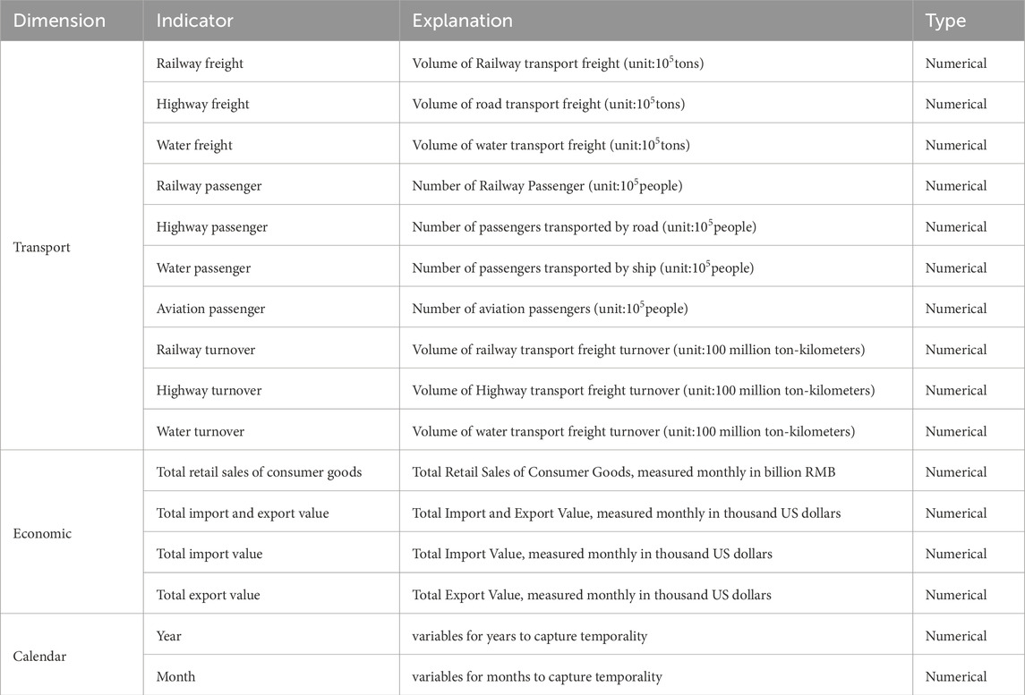
Table 1. Description of predictor variables in the dataset.

4.2 Data preprocessing

The preprocessing stage was designed to ensure data quality and statistical validity before model training. To mitigate the adverse influence of multicollinearity on model stability and predictive accuracy, this study first computed the Pearson correlation coefficient matrix for all candidate explanatory variables. The correlation matrix, as presented in Figure 2, provides a straightforward visualization of the linear interdependencies among transportation and macroeconomic indicators. To avoid redundancy caused by information overlap, the upper triangular portion of the matrix was systematically examined. Whenever a pair of variables exhibited a correlation coefficient with an absolute value exceeding the threshold of $|r|>$0.9, only the variable with the stronger association with the target variable (air cargo volume) was retained.

Figure 2

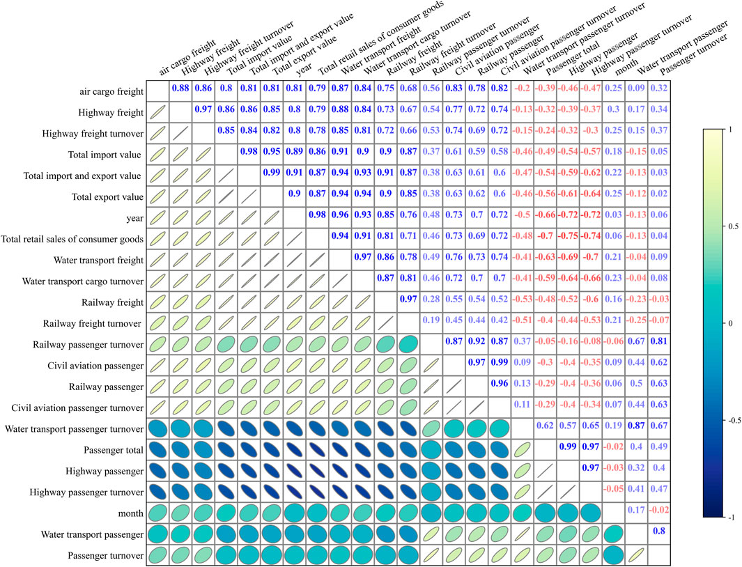
Figure 2. Pearson correlation plot.

The choice of a 0.9 threshold is consistent with established practices in empirical econometrics and machine learning, where correlation values above this level are generally considered to indicate near-collinearity, leading to unstable parameter estimation and inflated variance in predictive models. While lower thresholds (e.g., 0.7 or 0.8) are sometimes adopted, a stricter cut-off was selected in this study to minimize the risk of discarding potentially informative predictors, thereby striking a balance between dimensionality reduction and information preservation.

Through this filtering process, highly homogeneous indicators were removed. Representative examples include:

$•$ Highway freight volume and highway freight turnover $r\approx 0.98$;

$•$ Waterway freight volume and waterway freight turnover $r\approx 0.98$;

$•$ Total imports and exports versus exports/imports separately $r>0.98$;

$•$ Total passenger volume and highway passenger traffic $r\approx 0.99$.

As a result of this procedure, a parsimonious yet informative set of predictors was preserved. The retained features encompass both structural indicators, such as key freight, selected passenger turnover measures and temporal variables such as month, which capture seasonality, as presented in Figure 3. This refined set of variables not only reduces strong linear dependence among predictors but also enhances the interpretability of causal structures embedded in the data. Ultimately, this step improves the generalization capacity of the subsequent modeling framework by ensuring that the predictors contribute complementary, non-redundant information.

Figure 3

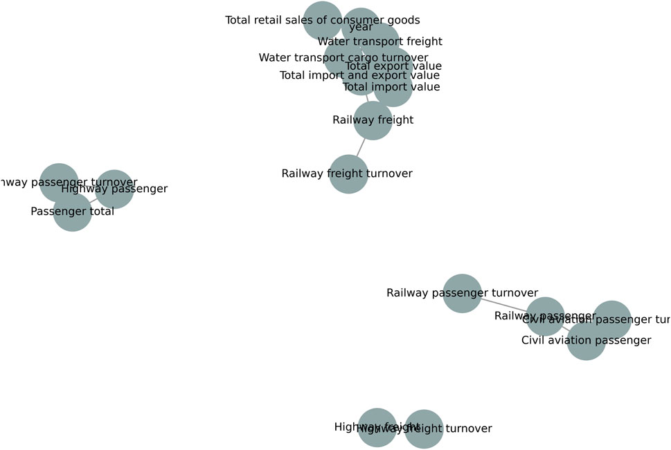
Figure 3. Correlation network plot.

5 Experiments and results

5.1 Model prediction comparison

To rigorously evaluate the predictive performance of different machine learning models, this study conducted a five-fold cross-validation (n splits = 5, shuffle = True, random state = 42) experiment on four representative algorithms: Random Forest (RF), Support Vector Regression (SVR), Extreme Gradient Boosting (XGBoost), and Gradient Boosted Decision Trees (GBDT). These models were selected due to their complementary methodological characteristics. RF is robust to noise and capable of capturing complex nonlinear relationships and high-order interactions; SVR serves as a classical kernel-based baseline with strong generalization in small-to-medium-sized datasets; XGBoost introduces advanced regularization and sparsity-aware mechanisms that enhance efficiency and predictive accuracy; GBDT represents the traditional gradient boosting framework widely adopted in regression tasks. The evaluation was performed using three standard metrics: Root Mean Squared Error (RMSE), Mean Absolute Error (MAE), and the coefficient of determination $R^2$. RMSE and MAE provide complementary perspectives on error magnitude, while $R^2$ assesses the proportion of variance in air cargo volume explained by the model.

The plots in Figure 4 demonstrate that the RF model achieves significantly better prediction performance compared to SVR, XGBoost and GBDT. Figure 4a highlights that the MAE for RF is the lowest at 3.54, compared to 5.22 for SVR, 4.17 for XGBoost and 4.01 for GBDT, indicating that RF predictions are much closer to the actual values. Similarly, Figure 4b shows that the RMSE for RF is 4.62, outperforming SVR (6.94), XGBoost (5.4) and GBDT (5.03), further affirming its superior predictive accuracy. The $R^2$ values in Figure 4c also reflect this trend, with RF achieving 0.8797, a notable improvement over SVR (0.7269), XGBoost (0.8351) and GBDT (0.8573), indicating RF’s higher ability to explain the variance in the data.

Figure 4

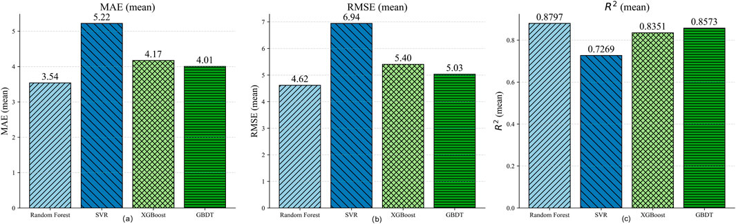
Figure 4. Performance comparison of RF, SVR, XGBoost and GBDT models: (a) MAE, (b) RMSE, (c) R.².

Based on these findings, RF was selected as the benchmark model for subsequent Bayesian optimization due to its superior balance of accuracy, robustness, and interpretability.

5.2 Bayesian optimization of random forest

Building on the superior baseline performance of the Random Forest (RF) model, Bayesian Optimization was employed to further enhance its predictive capability. The optimization process explored a hyperparameter search space defined as follows: number of estimators $n\underline{}estimators\in [\mathrm{10,300}]$, maximum tree depth $max\underline{}depth\in [\mathrm{3,15}]$, minimum samples required for node splitting $min\underline{}samples\underline{}split\in [\mathrm{2,10}]$, and minimum samples per leaf node $min\underline{}samples\underline{}leaf\in [\mathrm{1,10}]$. The optimization objective was set to the negative Root Mean Squared Error (–RMSE), and a five-fold cross-validation (n splits = 5, shuffle = True, random state = 42) was used to ensure robust performance assessment.

The prediction performance of the proposed model was evaluated after determining the optimal hyperparameters. The prediction results are presented in Figure 5, with the X and Y-axes representing the True and Predicted air cargo freight (10⁵ tons) respectively. The black dashed line indicates perfect prediction.

Figure 5

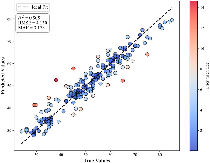
Figure 5. True values vs. predicted values of air cargo freight.

The optimized RF model achieved notable improvements in predictive accuracy. As shown in Figure 5, the cross-validation results indicate that the optimized RF attained an $R^2$ of approximately 0.905, an RMSE of 4.130, and an MAE of 3.178. The majority of predicted points are tightly clustered around the ideal fitting line, with residuals color levels concentrated in the lower range. This compact distribution indicates not only improved model fit but also enhanced robustness across varying sample ranges. Such stability is particularly critical in air cargo forecasting, where demand fluctuations and nonlinear relationships often challenge conventional predictive approaches.

The results demonstrate that Bayesian Optimization significantly strengthens RF’s predictive performance, yielding a model that is both accurate and reliable. Consequently, the optimized RF serves as the core forecasting framework for subsequent interpretability analyses based on SHAP.

5.3 Feature importance analysis with SHAP

5.3.1 Feature importance and directional effects

The SHAP summary plot provides a detailed interpretation of the relative importance and directional impact of the explanatory variables on air cargo freight prediction. As illustrated in Figure 6, Water transport freight and Highway freight emerge as the two most influential factors, with red points concentrated on the right-hand side of the x-axis and blue points on the left. This pattern indicates that higher volumes of waterborne and highway freight exert a strong positive contribution to air cargo, effectively driving the predicted values upward.

Figure 6

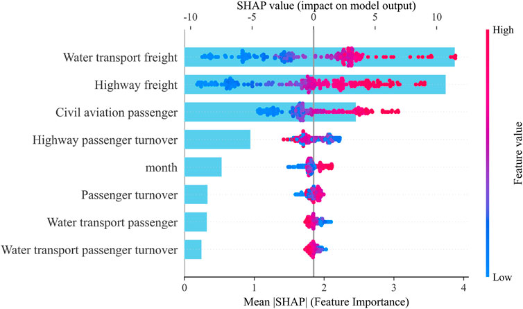
Figure 6. SHAP global explanation on RF model.

Civil aviation passenger volume also demonstrates a clear and consistent positive effect, reflecting that larger passenger flows are typically associated with higher air cargo demand. This result is consistent with the synergistic effect of bellyhold cargo capacity and enhanced route network density in civil aviation operations.

In contrast, Highway passenger turnover exhibits a more dispersed and symmetric distribution of SHAP values across both positive and negative regions, suggesting potential nonlinear or threshold effects (as further evidenced in Figure 7). The variable month shows a moderate level of influence, with red and blue points distributed closely around zero. This pattern reflects seasonal dynamics in air cargo demand, where peak travel periods boost freight volumes while off-peak months suppress them.

Figure 7

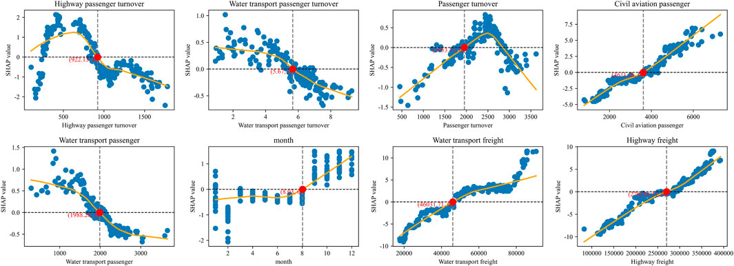
Figure 7. Univariate SHAP dependence plots illustrating trend and threshold.

Passenger turnover contributes positively overall, albeit with relatively smaller magnitude compared to freight-related indicators. Conversely, Water transport passenger volume and its associated turnover predominantly display negative SHAP values, indicating that higher levels of passenger water transport tend to reduce predicted air cargo volumes. This negative relationship is plausibly attributed to modal substitution or structural redistribution effects across transportation systems.

5.3.2 Univariate dependence analysis

To further probe into the nonlinear effects and threshold behaviors of individual predictors, SHAP dependence plots were constructed for the key explanatory variables in Figure 7. In each subplot, the x-axis represents the original feature value, while the y-axis denotes its corresponding SHAP value, reflecting the marginal contribution of the variable to the predicted air cargo volume. The smoothed orange curve highlights the overall trend, whereas the gray dashed line marks the zero baseline and critical turning points. The main findings are summarized as follows.

Highway passenger turnover exhibits an evident inverted U-shaped relationship. The SHAP value peaks positively around 900–1000, after which further increases in turnover reverse into negative contributions. This pattern suggests diminishing returns and possible congestion effects when highway passenger flows become excessive.

Water transport passenger turnover demonstrates a monotonic decline in SHAP values as turnover increases, crossing the zero threshold at approximately 5.5–6. This indicates that, at larger scales of waterway passenger activity, substitution effects emerge that suppress the demand for air freight.

Passenger turnover (total) also follows an inverted U-shaped curve, with an optimal positive contribution around 2000. Beyond this point, marginal effects turn negative, implying that overly intensive overall passenger movements reduce the incremental demand for air cargo.

Civil aviation passenger volume shows an approximately linear positive trend. The “zero impact point” occurs near 3600, beyond which larger passenger scales consistently elevate air freight volume.

Water transport passenger volume contributes monotonically negatively, crossing the zero axis around 1900–2000. This suggests that as waterway passenger flows grow, the stimulative effect on air freight weakens, consistent with substitution across transport modes.

Month reflects clear seasonal patterns. The SHAP curve turns positive after August, capturing the high-demand peak season that significantly raises air freight predictions, while earlier months mostly exert a suppressive effect.

Water transport freight exhibits a strong positive association, transitioning from negative to positive contributions around $4.6\times 10^4$. Higher levels of waterborne freight consistently amplify air cargo volume, highlighting complementarities in multimodal freight dynamics.

Highway freight displays an almost linear positive effect. Around $2.4\times 10^5$, the SHAP value approaches zero, and subsequent increases steadily lift predicted air cargo volume, underscoring its role as a major driver.

5.3.3 Bivariate dependence and interaction effects

To further explore the synergistic or substitutive relationships among explanatory variables, this study employed colored SHAP dependence plots that highlight the role of secondary features as shown in Figure 8. In each subplot, the x-axis denotes the raw value of the primary feature, the y-axis represents the corresponding SHAP value, while the color gradient of the scatter points reflects the magnitude of the secondary feature. A black smoothed line is fitted to reveal the overall interaction trend. This visualization enables the identification of interaction amplifications (synergy) and attenuation mechanisms (substitution), thereby enriching the interpretability of the prediction model.

Figure 8

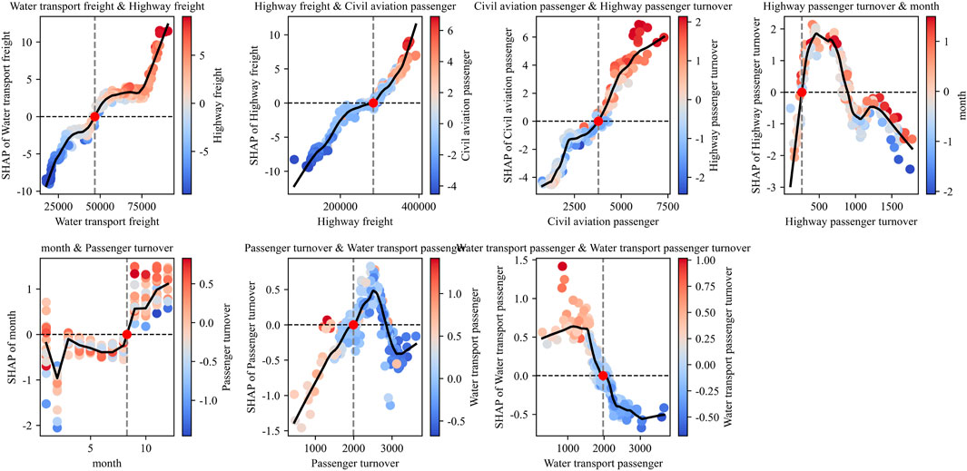
Figure 8. Bivariate SHAP dependence plots illustrating feature interactions.

Water transport freight $\times$ Highway freight (top-left): When both water transport freight and highway freight are simultaneously high (red dots), the SHAP values rise sharply, suggesting a strong supply-side resonance and synergistic amplification rather than simple substitution.

Highway freight $\times$ Civil aviation passenger: The slope of highway freight’s positive contribution becomes steeper as civil aviation passenger volume increases (red), indicating a reinforced human–cargo coupling effect.

Civil aviation passenger $\times$ Highway passenger turnover: Civil aviation passenger consistently pushes predictions upward, but when highway passenger turnover is high (red), the slope steepens further, reflecting that active passenger flows amplify the positive impact of civil aviation passenger volumes.

Highway passenger turnover $\times$ Month: At low-month phases (blue), highway passenger turnover shifts rapidly from negative to positive contributions; however, during peak-season months (red), excessive turnover levels turn negative, implying that seasonality modulates the threshold effect.

Month $\times$ Passenger turnover: In high-season months (red), passenger turnover strongly boosts the SHAP contribution of month, revealing a multiplicative effect of seasonal demand and travel intensity.

Passenger turnover $\times$ Water transport passenger: When water transport passenger levels are high (red), the positive contribution of passenger turnover diminishes, with its peak appearing earlier and at a lower magnitude, suggesting enhanced substitution effects between air and water passenger flows.

Water transport passenger $\times$ Water transport passenger turnover: When both features are high (red), the SHAP curve consistently trends downward, indicating a reinforced substitution mechanism within the water transport dimension, which suppresses air cargo demand.

Collectively, these bivariate dependence plots uncover nuanced interaction mechanisms: freight-related indicators exhibit strong synergy when co-elevated, while passenger-related indicators demonstrate both seasonal modulation and modal substitution. Such findings underscore the importance of capturing second-order interactions when designing predictive models for air cargo volume.

6 Conclusion and policy implications

6.1 Conclusion

This study advances the literature on air cargo forecasting by proposing an interpretable hybrid framework that combines Bayesian Optimization (BO), Random Forests (RF), and SHAP-based feature attribution derived from cooperative game theory. Drawing on a comprehensive dataset that integrates China’s air cargo statistics with macroeconomic indicators and multimodal transport variables, the model yields several key findings.

The empirical results underscore the superior predictive capability of the BO-RF framework. By consistently outperforming benchmark models such as SVM, XGBoost, and GBDT across RMSE, MAE, and R² metrics, the study demonstrates the value of BO in enhancing the robustness and accuracy of machine learning–based forecasting Xi et al. [42]. Beyond predictive performance, the integration of SHAP offers high interpretability, revealing that waterborne freight, highway freight, and civil aviation passenger volume emerge as the most influential predictors of cargo demand. These insights not only expose underlying demand dynamics but also form a practical foundation for aligning transport infrastructure investment and planning. Taken together, the combination of predictive accuracy and interpretability positions the proposed framework as a relevant tool for both short-term operational decision-making and longer-term strategic policy development in aviation logistics.

6.2 Policy implications

Enhance intermodal coordination and capacity alignment. The dominant SHAP contributions from highway and waterborne freight indicate that reinforcing multimodal links (e.g., port–airport–highway corridors) can raise transfer efficiency and stabilize air cargo throughput. Policymakers can use model outputs to prioritize corridor upgrades, cross-docking facilities, and time-window synchronization across modes.

Embed explainable AI in logistics governance. Regulators and logistics firms can adopt interpretable models such as BO–RF + SHAP to guide slot allocation, pricing adjustments, and compliance monitoring Tong et al. [43]. The transparency of SHAP values ensures that predictions are not only accurate but also trustworthy, supporting evidence-based policy implementation.

Guide long-horizon policy under uncertainty. By quantifying the influence of macroeconomic and transport variables, the framework equips policymakers and industry leaders with insights for resilient planning. It supports strategic initiatives such as capacity expansion, carbon reduction policies, and trade resilience strategies, ensuring aviation logistics adapts effectively to both structural changes and short-term shocks.

6.3 Future research directions

While the proposed framework provides both methodological innovation and practical value, its scope can be expanded in several promising directions. One avenue is the integration of real-time data sources, such as live shipping records, highway traffic flows, and customs clearance processes, to improve short-term responsiveness and forecasting accuracy. Another promising path involves hybrid deep learning extensions, in which BO-tuned Random Forests are combined with temporal architectures like LSTM or Transformer models to capture complex sequential dependencies Nunekpeku et al. [44]. Finally, game-theoretic simulation offers a fruitful opportunity, as SHAP-derived feature contributions could serve as inputs to model competitive and cooperative interactions among logistics stakeholders, enabling richer analyses of market dynamics and policy interventions.

Data availability statement

The original contributions presented in the study are included in the article/supplementary material, further inquiries can be directed to the corresponding author.

Author contributions

LZ: Conceptualization, Funding acquisition, Project administration, Validation, Visualization, Writing – original draft, Writing – review and editing. LJ: Data curation, Investigation, Methodology, Resources, Validation, Writing – review and editing.

Funding

The author(s) declare that financial support was received for the research and/or publication of this article. This research was funded by Jiangsu Provincial Higher Education Philosophy and Social Sciences Research Project grant number 2023SJYB2240 and supported by 2024 Jiangsu Province Higher Vocational Colleges Young Faculty Enterprise Practice Program fund NO.2024QYSJ122.

Conflict of interest

The authors declare that the research was conducted in the absence of any commercial or financial relationships that could be construed as a potential conflict of interest.

The reviewer D. H declared a shared affiliation with the author(s) to the handling editor at the time of review.

Generative AI statement

The author(s) declare that no Generative AI was used in the creation of this manuscript.

Any alternative text (alt text) provided alongside figures in this article has been generated by Frontiers with the support of artificial intelligence and reasonable efforts have been made to ensure accuracy, including review by the authors wherever possible. If you identify any issues, please contact us.

Publisher’s note

All claims expressed in this article are solely those of the authors and do not necessarily represent those of their affiliated organizations, or those of the publisher, the editors and the reviewers. Any product that may be evaluated in this article, or claim that may be made by its manufacturer, is not guaranteed or endorsed by the publisher.

References

1. İlgün Ayhan D, Alptekin SE. An integrated capacity allocation and dynamic pricing model designed for air cargo transportation. Appl Sci (2025) 15:5344. doi:10.3390/app15105344

CrossRef Full Text | Google Scholar

2. Nguyen QH. Modeling the volatility of international air freight: a case study of Singapore using the sarimax-egarch model. J Air Transport Management (2024) 117:102593. doi:10.1016/j.jairtraman.2024.102593

CrossRef Full Text | Google Scholar

3. Rodríguez Y, Olariaga OD. Air traffic demand forecasting with a bayesian structural time series approach. Periodica Polytechnica Transportation Eng (2024) 52:75–85. doi:10.3311/PPtr.20973

CrossRef Full Text | Google Scholar

4. Garg A, Shukla N, Wormer M (2024). Time series forecasting with high stakes: a field study of the air cargo industry. arXiv preprint arXiv:2407.

Google Scholar

5. Kosasih EE, Papadakis E, Baryannis G, Brintrup A. A review of explainable artificial intelligence in supply chain management using neurosymbolic approaches. Int J Prod Res (2024) 62:1510–40. doi:10.1080/00207543.2023.2281663

CrossRef Full Text | Google Scholar

6. Sahoo R, Pasayat AK, Bhowmick B, Fernandes K, Tiwari MK. A hybrid ensemble learning-based prediction model to minimise delay in air cargo transport using bagging and stacking. Int J Prod Res (2022) 60:644–60. doi:10.1080/00207543.2021.2013563

CrossRef Full Text | Google Scholar

7. Wu J, Chen X-Y, Zhang H, Xiong L-D, Lei H, Deng S-H. Hyperparameter optimization for machine learning models based on bayesian optimization. J Electron Sci Technology (2019) 17:26–40.

Google Scholar

8. Raiaan MAK, Sakib S, Fahad NM, Al Mamun A, Rahman MA, Shatabda S, et al. A systematic review of hyperparameter optimization techniques in convolutional neural networks. Decis Analytics J (2024) 11:100470. doi:10.1016/j.dajour.2024.100470

CrossRef Full Text | Google Scholar

9. Nasseri M, Falatouri T, Brandtner P, Darbanian F. Applying machine learning in retail demand prediction—a comparison of tree-based ensembles and long short-term memory-based deep learning. Appl Sci (2023) 13:11112. doi:10.3390/app131911112

CrossRef Full Text | Google Scholar

10. Abdulrashid I, Farahani RZ, Mammadov S, Khalafalla M, Chiang W-C. Explainable artificial intelligence in transport logistics: risk analysis for road accidents. Transportation Res E: Logistics Transportation Rev (2024) 186:103563. doi:10.1016/j.tre.2024.103563

CrossRef Full Text | Google Scholar

11. Thakur D, Biswas S. Permutation importance based modified guided regularized random forest in human activity recognition with smartphone. Eng Appl Artif Intelligence (2024) 129:107681. doi:10.1016/j.engappai.2023.107681

CrossRef Full Text | Google Scholar

12. Joy TT, Rana S, Gupta S, Venkatesh S. Fast hyperparameter tuning using bayesian optimization with directional derivatives. Knowledge-Based Syst (2020) 205:106247. doi:10.1016/j.knosys.2020.106247

CrossRef Full Text | Google Scholar

13. Yang C, Guan X, Xu Q, Xing W, Chen X, Chen J, et al. How can shap (shapley additive explanations) interpretations improve deep learning based urban cellular automata model? Comput Environ Urban Syst (2024) 111:102133. doi:10.1016/j.compenvurbsys.2024.102133

CrossRef Full Text | Google Scholar

14. Fatima SSW, Rahimi A. A review of time-series forecasting algorithms for industrial manufacturing systems. Machines (2024) 12:380. doi:10.3390/machines12060380

CrossRef Full Text | Google Scholar

15. Kontopoulou VI, Panagopoulos AD, Kakkos I, Matsopoulos GK. A review of arima vs. machine learning approaches for time series forecasting in data driven networks. Future Internet (2023) 15:255. doi:10.3390/fi15080255

CrossRef Full Text | Google Scholar

16. Ileri K. Comparative analysis of catboost, lightgbm, xgboost, rf, and dt methods optimised with pso to estimate the number of k-barriers for intrusion detection in wireless sensor networks. Int J Machine Learn Cybernetics (2025) 16:6937–56. doi:10.1007/s13042-025-02654-5

CrossRef Full Text | Google Scholar

17. Yu T, Zhu H (2020). Hyper-parameter optimization: a review of algorithms and applications. arXiv preprint arXiv:2003.05689.

Google Scholar

18. Pravin P, Tan JZM, Yap KS, Wu Z. Hyperparameter optimization strategies for machine learning-based stochastic energy efficient scheduling in cyber-physical production systems. Digital Chem Eng (2022) 4:100047. doi:10.1016/j.dche.2022.100047

CrossRef Full Text | Google Scholar

19. Rudin C. Stop explaining black box machine learning models for high stakes decisions and use interpretable models instead. Nat machine intelligence (2019) 1:206–15. doi:10.1038/s42256-019-0048-x

PubMed Abstract | CrossRef Full Text | Google Scholar

20. Hassija V, Chamola V, Mahapatra A, Singal A, Goel D, Huang K, et al. Interpreting black-box models: a review on explainable artificial intelligence. Cogn Comput (2024) 16:45–74. doi:10.1007/s12559-023-10179-8

CrossRef Full Text | Google Scholar

21. Ponce-Bobadilla AV, Schmitt V, Maier CS, Mensing S, Stodtmann S. Practical guide to shap analysis: explaining supervised machine learning model predictions in drug development. Clin translational Sci (2024) 17:e70056. doi:10.1111/cts.70056

PubMed Abstract | CrossRef Full Text | Google Scholar

22. Lundberg SM, Erion G, Chen H, DeGrave A, Prutkin JM, Nair B, et al. From local explanations to global understanding with explainable ai for trees. Nat machine intelligence (2020) 2:56–67. doi:10.1038/s42256-019-0138-9

PubMed Abstract | CrossRef Full Text | Google Scholar

23. Idrissi MI, Machado AF, Charpentier A (2025). Beyond shapley values: cooperative games for the interpretation of machine learning models. arXiv preprint arXiv:2506.

Google Scholar

24. Xu J, Chau H, Burden A (2025). From abstract to actionable: pairwise shapley values for explainable ai. arXiv preprint arXiv:2502.12525.

Google Scholar

25. Mohammadi M, Chau SL, Muandet K (2025). Computing exact shapley values in polynomial time for product-kernel methods. arXiv preprint arXiv:2505.

Google Scholar

26. Rozemberczki B, Watson L, Bayer P, Yang H-T, Kiss O, Nilsson S, et al. The shapley value in machine learning. In: The 31st international joint conference on artificial intelligence and the 25th European conference on artificial intelligence (2022). p. 5572–9.

Google Scholar

27. Li M, Sun H, Huang Y, Chen H. Shapley value: from cooperative game to explainable artificial intelligence. Autonomous Intell Syst (2024) 4:2. doi:10.1007/s43684-023-00060-8

CrossRef Full Text | Google Scholar

28. Ahmed KR, Ansari ME, Ahsan MN, Rohan A, Uddin MB, Rivin MAH, et al. Deep learning framework for interpretable supply chain forecasting using som ann and shap. Scientific Rep (2025) 15:26355. doi:10.1038/s41598-025-11510-z

PubMed Abstract | CrossRef Full Text | Google Scholar

29. Zhang R, Mao J, Wang H, Li B, Cheng X, Yang L. A survey on federated learning in intelligent transportation systems. IEEE Trans Intell Vehicles (2024) 10:3043–59. doi:10.1109/tiv.2024.3446319

CrossRef Full Text | Google Scholar

30. Białek J, Bujalski W, Wojdan K, Guzek M, Kurek T. Dataset level explanation of heat demand forecasting ann with shap. Energy (2022) 261:125075. doi:10.1016/j.energy.2022.125075

CrossRef Full Text | Google Scholar

31. Kahalimoghadam M, Thompson RG, Rajabifard A. An intelligent multi-agent system for last-mile logistics. Transportation Res Part E: Logistics Transportation Rev (2025) 200:104191. doi:10.1016/j.tre.2025.104191

CrossRef Full Text | Google Scholar

32. Liu B, Mazumder R. Randomization can reduce both bias and variance: a case study in random forests. J Machine Learn Res (2025) 26:1–49. doi:10.48550/arXiv.2402.12668

CrossRef Full Text | Google Scholar

33. Barreñada L, Dhiman P, Timmerman D, Boulesteix A-L, Van Calster B. Understanding overfitting in random forest for probability estimation: a visualization and simulation study. Diagn Prognostic Res (2024) 8:14. doi:10.1186/s41512-024-00177-1

PubMed Abstract | CrossRef Full Text | Google Scholar

34. Probst P, Boulesteix A-L. To tune or not to tune the number of trees in random forest. J Machine Learn Res (2018) 18:1–18. doi:10.48550/arXiv.1705.05654

CrossRef Full Text | Google Scholar

35. Mustafa A, Khattak KS, Khan ZH. Predicting short-term traffic with random forest: a granular data approach. In: International Conference on Energy, Power, Environment, Control and Computing (ICEPECC 2025); 19-20 February 2025; Hybrid Conference, Gujrat, Pakistan. Gujrat, Pakistan: IET (2025). 222–8.

CrossRef Full Text | Google Scholar

36. Garrido-Merchán EC (2025). Information-theoretic bayesian optimization: survey and tutorial. arXiv preprint arXiv:2502.06789.

Google Scholar

37. Wang H, Gu J, Wang M. A review on the application of computer vision and machine learning in the tea industry. Front Sustainable Food Syst (2023) 7:1172543. doi:10.3389/fsufs.2023.1172543

CrossRef Full Text | Google Scholar

38. Qiu D, Guo T, Yu S, Liu W, Li L, Sun Z, et al. Classification of apple color and deformity using machine vision combined with cnn. Agriculture (2024) 14:978. doi:10.3390/agriculture14070978

CrossRef Full Text | Google Scholar

39. CAAC (2025). Monthly transportation production statistics.

Google Scholar

40. NBS (2025). Monthly data statistics

Google Scholar

41. GACC (2025). Online customs statistics query platform.

Google Scholar

42. Xi Q, Chen Q, Ahmad W, Pan J, Zhao S, Xia Y, et al. Quantitative analysis and visualization of chemical compositions during shrimp flesh deterioration using hyperspectral imaging: a comparative study of machine learning and deep learning models. Food Chem (2025) 481:143997. doi:10.1016/j.foodchem.2025.143997

PubMed Abstract | CrossRef Full Text | Google Scholar

43. Tong Z, Zhang S, Yu J, Zhang X, Wang B, Zheng W. A hybrid prediction model for catboost tomato transpiration rate based on feature extraction. Agronomy (2023) 13:2371. doi:10.3390/agronomy13092371

CrossRef Full Text | Google Scholar

44. Nunekpeku X, Zhang W, Gao J, Adade SY-SS, Li H, Chen Q. Gel strength prediction in ultrasonicated chicken mince: fusing near-infrared and raman spectroscopy coupled with deep learning lstm algorithm. Food Control (2025) 168:110916. doi:10.1016/j.foodcont.2024.110916

CrossRef Full Text | Google Scholar