Airborne LIDAR system for real-time power lines recognition and terrain assessment

High speed flying drones and helicopters poses a significant flight safety risk due to the potential for collision with power lines and uneven landing grounds. There are few reports on light detection and ranging (LIDAR) systems for high-speed flight platforms. This study established an airborne, high-resolution light detection and ranging LIDAR system integrating a dual-wavelength laser source, a multi-beam transceiver scanning device, a two-dimensional mirror, and micro-electro-mechanical system (MEMS) scanning technology. Furthermore, the system achieves high-precision calibration with navigation systems by employing a voxel minimization strategy and a least squares fitting algorithm. It was compared with the performance of height-based clustering (k-means) and Hough transform and an improved point pillars convolutional neural network algorithm in power line recognition. The LIDAR system was tested on a high-speed helicopter platform reaching speeds of 120 km/h, enabling real-time recognition of power lines. Terrain assessment plays an important role in aircraft landing. The random sample consensus (RANSAC) method was used to extract ground points from the point cloud in real time at a rate of 5 ms per scan, ensuring terrain inclination estimation with minimal latency. This research provides an effective solution for real-time power line recognition and terrain assessment for flight platforms, thereby enhancing flight safety.

1 Introduction

LIDAR systems have emerged as a pivotal technique in the field of remote sensing applications, thanks to their high measurement accuracy, excellent pointing characteristics and ability to adapt to various platforms [1–4]. The advent of airborne LIDAR systems has significantly expanded the scope of LIDAR applications [5, 6]. Airborne LIDAR systems are currently widely used for advanced topographic mapping [7, 8], power line inspection [9–11], and navigation obstacle avoidance [12, 13].

For instance, Li et al. [14] designed lightweight, UAV-mounted LIDAR systems that are suitable for complex terrain conditions. They addressed system placement angle errors during imaging using a connection point-based self-calibration model and calibration scheme. This improved the accuracy of the system’s measurements and ultimately enabled the extraction of data on power lines 30 m away with a diameter of 4 cm. Kaputa et al. [15] designed the MX-1, a novel multimodal remote sensing airborne system. It is equipped with a high-precision global positioning system (GPS) and an inertial measurement unit (IMU). Mounted on the DJI Matrice 600 Pro UAV, the MX-1 can achieve an 18-min flight time with a spatial resolution of 1–3 cm RMS.

When using airborne LIDAR systems to identify power lines, it is crucial to process and analyses the acquired point cloud data efficiently. Jwa et al. [16] used an airborne LIDAR system to capture 30 points per square meter of the 3D power line scene and proposed a voxel-based line segment detector (VPLD) for the automatic reconstruction of 3D power line models. Guan et al. [17] proposed an LIDAR -supported detection concept for the intelligent, autonomous driving of UAVs. For the LiDAR data collected by UAV, intelligent optimization and risk prediction of the transmission line path are carried out through deep learning [18].

Airborne LIDAR systems also provide a useful tool for terrain assessment, where a key is to accurately extract ground points from the raw point cloud data. Filter-based extraction have been studied for decades and they are still the most widely used. Zhang et al. [19] introduced a progressive morphological filter to separate ground and non-ground points, which proved effective in forested areas. Sithole and Vosselman [20] conducted a comparative study of filtering techniques and highlighted the strengths of surface-based and TIN-based methods for complex urban terrain. Zhang et al. [21] developed the Cloth Simulation Filtering (CSF) method, which simulates a physical cloth draped over an inverted point cloud to identify ground points. This approach is widely praised for its simplicity, efficiency, and adaptability to rugged terrain. More recently, learning-based methods have been introduced for more refined extraction in varying data. Luo et al. [22] proposed a deep learning model that integrates local topological information with graph convolutional networks (GCNs) to enhance ground filtering from airborne LIDAR data in mountainous regions.

These limitations primarily manifest as an inability to adapt to high-speed flight platforms, as well as limited real-time processing and analysis of point cloud data. In order to overcome these challenges, this study proposes a settlement for airborne LIDAR systems. Based on the real-time processing of point clouds, the advantages of high-speed-borne LIDAR are revealed in terms of, e.g., calibration, power line recognition, slope gradient calculation, and digital terrain model (DTM) refinement.

2 System composition

2.1 System design

The airborne LIDAR system operates using a pulse-echo detection mechanism. It comprises a dual-wavelength laser source, dual detection units, transmission and reception optical components, a Position and Orientation System (POS), control and real-time processing units, and a Graphics Processing Unit (GPU) processing card. Vibration isolators are installed between the device and the installation reference to isolate the high-frequency vibrations of the airborne platform. Figure 1 illustrates the overall system design and vibration isolation features.

Figure 1

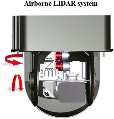
Figure 1. System design.

Taking into account the allocation of indices for each subsystem as shown in Table 1.

Table 1

Table 1. Design specifications.

2.2 Dual-wavelength laser

The key factors for improving the image quality of long-distance laser radar include the laser emission energy, repetition frequency, and angular resolution, etc. However, increasing the laser’s emission power by boosting its energy, can lead to a significant increase in its size and power consumption. This is particularly problematic in airborne platform applications, where space and power are highly constrained. Moreover, an excessively high repetition rate shortens the blur distance; This study proposes an innovative solution by designing and employing a high-repetition-rate fiber laser with dual wavelengths (1,064 nm and 1,550 nm). Each wavelength is equipped with two sets of lasers, with a 100 kHz repetition rate for each set, effectively balancing the relationship between size, power consumption, and performance.

To further enhance the accuracy and efficiency of measurements, this study also introduces a dual-channel receiving unit. These two receiving channels precisely isolate different wavelengths by using narrowband filters. With the design of this dual-wavelength laser, the data rate has been successfully increased to 400,000 measurement points per second, significantly enhancing the system’s real-time processing capabilities.

2.3 Opto-mechanical scanning mechanism

Under the requirements for long-range, wide-field and high-resolution scanning. Traditional mirrors are not suitable for this purpose. Although this technology provides a broad scanning range of over ±20°, its application in real-time imaging is limited by a scanning frequency below 300 Hz. Meanwhile, despite their somewhat limited scanning field, MEMS mirrors offer the possibility of super-resolution imaging thanks to their high scanning frequency exceeding 1 kHz and precise control capabilities.

In order to achieve long-range, wide-field and high-resolution scanning, this research project has designed a scanning system combining a two-dimensional scanning mirror (M1, M2) and a MEMS mirror. As illustrated in Figure 2, M1 scans in the X-axis direction and M2 in the Y-axis direction, together forming a two-dimensional scanning platform. The MEMS mirror then achieves super-resolution scanning in two dimensions, significantly improving imaging quality. Additionally, to cover a larger scanning area, the system is equipped with four sets of lasers (CoLID-I) and two sets of detectors, achieving efficient scanning of a large area through a compact transceiver common scanning mechanism. Figure 2A shows the schematic diagram of the system's scanning method. The receiving optics for the two bands adopt the same receiving optical system as shown in Figure 2B, thereby achieving the miniaturization of the entire machine.

Figure 2

Figure 2. (A) Schematic diagram of opt mechanical layout, (B) Receiving optical path diagram.

2.4 Processing unit

The processing circuit is implemented with a design based on Field-Programmable Gate Array (FPGA), Digital Signal Processor (DSP), and GPU, as shown in the schematic diagram and board card in Figure 3. Figure 3A shows the high-speed sampling processing board, while Figure 3B shows neural network processing board.

Figure 3

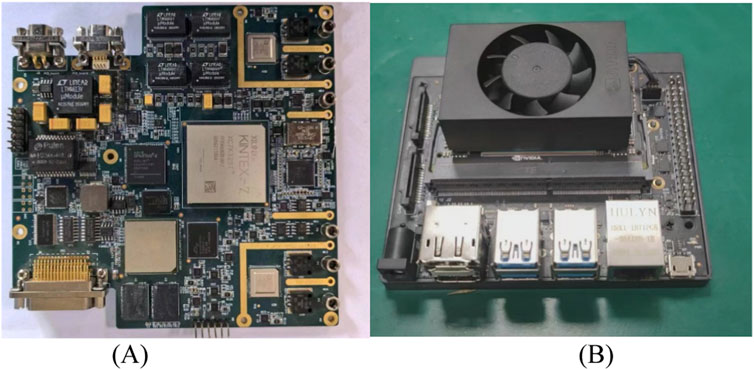
Figure 3. (A) High-Speed sampling processing board. (B) Neural network processing board.

2.5 POS system

During the high-speed motion and complex attitude variations of the airborne platform, including pitch, roll, and yaw, the LIDAR system often encounters distortion and layering issues in its point cloud data when performing scanning and imaging tasks. To effectively address this issue, this study integrates an advanced composite navigation system into the LIDAR system. This system is capable of capturing real-time positional and attitude information of the device, providing necessary corrections for the point cloud data during the dynamic imaging process. Specifically, the system incorporates a POS, which integrates two core components: the Global Navigation Satellite System (GNSS) and the IMU. The GNSS provides precise geographic location information, while the IMU can monitor and record the device’s attitude changes in real-time, including heading, pitch, and roll angles.

3 Methods

3.1 System calibration

This airborne LIDAR system is an assembly of laser scanning and composite navigation systems. Installation errors between these two systems (i.e., errors caused by misalignment of their coordinate systems in terms of position and axis parallelism) affect the absolute accuracy of the point cloud coordinates. This involves a calibration issue between the two systems. As a core component of multi-sensor fusion, the calibration model and the calibration scheme determine the precision of the final product.

A voxel (short for ‘volume pixel’) is the three-dimensional equivalent of a pixel in a two-dimensional image. Voxels effectively represent the spatial distribution of point clouds. If an object within the point cloud exhibits no layering or misalignment in three-dimensional space, the number of voxels it occupies should be minimized. This paper describes a high-precision calibration process for the LIDAR and composite navigation systems, combining voxel minimization with the least squares method.

The transformation Equation 1 from the LIDAR coordinate system $\left(X_b,Y_b,Z_b\right)$ to the inertial navigation coordinate system$\left(X_i,Y_i,Z_i\right)$ is as follows:

$\left[\begin{array}{c}{X}_i\\ Y_i\\ Z_i\end{array}\right]=C_b^i*\left(\left[\begin{array}{c}{X}_b\\ Y_b\\ Z_b\end{array}\right]-\left[\begin{array}{c}dx\\ dy\\ dz\end{array}\right]\right)(1)$

where $\left(dx,dy,dz\right)$ denotes the translational offset of the coordinate system origins along the axes, and $C_b^i$ is a function of the three installation angles (α, β, γ),representing the rotation matrix from the LIDAR coordinate system to the inertial navigation coordinate system.

The transformation Equation 2 from the inertial navigation coordinate system $\left(X_i,Y_i,Z_i\right)$ to the local horizontal geodetic coordinate system $\left(X_b,Y_b,Z_b\right)$ is as follows:

$\left[\begin{array}{c}{X}_g\\ Y_g\\ Z_g\end{array}\right]=C_i^g*\left[\begin{array}{c}{X}_i\\ Y_i\\ Z_i\end{array}\right](2)$

In the transformation matrix, $C_i^g$ is a function of the heading angle $\mathrm{{\rm A}}$, pitch angle P, and roll angle $R$. Representing the rotation matrix from the inertial navigation coordinate system to the local horizontal geodetic coordinate system.

The transformation Equation 3 from the local horizontal geodetic coordinate system $\left(X_g,Y_g,Z_g\right)$ to the Earth-Centered, Earth-Fixed (ECEF) coordinate system $\left(X_e,Y_e,Z_e\right)$ is as follows:

$\left[\begin{array}{c}{X}_e\\ Y_e\\ Z_e\end{array}\right]=C_g^e*\left[\begin{array}{c}{X}_e\\ Y_e\\ Z_e\end{array}\right]+\left[\begin{array}{c}{X}_0\\ Y_0\\ Z_0\end{array}\right](3)$

where $C_g^e$ represents the rotation matrix that transitions from the inertial navigation coordinate system to the local horizontal geodetic coordinate system, determined by the heading angle A, pitch angle P, and roll angle R. The transformation matrix $C_g^e$, which is a function of the geodetic latitude B0 and longitude L0, facilitates the rotation from the local horizontal geodetic coordinate system to the Earth-centered inertial (ECI) coordinate system. The coordinates $\left(X_0,Y_0,Z_0\right)$ correspond to the geocentric position of the device as determined by the composite navigation system.

In summary, The transformation relationship from the LIDAR coordinate system $\left(X_b,Y_b,Z_b\right)$ to the geocentric coordinate system $\left(X_e,Y_e,Z_e\right)$ is delineated as follows:

$\left[\begin{array}{c}{X}_e\\ Y_e\\ Z_e\end{array}\right]=C_g^e*C_i^g*C_b^i*\left(\left[\begin{array}{c}{X}_b\\ Y_b\\ Z_b\end{array}\right]-\left[\begin{array}{c}dx\\ dy\\ dz\end{array}\right]\right)+\left[\begin{array}{c}{X}_0\\ Y_0\\ Z_0\end{array}\right](4)$

where $C_g^e$, $C_i^g$, $X_0$, $Y_0$ and $Z_0$ can be derived from the positional and attitude data provided by the integrated navigation system. Meanwhile, $C_b^i$, dx, dy and dz are the calibration parameters required by the method described in this paper.

Specifically, we use Precise Point Positioning (PPP) with GPS to establish two high-precision ground control points. We then use a total station to extend these points to several others to form a high-precision control field (as illustrated in Figure 4). A laser scanner is used to single-point target the control points within the control field, recording the coordinates of each control point in the laser scanner frame $\left(X_b,Y_b,Z_b\right)$, and the positional and attitude information $\left(x,y,z,A,P,R\right)$ from the integrated navigation system at the time of targeting. At least six sets of data must be recorded. The recorded data are substituted into Equation 4, and the rotation matrix $C_b^i$ (which yields the three rotation parameters α, β, γ) and the three translation parameters $dx$, $dy$ and $dz$ are solved using the least squares method. Using these results as initial values, the dynamic point cloud data from the vehicle is transformed into the Earth-centered coordinate system. The point cloud is then voxelized, and the number of voxels is counted. Iterative adjustments are made to the rotation parameters α, β, γ and the translation parameters $dx$, $dy$ and $dz$. The iteration ranges for the angle parameters are ±2°, and for the distance parameters, they are ±20 cm, with iteration steps of 0.1° and 1 cm, respectively. If the number of voxels increases, iteration for the current parameter is stopped, and the next parameter is adjusted until all parameters have been refined (see algorithm flow in Figure 4). The six parameters at the end of the iteration process are the final calibration results. Figure 5A shows the ground calibration image. Figure 5B shows the ground calibration point cloud.

Figure 4

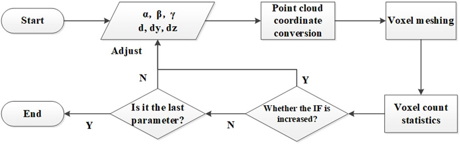
Figure 4. Calibration process flowchart.

Figure 5

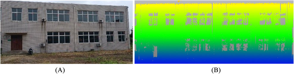
Figure 5. (A) Ground calibration image, (B) Ground calibration point cloud.

3.2 Principle of power line recognition

High-density airborne LIDAR point clouds contain power lines with distinct geometric priors: they usually appear as multiple parallel layers and can be approximated locally as straight or slightly curved lines. Based on these characteristics, this study proposes a power line extraction method using height-based clustering (k-means) and Hough transform line detection. Let the original point cloud be in Equation 5:

$\mathrm{{\rm P}}={\left\{p_i\right\}}^N,p_i={\left(x_i,y_i,z_i\right)}^T(5)$

Where N is the number of points, i is the different sequences, Since power lines typically exist within a certain height range, we define a height constraint in Equation 6:

$\left.P_s=\left.\left\{p_i\in P\right.\right|z_{\mathit{min}}<z_i<z_{\mathit{max}}\right\}(6)$

$P_s$ is thus obtained by filtering ground, tower, and noise points.

Power lines usually show layered distribution in the Z-axis direction. We apply k-means clustering to the height component $\left\{z_i\right\}$ in Equation 7:

$\underset{{\left\{H_j\right\}}_{j=1}^K}{\min }{\displaystyle \sum _{i=1}^{\left|P_s\right|}}\underset{1\le j\le K}{\min }{‖z_i-H_j‖}^2(7)$

K: expected number of layers (corresponding to power line levels), $H_j$: cluster center of the j-th layer.

Each candidate point is then assigned a cluster label as shown in Equation 8:

$o_i\in \left\{1,2,\dots ,K\right\},p_i\in P_s(8)$

Thus the candidate set is partitioned into sub-layer as shown in Equation 9.

$P_s={\mathrm{U}}_{j=1}^K{P}^{\left(j\right)},P^{\left(j\right)}=\left\{p_i|o_j=j\right\}(9)$

For each layer: $P^{\left(j\right)}$, the power lines are approximately linear in the X-Y plane, We first project the points in Equation 10:

$\mathrm{\Pi }:{\mathbb{R}}^3\to {\mathbb{R}}^2,\mathrm{\Pi }\left(x,y,z\right)=\left(x,y\right)(10)$

yielding in Equation 11:

${\mathcal{R}}^{\left(j\right)}=\left\{\left(x_i,y_i\right)|{p_i\in P}^{\left(j\right)}\right\}(11)$

A Hough transform is then applied for line detection. In polar coordinates, a line is represented as shown in Equation 12:

$\rho =\mathcal{x}\cos \theta +\mathcal{y}\sin \theta (12)$

Where $\mathcal{x},\mathcal{y}$ denote polar coordinate parameters, $\theta$ denote direction angle of the normal line of a straight line.

By searching for peaks in the accumulator space, we obtain a set of candidate lines as shown in Equation 13:

${\mathcal{L}}^{\left(j\right)}={\left\{\left({\rho }_k,{\theta }_k\right)\right\}}_{k=1}^{M_j}(13)$

For a candidate point: $p_i={\left(x_i,y_i,z_i\right)}^T$, the orthogonal distance to line $\left({\rho }_k,{\theta }_k\right)$ is shown in Equation 14:

$d_{ik}=\left|{\mathcal{x}}_i\cos {\theta }_k+{\mathcal{y}}_i\sin {\theta }_k-{\rho }_k\right|(14)$

Where $d_{ik}$ denote the vertical distance from the $i$ point to the $k$ candidate straight line, if the conditions specified in Equation 15 are met

$\underset{k}{\mathit{min}}{d}_{ik}<\delta (15)$

Where $\delta$ denote linear tolerance threshold. The point is classified as a power line point as shown in Equation 16:

$p_i\in P_{line}(16)$

The final set of power line is shown in Equation 17:

$P_{line}={\displaystyle \bigcup _{j=1}^K}{P_{line}}^{\left(j\right)}(17)$

3.3 Slope gradient calculation

Terrain assessment is an important application of aircraft landing at night. Robust identification of terrain characteristics improves segmentation accuracy and provides information about the monitoring area. In this study, we calculate the slope gradient to characterize the terrain of the landing area.

Firstly, we use the random sample consensus (RANSAC) method to extract ground points from the point cloud. RANSAC is a robust fitting approach designed to identify the best model parameters while rejecting outliers. Due to the noise and irregularities inherent in airborne LIDAR point clouds, RANSAC efficiently distinguishes ground points from non-ground objects, such as vegetation, infrastructure or measurement artefacts. RANSAC operates by iteratively selecting small subsets of points and estimating a plane model based on the selected samples. The core steps of the algorithm include random subset selection, model estimation, consensus evaluation and selection of the best model.

RANSAC identifies inlier points corresponding to the ground surface in a point cloud obtained through airborne LIDAR by iteratively selecting minimal subsets and fitting a plane model. The extracted ground points are then used to derive the Equation 18 of the best-fit plane.

$a\mathcal{x}+b\mathcal{y}+c\mathcal{z}+d=0(18)$

where a, b, c are the plane’s normal vector components, and d is the offset parameter.

Then, the slope gradient is determined by evaluating the deviation of the normal vector of the ground plane from the vertical axis. As the LIDAR system is calibrated, the obtained point cloud is regarded as horizontally referenced. Given a perfectly horizontal reference plane, the inclination angle $\theta$ of the extracted ground plane can be computed as shown in Equation 19:

$\theta =\mathit{arccos}\left(\frac{\left|\nu \right|}{\sqrt{a^2+b^2+{ac}^2}}\right)(19)$

where $\nu$ represents the vertical component of the normal vector.

The slope gradient metric effectively estimates terrain inclination, providing a simple yet robust mathematical representation of the ground surface. Integrating RANSAC with real-time airborne LIDAR processing enhances the reliability of terrain assessment, thereby improving the efficiency of power line detection systems.

3.4 Experiment

A flight test was conducted at a designated site to implement real-time power line detection and terrain assessment. A specific type of helicopter was used for the test, which took place in a forest area. The helicopter flew at an altitude of 200 m at a speed of 120 km/h, as shown in Figure 6.

Figure 6

Figure 6. Airborne platform experiment.

4 Applications and results

4.1 Calibration results

During the initial ground calibration stage, significant misalignment and layering phenomena were observed in the top-view point cloud data. Advanced calibration techniques were used to iteratively adjust the initial calibration parameters, which substantially improved the quality of the point cloud data. Figure 8 shows that the post-calibration point cloud of the building exhibits high alignment and consistency in the top-view projection. This improvement was further validated by conducting wall point cloud thickness measurements using Cloud Compare software, which increased precision from 0.14 m to 0.005 m, as shown in Figure 7 and in Figure 8. These results demonstrate the effectiveness of the calibration method in enhancing the accuracy of point cloud data.

Figure 7

Figure 7. Pre-calibration point cloud data.

Figure 8

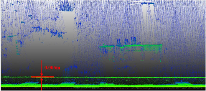
Figure 8. Post-calibration point cloud data.

4.2 Real-time power line recognition

This study combines LIDAR point cloud data and integrated navigation data in the field of power line detection. The point cloud coordinates are mapped to the geodetic coordinate system using transformation Equation 4. To minimize the amount of data while preserving the geometric integrity of the original point cloud, we use a uniform point cloud subsampling method. This method reduces data density while maintaining the original structure of the point cloud.

After subsampling, the average elevation of the point cloud is calculated. Points above this average are defined as non-ground points and are excluded, while those below are considered ground points. The eigenvalues for each point are computed and ranked in descending order, and the two largest are selected. The linearity of each point is then assessed by calculating the ratio of the difference between the largest and second-largest eigenvalues to the largest eigenvalue. Points exceeding a set threshold (0.79 in this study) are identified as power line points.

Elevation filtering algorithms were applied to the experimental data, achieving a detection rate of 90% original point cloud as depicted in Figure 9A. Figures 9B–E show the processing results. The detection of power lines exhibits outstanding performance not only in the side view but also maintains high accuracy in the top view. These results demonstrate that the method proposed in this study consistently achieves a high detection rate across different perspectives.

Figure 9

Figure 9. (A) Original point cloud (Red indicates power lines), (B) Z-X, (C) Z-Y, (D) X-Y, (E) Altitude distribution.

4.3 Point pillars recognition

In the field of deep learning-driven point cloud target detection, several algorithms such as PointNet [23], PointNet++ [24], Dynamic Graph Convolutional Neural Network (DGCNN) [25], Point RCNN [26], and KPConv [27] have demonstrated their strengths. However, the Point Pillars algorithm excels in balancing speed and accuracy. The algorithm innovatively converts complex 3D point cloud data into a 2D “pillar” representation, leveraging mature 2D Convolutional Neural Networks (2D CNNs) for efficient feature extraction and target detection. This approach significantly enhances computational efficiency while retaining the rich information of the point cloud data.

In order to meet the demand for the real-time, efficient detection of power lines from airborne platforms, this study employs an improved Point Pillars algorithm. In traditional vehicle-based target detection, the orientation of targets is usually defined by a single heading angle. However, for airborne platforms, precise target orientation requires consideration of three attitude angles. Consequently, critical modifications were made to the interface functions of the algorithm to enable it to adapt seamlessly from vehicle-based to airborne target detection scenarios. Furthermore, to enhance detection accuracy, the study integrates LIDAR point cloud data with POS measurements, converting the point cloud data into the geodetic coordinate system. This effectively mitigates deformation effects in Point Pillars projections caused by varying flight altitudes, as shown in Figure 10. By annotating and training on a large dataset (at least 6,000 frames), this study utilized SUSTech POINT software and the Open PCDet platform to train the point cloud data. The trained algorithm was then deployed on the NVIDIA Jetson NX platform for real-time power line detection on new point cloud data.

Figure 10

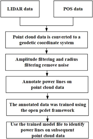
Figure 10. The point pillars algorithm process flowchart.

As illustrated in Figure 11, the Point Pillars algorithm, when deployed on the NVIDIA Jetson NX platform, accurately identified both power lines and towers, achieving an identification rate of 32% for individual power lines in 100 ms. Figure 11 corresponds to the same frame of data as Figure 9.

Figure 11

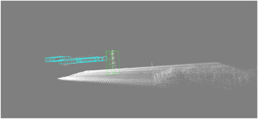
Figure 11. The point pillars algorithm identifies power lines and power towers. This diagram shows the effect of the algorithm. Blue represents power lines and green represents power towers. This frame of data includes 60,000 points, with 100 points for each individual power line.

The experimental results indicate that the combination of traditional elevation filtering algorithms and convolutional neural networks can effectively extract individual power lines from point cloud data. Due to the limited amount of pre training data, the correct recognition rate of neural networks is lower than that elevation algorithm.

4.4 Slope gradient calculation results

To validate the proposed method of calculating slope gradients, we performed slope gradient calculations using airborne LIDAR point cloud scans. We visualized the processed data, which included ground extraction and slope estimation, to assess the accuracy and efficiency of the algorithm.

Figure 12 shows the helicopter trajectory, the segmented ground and non-ground points, and the calculated slope gradient of the terrain. Please note that the slope gradient representing the ground was calculated dynamically in real time at a rate of 5 ms per point cloud scan, ensuring terrain inclination estimation with minimal latency. A comparison analysis was conducted between the measured data and the actual obtained slope data. The slope calculation error was 5%.

Figure 12

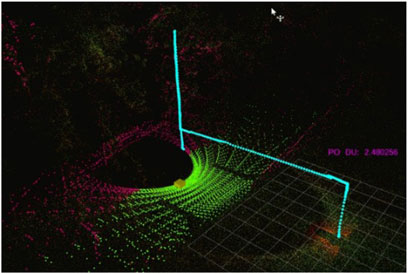
Figure 12. Slope gradient calculation in point cloud. Cyan represents the helicopter trajectory, green represents ground points, red represents non-ground points, the yellow box represents the helicopter landing position and the purple text shows the calculated slope gradient of the ground in real time.

This experimental visualization confirms the effectiveness of the proposed method for calculating slope gradients, which enables efficient and accurate terrain assessment for airborne LIDAR-based power line recognition systems.

5 Discussions and conclusion

This study involved the implementation of innovative design and implementation strategies to mitigate flight safety risks associated with night-time flying and landing, such as potential collisions with power lines and uneven landing grounds. The research successfully developed an efficient processing algorithm and platform, providing a robust technical foundation for the design of compact airborne LIDAR system. The system achieved long-distance, high-resolution detection capabilities and met critical real-time performance requirements. Regarding algorithm processing, the study successfully overcame the challenges of real-time coordinate transformation and power line detection and terrain assessment on a high-speed platform reaching speeds of 120 km/h.

As the pioneering study on high-speed flight platforms and LIDAR development, the promising gains may encourage other researchers to work on this topic. The merits of LiDAR are not limited to the aforementioned aspects. The system can be installed on top of any high-speed transport vehicle to form an safety monitoring system instantly. Additionally, the integration of infrared, camera and lidar data on the flight platform will be a important research focus in the future.

Data availability statement

The raw data supporting the conclusions of this article will be made available by the authors, without undue reservation.

Author contributions

CZ: Conceptualization, Validation, Project administration, Supervision, Methodology, Data curation, Writing – review and editing, Investigation, Writing – original draft, Funding acquisition, Visualization, Software, Resources, Formal Analysis. ML: Validation, Visualization, Writing – review and editing, Writing – original draft. DW: Methodology, Writing – review and editing, Writing – original draft, Visualization, Validation. FP: Resources, Writing – original draft, Data curation. HL: Writing – original draft, Formal Analysis, Conceptualization, Data curation, Investigation, Supervision, Methodology, Visualization. ZZ: Validation, Methodology, Conceptualization, Software, Writing – original draft, Resources, Funding acquisition, Visualization, Formal Analysis. YZ: Data curation, Writing – original draft, Validation, Resources, Visualization, Supervision, Methodology, Formal Analysis. JW: Visualization, Writing – original draft. JL: Visualization, Writing – original draft. PZ: Methodology, Writing – original draft, Visualization, Data curation. WH: Writing – original draft, Conceptualization.

Funding

The authors declare that no financial support was received for the research and/or publication of this article.

Conflict of interest

Authors CZ, FP, HL, and WH were employed by The 27th Research Institute of China Electronics Technology Group Corporation.

The remaining authors declare that the research was conducted in the absence of any commercial or financial relationships that could be construed as a potential conflict of interest.

Generative AI statement

The authors declare that no Generative AI was used in the creation of this manuscript.

Any alternative text (alt text) provided alongside figures in this article has been generated by Frontiers with the support of artificial intelligence and reasonable efforts have been made to ensure accuracy, including review by the authors wherever possible. If you identify any issues, please contact us.

Publisher’s note

All claims expressed in this article are solely those of the authors and do not necessarily represent those of their affiliated organizations, or those of the publisher, the editors and the reviewers. Any product that may be evaluated in this article, or claim that may be made by its manufacturer, is not guaranteed or endorsed by the publisher.

References

1. Pepe M, Fregonese L, Scaioni M. Planning airborne photogrammetry and remote-sensing missions with modern platforms and sensors. Eur J Remote Sensing (2018) 51(1):412–36. doi:10.1080/22797254.2018.1444945

CrossRef Full Text | Google Scholar

2. Zhang Z, Zhu L. A review on unmanned aerial vehicle remote sensing: platforms, sensors, data processing methods, and applications. Drones (2023) 7(6):398. doi:10.3390/drones7060398

CrossRef Full Text | Google Scholar

3. Midzak N, Yorks J, Zhang J, Limbacher J, Garay M, Kalashnikova O. Constrained retrievals of aerosol optical properties using combined lidar and imager measurements during the FIREX-AQ campaign. Front Remote Sensing (2022) 3:818605. doi:10.3389/frsen.2022.818605

CrossRef Full Text | Google Scholar

4. Li H, Xiang S, Zhang L, Zhu J, Wang S, Wang Y. A range ambiguity classification algorithm for automotive LiDAR based on FPGA platform acceleration. Front Phys (2023) 11:1290099. doi:10.3389/fphy.2023.1290099

CrossRef Full Text | Google Scholar

5. Browell EV, Grant WB, Ismail S. Airborne LIDAR systems. In: Laser remote sensing. CRC Press (2005). p. 741–98.

Google Scholar

6. Li X, Liu C, Wang Z, Xie X, Li D, Xu L. Airborne LIDAR: state-of-the-art of system design, technology and application. Meas Sci Technol (2020) 32(3):032002. doi:10.1088/1361-6501/abc867

CrossRef Full Text | Google Scholar

7. Tonina D, McKean JA, Benjankar RM, Wright CW, Goode JR, Chen Q, et al. Mapping river bathymetries: evaluating topobathymetric LIDAR survey. Earth Surf Process Landforms (2019) 44(2):507–20. doi:10.1002/esp.4513

CrossRef Full Text | Google Scholar

8. Höfle B, Rutzinger M. Topographic airborne LIDAR in geomorphology: a technological perspective. Z Geomorphologie-Supplementband (2011) 55(2):1–29. doi:10.1127/0372-8854/2011/0055s2-0043

CrossRef Full Text | Google Scholar

9. Azevedo F, Dias A, Almeida J, Oliveira A, Ferreira A, Santos T, et al. LIDAR-based real-time detection and modeling of power lines for unmanned aerial vehicles. Sensors (2019) 19(8):1812. doi:10.3390/s19081812

PubMed Abstract | CrossRef Full Text | Google Scholar

10. Yadav M, Chousalkar CG. Extraction of power lines using mobile LIDAR data of roadway environment. Remote Sensing Appl Soc Environ (2017) 8:258–65. doi:10.1016/j.rsase.2017.10.007

CrossRef Full Text | Google Scholar

11. Zhang N, Xu W, Dai Y, Ye C, Zhang X. Application of UAV oblique photography and LiDAR in power facility identification and modeling: a literature review. In: Third international conference on geographic information and remote sensing technology (GIRST 2024), 13551. SPIE (2025). p. 10–192. doi:10.1117/12.3059714

CrossRef Full Text | Google Scholar

12. Baras N, Nantzios G, Ziouzios D, Dasygenis M. Autonomous obstacle avoidance vehicle using LIDAR and an embedded system. In: 2019 8th international conference on modern circuits and systems technologies (MOCAST). IEEE (2019). p. 1–4.

CrossRef Full Text | Google Scholar

13. Hutabarat D, Rivai M, Purwanto D, Hutomo H. LIDAR-based obstacle avoidance for the autonomous mobile robot. In: 2019 12th international conference on information and communication technology and system (ICTS). IEEE (2019). p. 197–202.

Google Scholar

14. Li W, Tang L, Wu H. Development of mini UAV-borne LIDAR system and it’s application of power line inspection. Remote Sensing Technol Appl (2019) 34(2):269–74. doi:10.11873/j.issn.1004-0323.2019.2.0269

CrossRef Full Text | Google Scholar

15. Kaputa DS, Bauch T, Roberts C, McKeown D, Foote M, Salvaggio C. Mx-1: a new multi-modal remote sensing UAS payload with high accuracy GPS and IMU. In: 2019 IEEE systems and technologies for remote sensing applications through unmanned aerial systems (stratus). IEEE (2019). p. 1–4.

CrossRef Full Text | Google Scholar

16. Jwa Y, Sohn G, Kim HB. Automatic 3d powerline reconstruction using airborne LIDAR data. Int Arch Photogramm Remote Sens (2009) 38(Part 3):W8. doi:10.5194/isprsannals-I-3-167-2012

CrossRef Full Text | Google Scholar

17. Guan H, Sun X, Su Y, Hu T, Wang H, Wang H, et al. UAV-LIDAR aids automatic intelligent powerline inspection. Int J Electr Power Energ Syst (2021) 130:106987. doi:10.1016/j.ijepes.2021.106987

CrossRef Full Text | Google Scholar

18. Jin H, Wang Y, Zhou H, Li J. Monitoring data-driven optimization technology for overhead transmission line routing. In: 2025 4th international conference on energy, power and electrical technology (ICEPET). IEEE (2025). p. 537–42.

Google Scholar

19. Zhang K, Chen SC, Whitman D, Shyu ML, Yan J, Zhang C. A progressive morphological filter for removing nonground measurements from airborne LIDAR data. IEEE Transactions Geoscience Remote Sensing (2003) 41(4):872–82. doi:10.1109/TGRS.2003.810682

CrossRef Full Text | Google Scholar

20. Sithole G, Vosselman G. Experimental comparison of filter algorithms for bare-Earth extraction from airborne laser scanning point clouds. ISPRS J Photogrammetry Remote Sensing (2004) 59(1-2):85–101. doi:10.1016/j.isprsjprs.2004.05.004

CrossRef Full Text | Google Scholar

21. Zhang W, Qi J, Wan P, Wang H, Xie D, Wang X, et al. An easy-to-use airborne LiDAR data filtering method based on cloth simulation. Remote Sensing (2016) 8(6):501. doi:10.3390/rs8060501

CrossRef Full Text | Google Scholar

22. Luo Z, Zhang Z, Li W, Lin H, Chen Y, Wang C, et al. A local topological information aware based deep learning method for ground filtering from airborne Lidar data. In: 2021 IEEE international geoscience and remote sensing symposium IGARSS. IEEE (2021). p. 7728–31.

CrossRef Full Text | Google Scholar

23. Qi CR, Su H, Mo K, Guibas LJ. Pointnet: deep learning on point sets for 3d classification and segmentation. In: Proceedings of the IEEE conference on computer vision and pattern recognition (2017). p. 652–60.

Google Scholar

24. Qi CR, Yi L, Su H, Guibas LJ. Pointnet++: deep hierarchical feature learning on point sets in a metric space. Adv Neural Information Processing Systems (2017) 30. doi:10.48550/arXiv.1706.02413

CrossRef Full Text | Google Scholar

25. Wang Y, Sun Y, Liu Z, Sarma SE, Bronstein MM, Solomon JM. Dynamic graph cnn for learning on point clouds. ACM Trans Graphics (tog) (2019) 38(5):1–12. doi:10.1145/3326362

CrossRef Full Text | Google Scholar

26. Shi S, Wang X, Li H. Pointrcnn: 3D object proposal generation and detection from point cloud. In: Proceedings of the IEEE/CVF conference on computer vision and pattern recognition (2019). p. 770–9.

Google Scholar

27. Thomas H, Qi CR, Deschaud JE, Marcotegui B, Goulette F, Guibas LJ. Kpconv: flexible and deformable convolution for point clouds. In: Proceedings of the IEEE/CVF international conference on computer vision (2019). p. 6411–20.

Google Scholar