Invariant Subspace and Classification of Soliton Solutions of the Coupled Nonlinear Fokas-Liu System

1. Introduction

As vastly known, NPDEs are commonly applied to describe a lot of relevant dynamic processes and phenomena in mechanics, biology, physics, chemistry, etc. [1]. The solutions of NPDEs may provide a significant information for scientists and engineers. The ISM, proposed in Galaktionov [2] and modified in Ma [3], is one of strongest techniques to derive the solutions of NPDEs. The technique involve several invariant subspaces which are defined as subspaces of solutions to linear ODEs have been utilized to solve special NPDEs [3]. In Shen et al. [4], Zhu and Qu [5], and Song et al. [6], the maximal dimensions of invariant subspaces for studying n system of NPDEs has been reported. On the other hand, the ansatz technique is a powerful technique used in deriving the soliton solutions of NPDEs. The approach is based upon substituting an ansatz directly into the equation. The method has been used to obtain the solutions of several NPDEs [7–10]. In the last few decades, several powerful integration approaches have utilized to study many equations [11–19].

In this paper, we aim to study Equation (3) using the ISM [4–6]. Then, we will classify the soliton solutions of the equation by utilizing the the powerful ansatz approach [7, 8].

2. Model Description

Fokas and Liu [20] introduced a system of integrable KdV system. The system in it's original form is given by

$\begin{array}{ll}\{\begin{array}{c}{u}_t+{\upsilon }_x+(3{\beta }_1+2{\beta }_4){\beta }_{3}u{u}_x+(2+{\beta }_4{\beta }_1){\beta }_2{(u\upsilon )}_x\hfill \\ +{\beta }_1{\beta }_3\upsilon {\upsilon }_x+({\beta }_1+{\beta }_4){\beta }_2{u}_{xxx}+(1+{\beta }_4{\beta }_1){\beta }_2{\upsilon }_{xxx}=0,\hfill \\ \\ {\upsilon }_t+u_x+(2+3{\beta }_1{\beta }_4){\beta }_3\upsilon {\upsilon }_x+({\beta }_1+2{\beta }_4){\beta }_3{(u\upsilon )}_x\hfill \\ +{\beta }_1{\beta }_3{\beta }_{4}u{u}_x+({\beta }_1+{\beta }_4){\beta }_2{\beta }_4{u}_{xxx}+(1+{\beta }_1{\beta }_4){\beta }_2{\beta }_4{\upsilon }_{xxx}\hfill \\ =0.\hfill \end{array}\hfill & (1)\end{array}$

Gurses and Karasu [12] further simplified Equation (1) by considering a linear transformation of the form

$\begin{array}{ll}u=m_{1}r+n_{1}s,\upsilon =m_{2}r+n_{2}s,& (2)\end{array}$

where m₁, m₂, n₁ and n₂ are arbitrary constants, s and r new dynamical variables, qⁱ = (s, r). On properly choosing the constants, the coupled nonlinear Fokas-Liu system Equation (1) is reduced to a simpler form represented by:

$\begin{array}{ll}\{\begin{array}{c}{u}_t=au{u}_x+{(\upsilon u)}_x+b{\upsilon }_x,\hfill \\ {\upsilon }_t=c{u}_x+fu{u}_x+d{\upsilon }_x+3\upsilon {\upsilon }_x+e{\upsilon }_{xxx},\hfill \end{array}\hfill & (3)\end{array}$

with transformation parameters given by Baskonus et al. [15]:

$\begin{array}{l}{m}_2=\frac{{\beta }_1+{\beta }_4}{1+{\beta }_1{\beta }_4}{m}_1,n_2\frac{{\beta }_4{n}_1}{\delta {\beta }_3},\\ n_1=-\frac{1}{\delta {\beta }_3},\delta ={\beta }_1(1+{\beta }_4^2)+2{\beta }_4.& (4)\end{array}$

In Equation (3), u is the elevation of the water wave, υ is the surface velocity of water along x-direction [15]. The parameters a, b, c, e, f, d are constants. The only condition on the parameters a, b, c, e, f, d is given by c = fb. This guarantees the integrability of the above system.

3. The Invariant Subspace Method

Let us give a brief account of the ISM [6]

$\begin{array}{ll}\begin{array}{c}{\overline{u}}_t^1=F^1(x,{\overline{u}}^1,{\overline{u}}^2,\dots ,{\overline{u}}_{k_1}^1,{\overline{u}}_{k_1}^2),\\ {\overline{u}}_t^2=F^2(x,{\overline{u}}^1,{\overline{u}}^2,\dots ,{\overline{u}}_{k_2}^1,{\overline{u}}_{k_2}^2).\end{array}& (5)\end{array}$

The operator $F^1\equiv F^1\left[{\overline{u}}^1,{\overline{u}}^2\right]$ and $F^2\equiv F^1\left[{\overline{u}}^1,{\overline{u}}^2\right]$ are smooth functions with orders k₁ and k₂, namely

$\begin{array}{ll}\begin{array}{l}{\left(F_{{\overline{u}}_{k_1}^1}^1\right)}^2+{\left(F_{{\overline{u}}_{k_1}^2}^1\right)}^2\ne 0,{\left(F_{{\overline{u}}_{k_2}^1}^2\right)}^2+{\left(F_{{\overline{u}}_{k_2}^2}^2\right)}^2\ne 0.\hfill \end{array}& (6)\end{array}$

In the above and subsequent sections, we will apply the following notation

$\begin{array}{ll}{\overline{u}}_0^q={\overline{u}}^q(x,t),{\overline{u}}_j^q=\frac{\partial {\overline{u}}^q(x,t)}{\partial x^j},q=1,2;j=1,2,\dots & (7)\end{array}$

Let ${W}$ be a new linear subspace ${{W}}_{n_1}^1\times {{W}}_{n_2}^2,$ where

$\begin{array}{ll}{𝕎}_{n_q}^q={L}\{f_1{(x)}^q,\dots ,f_{n_q}{(x)}^q\}={\displaystyle \sum _{i=1}^{n_q}}{\lambda }_j^q{f}_j{(x)}^q,q=1,2& (8)\end{array}$

and $f_1{(x)}^q,\dots ,f_{n_q}{(x)}^q$ are linearly independent. If the vector operator F = (F¹, F²) satisfies the condition

$\begin{array}{ll}𝔽:{{W}}_{n_1}^1\times {{W}}_{n_2}^2\to {{W}}_{n_1}^1\times {{W}}_{n_2}^2,& (9)\end{array}$

i.e.,

$\begin{array}{ll}{F}^q:{{W}}_{n_1}^1\times {{W}}_{n_2}^2\to {{W}}_{n_q}^q,q=1,2& (10)\end{array}$

satisfies

$\begin{array}{l}{F}^q[{\displaystyle \sum _{j=1}^{n_1}}{\lambda }_j^1{f}_j^1(x),{\displaystyle \sum _{j=1}^{n_2}}{\lambda }_j^2{f}_j{(x)}^2]\\ ={\displaystyle \sum _{j=1}^{n_q}}{\psi }_j^q({\lambda }_1^1,\dots ,{\lambda }_{n_1}^1,{\lambda }_1^2,\dots ,{\lambda }_{n_2}^2)f_j^q(x).& (11)\end{array}$

Then the vector operator 𝔽 admit an invariant subspace given by ${W}$. If the subspace ${W}$ is being admitted by the operator 𝔽, then Equation (5) has a solution given by

$\begin{array}{ll}{\overline{u}}^q={\displaystyle \sum _{j=1}^{n_q}}{\lambda }_j^q(t)f_j{(x)}^q,q=1,2,& (12)\end{array}$

with ${\lambda }_j^q(t)$ being functions of t satisfying the following ODEs

$\begin{array}{ll}\frac{d{\lambda }_j^q(t)}{dt}={\psi }_j^q({\lambda }_1^1(t),\dots ,{\lambda }_{n_1}^1(t),{\lambda }_1^2(t),\dots ,{\lambda }_{n_2}^2(t))q=1,2.& (13)\end{array}$

Suppose ${{W}}_{n_q}^q={L}\{f_1^q(x),\dots ,f_{n_q}^q(x)\}$ is generated by the solutions of the linear n_qth-order ODEs

$\begin{array}{l}{{L}}^q\left[y\right]=y_q^{(n_q)}+a_{n_q-1}^q(x)y^{(n_q-1)}+\cdots \\ +a_1^q(x)y_q^{\prime }+a_0^q(x)y_q=0,q=1,2.& (14)\end{array}$

Thus, the invariant conditions represented by

$\begin{array}{ll}{{L}}^q[F^q[{\overline{u}}^1,{\overline{u}}^2]]{|}_{[H_1]\cap [H_2]}=0,q=1,2& (15)\end{array}$

one can denote by [H_q] the equation ${{L}}^q\left[{\overline{u}}^q\right]=0$ and its differentials w.r.t x. Once one determined the maximal dimension, then the complete classification and exact solutions of the equation can be investigated. From Equation (15) representing the invariant condition, the estimation has been determined in Shen et al. [4].

Theorem 3.1. Let 𝔽 = (F¹, F²) be a nonlinear vector and be coupled. We can assume without loss of generality (k₁ ≥ k₂). If the operator 𝔽 admits the invariant subspace ${{W}}_{n_1}^1\times {{W}}_{n_2}^2(n_1\ge n_2>0),$ then there holds n₁ − n₂ ≤ k₂, n₁ ≤ 2(k₁ + k₂) + 1.

In theorem 2.1, the operator 𝔽 is couple meaning

$\begin{array}{l}{\left(F_{{\overline{u}}_0^2}^1\right)}^2+{\left(F_{{\overline{u}}_1^2}^1\right)}^2+\cdots +{\left(F_{{\overline{u}}_{k_1}^2}^1\right)}^2\ne 0\hfill \\ {\left(F_{{\overline{u}}_0^2}^2\right)}^2+{\left(F_{{\overline{u}}_1^2}^2\right)}^2+\cdots +{\left(F_{{\overline{u}}_{k_1}^2}^2\right)}^2\ne 0.\hfill & (16)\end{array}$

𝔽 represents a nonlinear vector, i.e., for certain i₀, j₀, l₀ ∈ {1, 2}, p₀, q₀ ∈ {0, 1, …, k_i0}, there holds

$\begin{array}{ll}\frac{\partial F^{i_0}}{\partial {\overline{u}}_{p_0}^{j_0}\partial {\overline{u}}_{q_0}^{l_0}}\ne 0.& (17)\end{array}$

In the case of k₁ = k₂, the estimation of maximal dimension is given in Zhu and Qu [5]. Next, we consider the case 0 < n₁ < n₂. We give the following results from Song et al. [6] in a more general form which we shall apply in the next section.

4. Application to the Coupled Nonlinear Fokas-Liu System

In this section, we will construct the invariant subspace and solutions of Equation (3). Let us take an invariant subspace ${{W}}_{2,2}={{W}}_2^1\times {{W}}_2^2$ defined by

$\begin{array}{ll}\begin{array}{c}{{L}}^1\left[y_1\right]=y_1^{{}^{″}}+a_1{y}_1^{{}^{\prime }}+a_0{y}_1=0,\\ {{L}}^2\left[y_2\right]=y_2^{{}^{″}}+b_1{y}_2^{{}^{\prime }}+b_0{y}_2=0.\end{array}& (18)\end{array}$

where a₀, a₁, b₀, and b₁ are constants to be determined. The corresponding invariance conditions are given by

$\begin{array}{ll}\begin{array}{c}(D^{2}F+a_{1}DF+a_{0}F){|}_{u\in {{W}}_2^1,v\in {{W}}_2^2}=0,\\ (D^{2}G+b_{1}DG+b_{0}G){|}_{u\in {{W}}_2^1,v\in {{W}}_2^2}=0,\end{array}& (19)\end{array}$

where

$\begin{array}{ll}\{\begin{array}{c}{u}_t=F=au{u}_x+{(\upsilon u)}_x+b{\upsilon }_x,\hfill \\ {\upsilon }_t=G=c{u}_x+fu{u}_x+d{\upsilon }_x+3\upsilon {\upsilon }_x+e{\upsilon }_{xxx}.\hfill \end{array}\hfill & (20)\end{array}$

Substitute the expressions for F and G into the above equations, we obtain an overdetermined system of algebraic expressions which can be solved in general to obtain the invariant conditions given by

$\begin{array}{ll}{a}_0=0,a_1=0,b_0=0,b_1=0,b=b,c=c,f=f.& (21)\end{array}$

Therefore, Equation (14) reduces to

$\begin{array}{ll}\begin{array}{c}{{L}}^1\left[y_1\right]=y_1^{{}^{″}}=0,\\ {{L}}^2\left[y_2\right]=y_2^{{}^{″}}=0.\end{array}& (22)\end{array}$

Thus, we get ${{W}}_2^1=span\left\{1,x\right\}$ and ${{W}}_2^2=span\left\{1,x\right\}.$ This invariant subspace takes the exact solution of Equation (3) as

$\begin{array}{ll}\begin{array}{c}u(x,t)={\lambda }_3(t)+x{\lambda }_4(t),\\ \upsilon (x,t)={\lambda }_1(t)+x{\lambda }_2(t).\end{array}& (23)\end{array}$

where λ_i(t), i = 1, 2, 3 are unknown function to be determined. Putting Equation (23) into Equation (3), we acquire the following system of ODEs:

$\begin{array}{ll}\{\begin{array}{c}-2{\lambda }_3(t){\lambda }_1(t)+{\lambda }_3^{{}^{\prime }}(t)=0,\hfill \\ -{\lambda }_3{(t)}^{2}f-3{\lambda }_1{(t)}^2+{\lambda }_1^{{}^{\prime }}(t)=0,\hfill \\ -{\lambda }_4(t){\lambda }_1(t)-{\lambda }_3(t){\lambda }_2(t)-a{\lambda }_3(t)-b{\lambda }_1(t)+{\lambda }_4^{{}^{\prime }}(t)=0,\hfill \\ -{\lambda }_4(t){\lambda }_3(t)f-c{\lambda }_3(t)-3{\lambda }_1(t){\lambda }_2(t)-d{\lambda }_1(t)+{\lambda }_2^{{}^{\prime }}(t)=0.\hfill \end{array}\hfill & (24)\end{array}$

Solving Equation (24), we acquire

$\begin{array}{l}{\lambda }_1(t)=\frac{-1}{3t+c_3},\\ {\lambda }_2(t)=\frac{-d(-3t+c_3)+3c_2}{-3t+c+3},\\ {\lambda }_3(t)=0,\\ {\lambda }_4(t)=-b+\frac{c_1}{{(-3t+c_3)}^{\frac{1}{3}}}.& (25)\end{array}$

Subsequently, we obtain the following algebraic function solution

$\begin{array}{l}u(x,t)=-bx+\frac{x{c}_1}{{(-3t+c_3)}^{\frac{1}{3}}},\\ \upsilon (x,t)=\frac{-1}{3t+c_3}+\frac{x(-d(-3t+c_3)+3c_2)}{-3t+c_3}.& (26)\end{array}$

where c_i(i = 1, …, 3) are arbitrary constants.

5. Ansatz Approach

In this section, we will utilize the ansatz approach to derive the topological, non-topological and singular soliton solutions of Equation (3).

5.1. Non Topological Solitons

The non topological soliton solution of Equation (3) can be represented by the following ansatz:

$\begin{array}{ll}u(x,t)={\sigma }_1{\mathrm{\text{sech}}}^{p_1}\tau ,v(x,t)={\sigma }_2{\mathrm{\text{sech}}}^{p_2}\tau ,& (27)\end{array}$

where τ = η(x − vt), σ₁, σ₂, p₁ and p₂ are to be determined later. η is the wave number of the soliton. Putting Equation (27) into Equation (3), we obtain

$\begin{array}{ll}\{\begin{array}{l}v\eta {\text{sech}}^{1+p_1}(\tau )\sinh (\tau )p_1{\rho }_1+a\eta {\text{sech}}^{1+2p_1}(\tau ){\sinh }_1^p(\tau ){\rho }_1^2+\hfill \\ b\eta {\text{sech}}^{1+p_2}(\tau )\sinh (\tau )p_2{\rho }_2+\eta {\text{sech}}^{1+p_1+p_2}(\tau )\sinh (\tau )p_1{\rho }_1{\rho }_2+\hfill \\ \eta {\text{sech}}^{1+p_1+p_2}(\tau )\sinh (\tau )p_2{\rho }_1{\rho }_2=0,\hfill \\ \hfill \\ c\eta {\text{sech}}^{1+p_1}(\tau )\sinh (\tau )p_1{\rho }_1+f\eta {\text{sech}}^{1+2p_1}(\tau )\sinh (\tau )p_1{\rho }_1^2+\hfill \\ d\eta {\text{sech}}^{1+p_2}(\tau )\sinh (\tau )p_2{\rho }_2+v\eta \text{sech}{)}^{1+p_2}(\tau )\sinh (\tau )p_2{\rho }_2-\hfill \\ 2e{\eta }^3{\text{sech}}^{1+p_2}(\tau )\sinh (\tau )p_2{\rho }_2+2e{\eta }^3{\text{sech}}^{3+p_2}(\tau )\sinh {(\tau )}^3{p}_2{\rho }_2-\hfill \\ 3e{\eta }^3{\text{sech}}^{1+p_2}(\tau )\sinh (\tau )p_2^2{\rho }_2+3e{\eta }^3{\text{sech}}^{3+p_2}(\tau )\sinh {(\tau )}^3{p}_2^2{\rho }_2+\hfill \\ e{\eta }^3{\text{sech}}^{3+p_2}(\tau )\sinh {(\tau )}^3{p}_2^3{\rho }_2+3\eta {\text{sech}}^{1+2p_2}(\tau )\sinh (\tau )p_2{\rho }_2^2\hfill \\ =0.\hfill \end{array}& (28)\end{array}$

Upon equating the exponents in p₁ and p₂, we acquire

$\begin{array}{ll}3+p_2=1+p_1+p_2,& (29)\end{array}$

$\begin{array}{ll}3+p_2=1+2p_2,& (30)\end{array}$

thus, we obtain p₁ = p₂ = 2. Putting into Equation (28), we acquire

$\begin{array}{ll}\{\begin{array}{c}2v\eta \mathrm{\text{sech}}{(\tau )}^2{\rho }_{1}tanh(\tau )+2a\eta {\mathrm{\text{sech}}}^4(\tau ){\rho }_1^{2}tanh(\tau )+\hfill \\ 2b\eta {\mathrm{\text{sech}}}^2(\tau ){\rho }_{2}tanh(\tau )+4\eta {\mathrm{\text{sech}}}^4(\tau ){\rho }_1{\rho }_{2}tanh(\tau )=0,\hfill \\ \\ 2c\eta {\mathrm{\text{sech}}}^2(\tau ){\rho }_{1}tanh(\tau )+2f\eta {\mathrm{\text{sech}}}^4(\tau ){\rho }_1^{2}tanh(\tau )+\hfill \\ 2d\eta {\mathrm{\text{sech}}}^2(\tau ){\rho }_{2}tanh(\tau )+2v\eta {\mathrm{\text{sech}}}^2(\tau ){\rho }_{2}tanh(\tau )+\hfill \\ 8e{\eta }^3{\mathrm{\text{sech}}}^2(\tau ){\rho }_{2}tanh(\tau )-24e{\eta }^3{\mathrm{\text{sech}}}^4(\tau ){\rho }_{2}tanh(\tau )+\hfill \\ 6\eta {\mathrm{\text{sech}}}^4(\tau ){\rho }_2^{2}tanh(\tau )=0.\hfill \end{array}\hfill & (31)\end{array}$

After making some algebraic computations, we obtain the following soliton parameters:

$\begin{array}{l}v=\frac{ab}{2},\eta =\frac{1}{2}\sqrt{\frac{-a^{2}b+4c-2ad}{2ae}},\\ {\rho }_1=\frac{3(a^{2}b-4c+2ad)}{3a^2+4f},{\rho }_2=-\frac{a{\rho }_1}{2}.& (32)\end{array}$

The non-topological soliton solutions of Equation (3) are given by

$\begin{array}{ll}\{\begin{array}{c}u(x,t)=\frac{3(a^{2}b-4c+2ad)}{3a^2+4f}{\mathrm{\text{sech}}}^2\left[\frac{1}{2}\sqrt{\frac{-a^{2}b+4c-2ad}{2ae}}(-\frac{1}{2}abt+x)\right],\hfill \\ v(x,t)=-\frac{3a(a^{2}b-4c+2ad)}{2(3a^2+4f)}{\mathrm{\text{sech}}}^2\left[\frac{1}{2}\sqrt{\frac{-a^{2}b+4c-2a}{2ea}}(-\frac{1}{2}abt+x)\right].\hfill \end{array}\hfill & (33)\end{array}$

5.2. Topological Solitons

The non topological soliton solution of Equation (3) can be represented by the following ansatz:

$\begin{array}{ll}u(x,t)={\sigma }_1{\mathrm{\text{tanh}}}^{p_1}\tau ,v(x,t)={\sigma }_2{\mathrm{\text{tanh}}}^{p_2}\tau ,\hfill & (34)\end{array}$

where τ = η(x − vt). Putting Equation (34) into Equation (3), we obtain

$\begin{array}{ll}\{\begin{array}{l}-v\eta \text{csch}(\tau ){\text{sech}}^{p_1}(\tau ){\rho }_1\tanh {(\tau )}^{p_1}-a\eta \text{csch}(\tau )\text{sech}(\tau )p_1{\rho }_1^2{\tanh }^{2p_1}(\tau )-\hfill \\ b\eta \text{csch}(\tau ){\text{sech}}^{p_2}(\tau ){\rho }_2{\tanh }^{p_2}(\tau )-\eta \text{csch}(\tau ){\text{sech}}^{p_1}(\tau ){\rho }_1{\rho }_2{\tanh }^{p_1+p_2}(\tau )-\hfill \\ \eta \text{csch}(\tau )\text{sech}(\tau )p_2{\rho }_1{\rho }_2\tanh {)}^{p_1+p_2}(\tau )=0,\hfill \\ \hfill \\ -c\eta \text{csch}(\tau )\text{sech}(\tau )p_1{\rho }_1{\tanh }^{p_1}(\tau )-f\eta \text{csch}(\tau )\text{sech}(\tau )p_1{\rho }_1^2{\tanh }^{2p_1}(\tau )-\hfill \\ d\eta \text{csch}(\tau )\text{sech}(\tau )p_2{\rho }_2{\tanh }^{p_2}(\tau )-v\eta \text{csch}(\tau )\text{sech}(\tau )p_2{\rho }_2{\tanh }^{p_2}(\tau )-\hfill \\ 4e{\eta }^3\text{csch}(\tau ){\text{sech}}^3(\tau )p_2{\rho }_2{\tanh }^{p_2}(\tau )-2e{\eta }^3{\text{csch}}^3(\tau )\text{sech}{(\tau )}^3{p}_2{\rho }_2{\tanh }^{p_2}(\tau )+\hfill \\ 6e{\eta }^3\text{csch}(\tau ){\text{sech}}^3(\tau )p_2^2{\rho }_2{\tanh }^{p_2}(\tau )+3e{\eta }^3{\text{csch}}^3(\tau )\text{sech}{(\tau )}^3{p}_2^2{\rho }_2{\tanh }^{p_2}(\tau )-\hfill \\ e{\eta }^3{\text{csch}}^3(\tau ){\text{sech}}^3(\tau )p_2^3{\rho }_2{\tanh }^{p_2}(\tau )-3\eta \text{csch}(\tau )\text{sech}(\tau )p_2{\rho }_2^2{\tanh }^{2p_2}(\tau )-\hfill \\ 4e{\eta }^3\text{csch}(\tau )\text{sech}(\tau )p_2{\rho }_2{\tanh }^{2+p_2}(\tau )=0\hfill \end{array}\hfill & (35)\end{array}$

Upon equating the exponents in p₁ and p₂, we acquire

$\begin{array}{ll}2p_2=2+p_2,\hfill & (36)\end{array}$

$\begin{array}{ll}{p}_1+p_2=1+2p_1,\hfill & (37)\end{array}$

thus, we obtain p₁ = p₂ = 2. Putting into Equation (38), we acquire

$\begin{array}{ll}\{\begin{array}{c}2v\eta {\mathrm{\text{sech}}}^2(\tau ){\rho }_{1}tanh(\tau )+2a\eta {\mathrm{\text{sech}}}^4(\tau ){\rho }_1^{2}tanh(\tau )+\hfill \\ 2b\eta {\mathrm{\text{sech}}}^2(\tau ){\rho }_{2}tanh(\tau )+4\eta {\mathrm{\text{sech}}}^4(\tau ){\rho }_1{\rho }_{2}tanh(\tau )=0,\hfill \\ \\ 2c\eta \mathrm{\text{sech}}{(\tau )}^2{\rho }_{1}tanh(\tau )+2f\eta \mathrm{\text{sech}}{(\tau )}^4{\rho }_1^{2}tanh(\tau )+\hfill \\ 2d\eta {\mathrm{\text{sech}}}^2(\tau ){\rho }_{2}tanh(\tau )+2v\eta {\mathrm{\text{sech}}}^2(\tau ){\rho }_{2}tanh(\tau )+\hfill \\ 8e{\eta }^3{\mathrm{\text{sech}}}^2(\tau ){\rho }_{2}tanh(\tau )-24e{\eta }^3{\mathrm{\text{sech}}}^4(\tau ){\rho }_{2}tanh(\tau )+\hfill \\ 6\eta {\mathrm{\text{sech}}}^4(\tau ){\rho }_2^{2}tanh(\tau )=0.\hfill \end{array}\hfill & (38)\end{array}$

After making some algebraic computations, we obtain the following soliton parameters

$\begin{array}{l}v=\frac{ab}{2},\eta =\frac{1}{4}\sqrt{\frac{a^{2}b-4c+2ad}{ae}},\hfill \\ {\rho }_2=-\frac{3(a^{3}b-4ac+2a^{2}d)}{4(3a^2+4f)},{\rho }_1=\frac{3(a^{3}b-4ac+2a^{2}d)}{2a(3a^2+4f)}.\hfill & (39)\end{array}$

The topological soliton solutions of Equation (3) are given by

$\begin{array}{ll}\{\begin{array}{c}u(x,t)=\frac{3(a^{2}b-4c+2ad)}{6a^2+8f}{tanh}^2\left[\frac{1}{4}\sqrt{\frac{a^{2}b-4c+2ad}{ae}}(-\frac{1}{2}abt+x)\right],\hfill \\ v(x,t)=-\frac{3a(a^{2}b-4c+2ad)}{4(3a^2+4f)}{tanh}^2\left[\frac{1}{4}\sqrt{\frac{a^{2}b-4c+2ad}{ae}}(-\frac{1}{2}abt+x)\right].\hfill \end{array}\hfill & (40)\end{array}$

5.3. Singular Soliton Solutions Type-I

The singular soliton solution type-I of Equation (3) can be represented by the following ansatz:

$\begin{array}{ll}u(x,t)={\sigma }_1{\mathrm{\text{csch}}}^{p_1}\tau ,v(x,t)={\sigma }_2{\mathrm{\text{csch}}}^{p_2}\tau ,\hfill & (41)\end{array}$

where τ = η(x − vt). Inserting Equation (41) into Equation (3), we acquire

$\begin{array}{ll}\{\begin{array}{c}v\eta cosh(\tau ){\mathrm{\text{csch}}}^{1+p_1}(\tau )p_1{\rho }_1+a\eta cosh(\tau ){\mathrm{\text{csch}}}^{1+2p_1}(\tau )p_1{\rho }_1^2+\hfill \\ b\eta cosh(\tau ){\mathrm{\text{csch}}}^{1+p_2}(\tau )p_2{\rho }_2+\eta cosh(\tau ){\mathrm{\text{csch}}}^{1+p_1+p_2}(\tau )p_1{\rho }_1{\rho }_2+\hfill \\ \eta cosh(\tau ){\mathrm{\text{csch}}}^{1+p_1+p_2}(\tau )p_2{\rho }_1{\rho }_2=0,\hfill \\ \\ c\eta cosh(\tau ){\mathrm{\text{csch}}}^{1+p_1}(\tau )p_1{\rho }_1+f\eta cosh(\tau ){\mathrm{\text{csch}}}^{1+2p_1}(\tau )p_1{\rho }_1^2+\hfill \\ d\eta cosh(\tau ){\mathrm{\text{csch}}}^{1+p_2}(\tau )p_2{\rho }_2+v\eta cosh(\tau ){\mathrm{\text{csch}}}^{3+p_2}(\tau )p_2{\rho }_2-\hfill \\ 2e{\eta }^{3}cosh(\tau ){\mathrm{\text{csch}}}^{1+p_2}(\tau )p_2{\rho }_2+2e{\eta }^3{cosh}^3(\tau ){\mathrm{\text{csch}}}^{3+p_2}(\tau )p_2{\rho }_2-\hfill \\ 3e{\eta }^{3}cosh(\tau ){\mathrm{\text{csch}}}^{1+p_2}(\tau )p_2^2{\rho }_2+3e{\eta }^3{cosh}^3(\tau )\mathrm{\text{csch}}{(\tau )}^{3+p_2}{p}_2^2{\rho }_2+\hfill \\ e{\eta }^3{cosh}^3(\tau ){\mathrm{\text{csch}}}^{3+p_2}(\tau )p_2^3{\rho }_2+3\eta cosh(\tau ){\mathrm{\text{csch}}}^{1+2p_2}(\tau )p_2{\rho }_2^2=0.\hfill \end{array}\hfill & (42)\end{array}$

Upon equating the exponents of p₁ and p₂ Equation (42), we acquire

$\begin{array}{ll}3+p_2=1+p_1+p_2,\hfill & (43)\end{array}$

$\begin{array}{ll}3+p_2=1+2p_2,\hfill & (44)\end{array}$

thus, we obtain p₁ = p₂ = 2. Putting into Equation (42), we obtain

$\begin{array}{ll}\{\begin{array}{c}2v\eta coth(\tau ){\mathrm{\text{csch}}}^2(\tau ){\rho }_1+2a\eta coth(\tau ){\mathrm{\text{csch}}}^4(\tau ){\rho }_1^2+\hfill \\ 2b\eta coth(\tau ){\mathrm{\text{csch}}}^2(\tau ){\rho }_2+4\eta coth(\tau ){\mathrm{\text{csch}}}^4(\tau ){\rho }_1{\rho }_2=0,\hfill \\ \\ 2c\eta coth(\tau ){\mathrm{\text{csch}}}^2(\tau ){\rho }_1+2f\eta coth(\tau ){\mathrm{\text{csch}}}^4(\tau ){\rho }_1^2+\hfill \\ 2d\eta coth(\tau ){\mathrm{\text{csch}}}^2(\tau ){\rho }_2+2v\eta coth(\tau ){\mathrm{\text{csch}}}^2(\tau ){\rho }_2+\hfill \\ 8e{\eta }^{3}coth(\tau ){\mathrm{\text{csch}}}^2(\tau ){\rho }_2-24e{\eta }^{3}coth(\tau ){\mathrm{\text{csch}}}^4(\tau ){\rho }_2+\hfill \\ 6\eta coth(\tau ){\mathrm{\text{csch}}}^4(\tau ){\rho }_2^2=0.\hfill \end{array}\hfill & (45)\end{array}$

After making some algebraic computations, we obtain the following soliton parameters

$\begin{array}{l}v=\frac{ab}{2},\eta =\frac{1}{2}\sqrt{\frac{-a^{2}b+4c-2ad}{2ae}},\hfill \\ {\rho }_1=\frac{3(a^{2}b-4c+2ad)}{3a^2+4f},{\rho }_2=-\frac{3a(a^{2}b-4c+2ad)}{2(3a^2+4f)}.\hfill & (46)\end{array}$

The singular soliton solutions type-I of Equation (3) are given by

$\begin{array}{ll}\{\begin{array}{c}u(x,t)=\frac{3(a^{2}b-4c+2ad)}{3a^2+4f}{\mathrm{\text{csch}}}^2\left[\frac{1}{4}\sqrt{\frac{4c-a(ab+2d)}{2ae}}(-abt+2x)\right],\hfill \\ v(x,t)=-\frac{3a(a^{2}b-4c+2ad)}{2(3a^2+4f)}{\mathrm{\text{csch}}}^2\left[\frac{1}{4}\sqrt{\frac{4c-a(ab+2d)}{2ae}}(-abt+2x)\right].\hfill \end{array}\hfill & (47)\end{array}$

5.4. Singular Soliton Type-II

The singular soliton solutions type-II of Equation (3) can be represented by the following ansatz:

$\begin{array}{ll}u(x,t)={\sigma }_1{\mathrm{\text{coth}}}^{p_1}\tau ,v(x,t)={\sigma }_2{\mathrm{\text{coth}}}^{p_2}\tau ,\hfill & (48)\end{array}$

where τ = η(x − vt). Putting Equation (48) into Equation (3), we obtain

$\begin{array}{ll}\{\begin{array}{c}v\eta {coth}^{p_1}(\tau )\mathrm{\text{csch}}(\tau )\mathrm{\text{sech}}(\tau )p_1{\rho }_1+a\eta {coth}^{2p_1}(\tau )\mathrm{\text{csch}}(\tau )\mathrm{\text{sech}}(\tau )p_1{\rho }_1^2+\hfill \\ b\eta {coth}^{p_2}(\tau )\mathrm{\text{csch}}(\tau )\mathrm{\text{sech}}(\tau )p_2{\rho }_2+\eta {coth}^{p_1+p_2}(\tau )\mathrm{\text{csch}}(\tau )\mathrm{\text{sech}}(\tau )p_1{\rho }_1{\rho }_2+\hfill \\ \eta {coth}^{p_1+p_2}(\tau )\mathrm{\text{csch}}(\tau )\mathrm{\text{sech}}(\tau )p_2{\rho }_1{\rho }_2=0,\hfill \\ \\ c\eta {coth}^{p_1}(\tau )\mathrm{\text{csch}}(\tau )\mathrm{\text{sech}}(\tau )p_1{\rho }_1+f\eta {coth}^{2p_1}(\tau )\mathrm{\text{csch}}(\tau )\mathrm{\text{sech}}(\tau )p_1{\rho }_1^2+\hfill \\ d\eta {coth}^{p_2}(\tau )\mathrm{\text{csch}}(\tau )\mathrm{\text{sech}}(\tau )p_2{\rho }_2+v\eta {coth}^{p_2}(\tau )\mathrm{\text{csch}}(\tau )\mathrm{\text{sech}}(\tau )p_2{\rho }_2+\hfill \\ 4e{\eta }^3{coth}^{2+p_2}(\tau )\mathrm{\text{csch}}(\tau )\mathrm{\text{sech}}(\tau )p_2{\rho }_2-4e{\eta }^3{coth}^{p_2}(\tau ){\mathrm{\text{csch}}}^3(\tau )\mathrm{\text{sech}}(\tau )p_2{\rho }_2+\hfill \\ e{\eta }^3{coth}^{p_2}(\tau ){\mathrm{\text{csch}}}^3(\tau ){\mathrm{\text{sech}}}^3(\tau )p_2{\rho }_2+6e{\eta }^3{coth}^{p_2}(\tau )\mathrm{\text{csch}}{(\tau )}^3\mathrm{\text{sech}}(\tau )p_2^2{\rho }_2-\hfill \\ 3e{\eta }^3{coth}^{p_2}(\tau ){\mathrm{\text{csch}}}^3(\tau ){\mathrm{\text{sech}}}^3(\tau )p_2^2{\rho }_2+e{\eta }^3{coth}^{p_2}(\tau ){\mathrm{\text{csch}}}^3(\tau ){\mathrm{\text{sech}}}^3(\tau )p_2^3{\rho }_2+\hfill \\ 3\eta {coth}^{2p_2}(\tau )\mathrm{\text{csch}}(\tau )\mathrm{\text{sech}}(\tau )p_2{\rho }_2^2=0.\hfill \end{array}\hfill & (49)\end{array}$

Upon equating the exponents in p₁ and p₂, we acquire

$\begin{array}{ll}2+p_2=2p_2,\hfill & (50)\end{array}$

$\begin{array}{ll}{p}_1+p_2=2p_1,\hfill & (51)\end{array}$

thus, we obtain p₁ = p₂ = 2. Putting into Equation (49), we acquire

$\begin{array}{ll}\{\begin{array}{c}2v\eta \mathrm{\text{coth}}(\tau ){\mathrm{\text{csch}}}^2(\tau ){\rho }_1+2a\eta {coth}^3(\tau ){\mathrm{\text{csch}}}^2(\tau ){\rho }_1^2+\hfill \\ 2b\eta coth(\tau ){\mathrm{\text{csch}}}^2(\tau ){\rho }_2+4\eta {coth}^3(\tau ){\mathrm{\text{csch}}}^2(\tau ){\rho }_1{\rho }_2=0,\hfill \\ \\ 2c\eta coth(\tau )\mathrm{\text{csch}}{(\tau )}^2{\rho }_1+2f\eta {coth}^3(\tau ){\mathrm{\text{csch}}}^2(\tau ){\rho }_1^2+\hfill \\ 2d\eta coth(\tau ){\mathrm{\text{csch}}}^2(\tau ){\rho }_2+2v\eta coth(\tau ){\mathrm{\text{csch}}}^2(\tau ){\rho }_2+\hfill \\ 16e{\eta }^{3}coth(\tau ){\mathrm{\text{csch}}}^2(\tau ){\rho }_2-8e{\eta }^3{coth}^3(\tau ){\mathrm{\text{csch}}}^2(\tau ){\rho }_2+\hfill \\ 6\eta {coth}^3(\tau ){\mathrm{\text{csch}}}^2(\tau ){\rho }_2^2=0.\hfill \end{array}\hfill & (52)\end{array}$

After making some algebraic computations, we acquire the following soliton parameters

$\begin{array}{l}v=\frac{ab}{2},\eta =\frac{1}{4}\sqrt{\frac{-a^{2}b+4c-2ad}{ae}},\hfill \\ {\rho }_2=\frac{-a^{3}b+4ac-2a^{2}d}{4(3a^2+4f)},{\rho }_1=-\frac{-a^{3}b+4ac-2a^{2}d}{2a(3a^2+4f)}.\hfill & (53)\end{array}$

The singular soliton solutions type-II of Equation (3) are given by

$\begin{array}{ll}\{\begin{array}{c}u(x,t)=\frac{(a^{2}b-4c+2ad)}{6a^2+8f}{coth}^2\left[\frac{1}{8}\sqrt{\frac{4c-a(ab+2d)}{ae}}(-abt+2x)\right],\hfill \\ v(x,t)=-\frac{a(a^{2}b-4c+2ad)}{4(3a^2+4f)}{coth}^2\left[\frac{1}{8}\sqrt{\frac{4c-a(ab+2d)}{ae}}(-abt+2x)\right].\hfill \end{array}\hfill & (54)\end{array}$

6. Conclusion

In this work, we obtained the invariant subspaces and soliton solutions the coupled nonlinear Fokas-Liu system. The ISM and the ansatz approach were the methods employed to study the equation. New forms of algebraic solutions, topological, non-topological and singular soliton solutions have been reported. These solutions have a lot of application in mathematical physics and have not been reported in previous time in the literature. Some figures showing the physical description and numerical results of the acquired solutions. This has been shown in Figures 1–5.

FIGURE 1

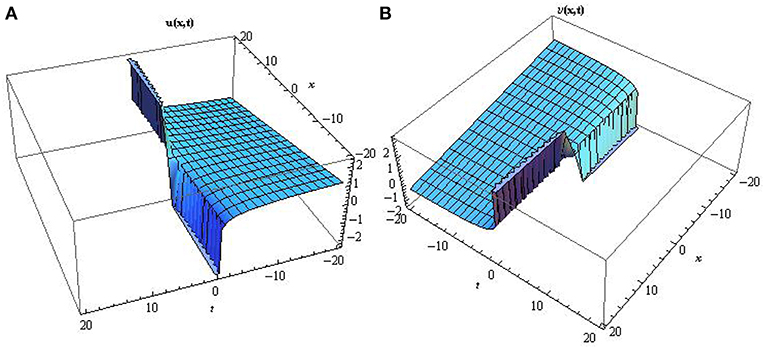
Figure 1. Surface profile of the algebraic functions solutions A and B mathematically represented by Equation (26) by setting c₁ = 0.5, c₂ = −0.2, c₃ = 0.2, d = 2.

FIGURE 2

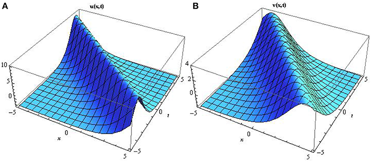
Figure 2. Surface profile of the non topological soliton solutions A and B mathematically represented by Equation (33) describing several terminologies in the field of mathematical physics by setting a₁ = 0.5, b₂ = −0.1, c₃ = 0.2, d = 2, e = 2, f = 0.4.

FIGURE 3

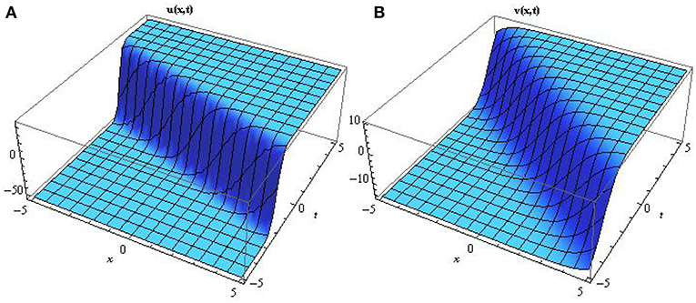
Figure 3. Surface profile of the topological soliton solutions A and B mathematically represented by Equation (40) describing several terminologies in the field of mathematical physics by setting a₁ = 0.4, b₂ = −0.2, c₃ = 0.1, d = 2, e = 2, f = 0.4.

FIGURE 4

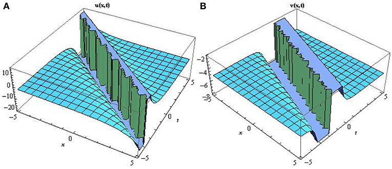
Figure 4. Surface profile of the singular soliton solutions type-I A and B mathematically represented by Equation (47) describing several terminologies in the field of mathematical physics by setting a₁ = 0.6, b₂ = −0.7, c₃ = 0.2, d = 1, e = 2, f = 0.4.

FIGURE 5

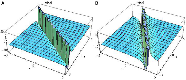
Figure 5. Surface profile of the singular soliton solutions type-I I A and B mathematically represented by Equation (54) describing several terminologies in the field of mathematical physics by setting a₁ = 0.2, b₂ = 0.8, c₃ = 0.2, d = 1, e = 2, f = 0.5.

Author Contributions

All authors listed have made a substantial, direct and intellectual contribution to the work, and approved it for publication.

Conflict of Interest Statement

The authors declare that the research was conducted in the absence of any commercial or financial relationships that could be construed as a potential conflict of interest.

References

1. Olver PJ. Application of Lie Groups to Differential Equations. Berlin: Springer (1986).

2. Galaktionov VA. Invariant subspaces and new explicit solutions to evolution equations with quadratic nonlinearities. Proc Roy Soc Endin Sect A. (1995) 125:225–46.

Google Scholar

3. Ma WX. A refined invariant subspace method and applications to evolution equations. Proc Roy Soc Endin ect A. (2012) 55:1769–78. doi: 10.1007/s11425-012-4408-9

CrossRef Full Text | Google Scholar

4. Shen SF, Qu CZ, Ji LN. Maximal dimension of invariant subspaces to system of nonlinear evolution equations. Chin Ann Math Ser B. (2012) 33:161–78. doi: 10.1007/s11401-012-0705-4

CrossRef Full Text | Google Scholar

5. Zhu CR, Qu CZ. Maximal dimension of invariant subspaces admitted by nonlinear vector differential operators. J Math Phys. (2011) 52:043507. doi: 10.1063/1.3574534

CrossRef Full Text | Google Scholar

6. Song J, Shen S, Jin Y, Zhang J. New maximal dimension of invariant subspaces to coupled systems with two-component equations. Commun Nonlinear Sci Numer Simulat. (2013) 18:2984–92. doi: 10.1016/j.cnsns.2013.03.019

CrossRef Full Text | Google Scholar

7. Biswas A, Green PD. Bright and dark optical solitons with time-dependent coefficients in a non-Kerr law media. Commun Nonlinear Sci Numer Simulat. (2012) 12:3865–73. doi: 10.1016/j.cnsns.2010.01.018

CrossRef Full Text | Google Scholar

8. Arshad M, Seadawy AR, Lu D. Bright-dark solitary wave solutions of generalized higher-order nonlinear Schrödinger equation and its applications in optics. J Electromagn Waves Appl. (2017) 31:1–11. doi: 10.1080/09205071.2017.1362361

CrossRef Full Text | Google Scholar

9. Zhou Q, Zhu Q, Yu H. Optical solitons in media with time-modulated nonlinearities and spatiotemporal dispersion. Nonlinear Dyn. (2015) 80:983–7. doi: 10.1007/s11071-015-1922-7

CrossRef Full Text | Google Scholar

10. Younis M, Younas U, Rehman SU. Optical bright-dark and Gaussian soliton with third order dispersion. Optik (2017) 134:233–8. doi: 10.1016/j.ijleo.2017.01.053

CrossRef Full Text | Google Scholar

11. Ma WX, Liu Y. Invariant subspaces and exact solutions of a class of dispersive evolution equations. Commun Nonlinear Sci Numer Simulat. (2012) 17:3795–801. doi: 10.1016/j.cnsns.2012.02.024

CrossRef Full Text | Google Scholar

12. Gurses M, Karasu A. Integrable coupled KdV systems. J Math Phys. (1998) 39:2103.

Google Scholar

13. Inc M, Hashemi MS, Aliyu AI. Exact solutions and conservation laws of the Bogoyavlenskii equation. Acta Physica Pol A. (2018) 133:1133–7. doi: 10.12693/APhysPolA.133.1133

CrossRef Full Text | Google Scholar

14. Aliyu AI, Inc M, Yusuf A, Baleanu D. Symmetry analysis, explicit solutions, and conservation laws of a sixth-order nonlinear ramani equation. Symmetry. (2018) 10:341. doi: 10.3390/sym10080341

CrossRef Full Text | Google Scholar

15. Baskonus HM, Koc DA, Bulut H. Dark and new travelling wave solutions to the nonlinear evolution equation. Optik (2016) 127:8043–55. doi: 10.1016/j.ijleo.2016.05.132

CrossRef Full Text | Google Scholar

16. Baskonus HM. New acoustic wave behaviors to the Davey-Stewartson equation with power-law nonlinearity arising in fluid dynamics. Nonlin Dyn. 86:177–83 (2016). doi: 10.1007/s11071-016-2880-4

CrossRef Full Text | Google Scholar

17. Bulut H, Sulaiman TA, Baskonus HM. Dark, bright and other soliton solutions to the Heisenberg ferromagnetic spin chain equation. Superlatt Microstruct. (2018) 123:12–9. doi: 10.1016/j.spmi.2017.12.009

CrossRef Full Text | Google Scholar

18. Baskonus HM, Bulut H, Sulaiman TA. Dark, bright and other optical solitons to the decoupled nonlinear Schrödinger equation arising in dual-core optical fibers. Opt Quantum Electron. (2018) 50:1–12. doi: 10.1007/s11082-018-1433-0

CrossRef Full Text | Google Scholar

19. Khalique CM, Mhlanga IE. Travelling waves and conservation laws of a (2+1)-dimensional coupling system with Korteweg-de Vries equation. Appl Math Nonlin Sci. (2018) 3:241–54. doi: 10.21042/AMNS.2018.1.00018

CrossRef Full Text | Google Scholar

20. Fokas AS, Liu QM. Asymptotic integrability of water waves. Phys Rev Lett. (1996) 77:2347–51.

PubMed Abstract | Google Scholar