Physics-Inspired Optimization for Quadratic Unconstrained Problems Using a Digital Annealer

1. Introduction

Discrete optimization problems have ubiquitous applications in various fields and, in particular, many NP-hard combinatorial optimization problems can be mapped to a quadratic Ising model [1] or, equivalently, to a quadratic unconstrained binary optimization (QUBO) problem. Such problems arise naturally in many fields of research, including finance [2], chemistry [3, 4], biology [5, 6], logistics and scheduling [7, 8], and machine learning [9–12]. For this reason, there is much interest in solving these problems efficiently, both in academia and in industry.

The impending end of Moore's law [13] signals that relying on traditional silicon-based computer devices is not expected to sustain the current computational performance growth rate. In light of this, interest in novel computational technologies has been steadily increasing. The introduction of a special-purpose quantum annealer by D-Wave Systems Inc. [14] was an effort in this direction, aimed at revolutionizing how computationally intensive discrete optimization problems are solved using quantum fluctuations.

Despite continued efforts to search for a scaling advantage of quantum annealers over algorithms on conventional off-the-shelf CMOS hardware, there is as yet no consensus. Efforts to benchmark quantum annealers against classical counterparts such as simulated annealing (SA) [15] have abounded [14, 16–30]. Although for some classes of synthetic problems a large speedup was initially found, those problems were subsequently shown to have a trivial logical structure, such that they can be solved more efficiently by more-powerful classical algorithms [31]. To the best of our knowledge, the only known case of speedup is a constant speedup for a class of synthetic problems [29] and, so far, there is no evidence of speedup for an industrial application. The hope is that future improvements to the quantum annealer and, in particular, to its currently sparse connectivity and low precision due to analog noise, will demonstrate the power of quantum effects in solving optimization problems [32, 33]. With the same goal in mind, researchers have been inspired to push the envelope for such problems on novel hardware, such as the coherent Ising machine [32], as well as on graphics processing units (GPU) [27, 28] and application-specific CMOS hardware [34, 35]. Similarly, efforts to emulate quantum effects in classical algorithms—often referred to as quantum- or physics-inspired methods—run on off-the-shelf CMOS hardware have resulted in sizable advances in the optimization domain (see, e.g., [30] for an overview of different algorithms).

Fujitsu Laboratories has recently developed application-specific CMOS hardware designed to solve fully connected QUBO problems (i.e., on complete graphs), known as the Digital Annealer (DA) [34, 35]. The DA hardware is currently able to treat Ising-type optimization problems of a size up to 1, 024 variables, with 26 and 16 bits of (fixed) precision for the biases and variable couplers, respectively. The DA's algorithm, which we refer to as “the DA”, is based on simulated annealing, but differs in several ways (see section 2), as well as in its ability to take advantage of the massive parallelization possible when using a custom, application-specific CMOS hardware. Previous efforts of running simulated annealing in parallel include executing different iterations in parallel on an AP1000 massively parallel distributed-memory multiprocessor [36, 37]. In addition to the DA, a version of the Digital Annealer, which we refer to as “the PTDA,” and which uses parallel tempering Monte Carlo [38–42] for the algorithmic engine is now available. In particular, it has been shown that physics-inspired optimization techniques such as simulated annealing and parallel tempering Monte Carlo typically outperform specialized quantum hardware [30] such as the D-Wave devices.

Much of the benchmarking effort has centered around spin glasses, a type of constraint satisfaction problem, in part due to their being the simplest of the hard Boolean optimization problems. Furthermore, application-based benchmarks from, for example, industry tend to be structured and, therefore, systematic benchmarking is difficult. As such, spin glasses have been used extensively to benchmark algorithms on off-the-shelf CPUs [43, 44], novel computing technologies such as quantum annealers [18, 20, 45, 46], and coherent Ising machines [32]. In this paper, we benchmark the DA and the PTDA on spin-glass problems, comparing them to simulated annealing [47] and parallel tempering Monte Carlo with isoenergetic cluster moves [48, 49] (a variant of Houdayer cluster updates [50] within the context of optimization and not the thermal simulation of spin-glass systems), both state-of-the-art, physics-inspired optimization algorithms. For other alternative classical optimization techniques used in the literature to solve QUBO problems, the interested reader is referred to Hen et al. [22], Mandrà et al. [30], and Rosenberg et al. [51].

The paper is organized as follows. Section 2 describes the algorithms we have benchmarked. In section 3 we probe the advantage of parallel-trial over single-trial Monte Carlo moves and in section 4 we discuss the methodology we have used for measuring time to solution. In section 5 we introduce the problems benchmarked. The experimental results are presented and discussed in section 6. Finally, our conclusions are presented in section 7. The parameters used for our benchmarking are given in Appendix.

2. Algorithms

In this paper, we compare several Monte Carlo (MC) algorithms and their use for solving optimization problems.

2.1. Simulated Annealing

Simulated annealing (SA) [15] is a generic algorithm with a wide application scope. The SA algorithm starts from a random initial state at a high temperature. Monte Carlo updates at decreasing temperatures are then performed. Note that the temperatures used follow a predefined schedule.

When the simulation stops, one expects to find a low-temperature state, ideally the global optimum (see Algorithm 1 for details). The high-temperature limit promotes diversification, whereas the low-temperature limit promotes intensification. To increase the probability of finding the optimum, this process is repeated multiple times (referred to as “runs”), returning the best state found. The computational complexity of each Monte Carlo sweep in SA is ${O}(N^2)$ for fully connected problems with N variables, because each sweep includes N update proposals, and each accepted move requires updating N effective fields, at a constant computational cost.

ALGORITHM 1

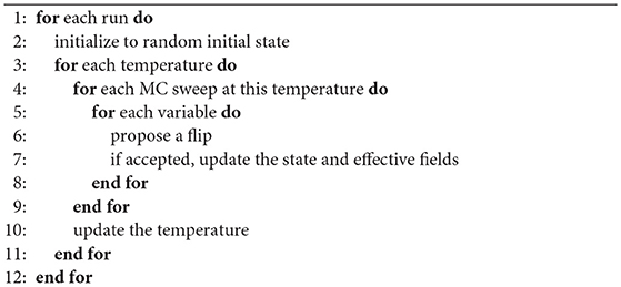
Algorithm 1. Simulated Annealing (SA)

2.2. The Digital Annealer's Algorithm

The DA's algorithmic engine [34, 35] is based on SA, but differs from it in three main ways (see Algorithm 2). First, it starts all runs from the same arbitrary state, instead of starting each run from a random state. This results in a small speedup due to its avoiding the calculation of the initial N effective fields and the initial energy for each run. Second, it uses a parallel-trial scheme in which each Monte Carlo step considers a flip of all variables (separately), in parallel. If at least one flip is accepted, one of the accepted flips is chosen uniformly at random and it is applied. Recall that in SA, each Monte Carlo step considers a flip of a single variable only (i.e., single trial). The advantage of the parallel-trial scheme is that it can boost the acceptance probability, because the likelihood of accepting a flip out of N flips is typically much higher than the likelihood of flipping a particular variable (see section 3). Parallel rejection algorithms on GPU [52, 53] are examples of similar efforts in the literature to address the low acceptance probability problem in Monte Carlo methods. Finally, the DA employs an escape mechanism called a dynamic offset, such that if no flip was accepted, the subsequent acceptance probabilities are artificially increased by subtracting a positive value from the difference in energy associated with a proposed move. This can help the algorithm to surmount short, narrow barriers.

ALGORITHM 2

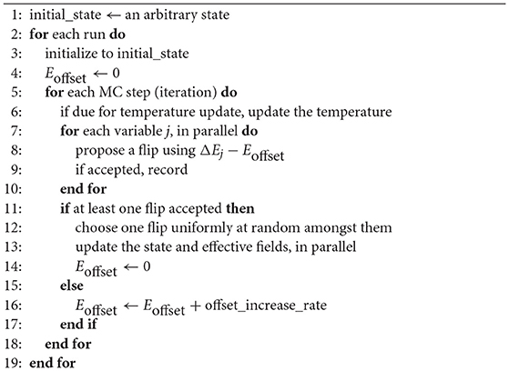
Algorithm 2. The Digital Annealer's Algorithm

Furthermore, the application-specific CMOS hardware allows for massive parallelization that can be exploited for solving optimization problems faster. For example, in the DA, evaluating a flip of all variables is performed in parallel, and when a flip is accepted and applied, the effective fields of all neighbors are updated in parallel. Note that this step requires a constant time, regardless of the number of neighbors, due to the parallelization on the hardware, whereas the computational time of the same step in SA increases linearly in the number of neighbors.

In order to understand the logic behind the DA, it is helpful to understand several architectural considerations that are specific to the DA hardware. In the DA, each Monte Carlo step takes the same amount of time, regardless of whether a flip was accepted (and therefore applied) or not. In contrast, in a CPU implementation of SA, accepted moves are typically much more computationally costly than rejected moves, that is, $[{O}(N)$ vs. ${O}(1)]$, due to the need to update N effective fields vs. none if the flip is rejected. As a result, in the DA, the potential boost in acceptance probabilities (from using the parallel-trial scheme) is highly desirable. In addition, in the DA, the computational complexity of updating the effective fields is constant regardless of the connectivity of the graph. Comparing this with SA, the computational complexity of updating the effective fields is ${O}(N)$ for fully connected graphs, but it is ${O}(d)$ for fixed-degree graphs (in which each node has d neighbors). Therefore, running SA on a sparse graph is typically faster than on a dense graph, but the time is the same for the DA. For this reason, it is expected that the speedup of the DA over SA be, in general, higher for dense graphs than for sparse ones.

2.3. Parallel Tempering With Isoenergetic Cluster Moves

In parallel tempering (PT) [38–42, 54] (also known as replica-exchange Monte Carlo), multiple replicas of the system are simulated at different temperatures, with periodic exchanges based on a Metropolis criterion between neighboring temperatures. Each replica, therefore, performs a random walk in temperature space, allowing it to overcome energy barriers by temporarily moving to a higher temperature. The higher-temperature replicas are typically at a high enough temperature that they inject new random states into the system, essentially re-seeding the algorithm continuously, obviating (at least partially) the need to perform multiple runs. PT has been used effectively in multiple research fields [41], and often performs better than SA, due to the increased mixing.

The addition of isoenergetic cluster moves (ICM) [48, 50] to PT, which flip multiple variables at a time, can allow for better exploration of the phase space, but only if the variable clusters do not span the whole system [48, 49]. ICM is a generalization of Houdayer's cluster algorithm, which was tailored for two-dimensional spin-glass problems [50]. To perform ICM, two copies (or more) of the system are simulated at the same temperature. The states of those two replicas are then compared, to find a cluster of variables (i.e., a connected component) that are opposite. In the case of QUBO problems, opposite variables are defined as having a product of zero. Finally, the move is applied by swapping the states of the opposite variables in the two replicas. The total energy of the two replicas is unchanged by this move, such that it is rejection free. The combination of PT and ICM, PT+ICM (also known as borealis; see Algorithm 3 [49]), has been shown to be highly effective for low-dimensionality spin-glass-like problems [20, 30, 55], but it does not provide a benefit for problems defined on fully connected graphs. This can be understood by noting that when the clusters span the system, ICM essentially results in swapping the states completely.

ALGORITHM 3

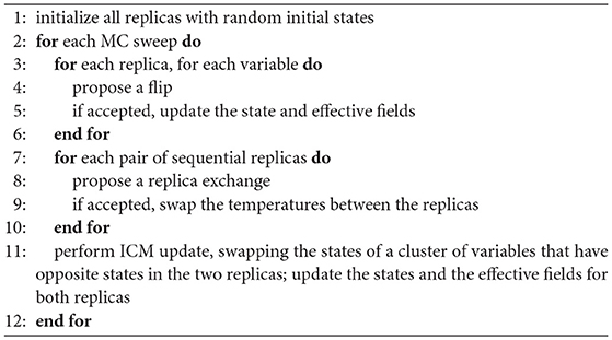
Algorithm 3. Parallel Tempering with Isoenergetic Cluster Moves (PT+ICM)

2.4. The Parallel Tempering Digital Annealer's Algorithm

Because the DA's algorithm is based on SA, and given the often superior results that PT gives over SA (see, e.g., [30]), Fujitsu Laboratories has also developed a Parallel Tempering Digital Annealer (PTDA). We had access to an early implementation of a PTDA. In the PTDA, the sweeps in each replica are performed as in the DA, including the parallel-trial scheme, parallel updates, and using the dynamic offset mechanism, but the PT moves are performed on a CPU. The temperatures are set automatically based on an adaptive scheme by Hukushima et al. [56]. In this scheme, the high and low temperatures are fixed, and intermediate temperatures are adjusted with the objective of achieving an equal replica-exchange probability for all adjacent temperatures. Having equal replica-exchange acceptance probabilities is a common target, although other schemes exist [42].

The next generation of the Digital Annealer is expected to be able to simulate problems on complete graphs up to 8, 192 variables in size, to have faster annealing times, and to perform the replica-exchange moves on the hardware, rather than on a CPU. This is significant, because when performing a computation in parallel, if a portion of the work is performed sequentially, it introduces a bottleneck that eventually dominates the overall run time (as the number of parallel threads is increased). Amdahl's Law [57] quantifies this by stating that if the sequential part is a fraction α of the total work, the speedup is limited to 1/α asymptotically.

3. Parallel-Trial vs. Single-Trial Monte Carlo

To illustrate the advantage of parallel-trial Monte Carlo updates as implemented in the DA over single-trial Monte Carlo updates, let us calculate their respective acceptance probabilities. The acceptance probability for a particular Monte Carlo move is given by the Metropolis criterion ${A}(\Delta E_i,T)\equiv e^{-\Delta E_i/T}$, where ΔE_i denotes the difference in energy associated with flipping variable i, and T is the temperature. The single-trial acceptance probability is then given by

$\begin{array}{rc}{{P}}_{\text{s}}(T)=\frac{1}{N}{\displaystyle \sum _i}{A}(\Delta E_i,T),& (1)\end{array}$

where N is the number of variables. In contrast, the parallel-trial acceptance probability is given by the complement probability of not accepting a move,

$\begin{array}{rc}{{P}}_{\text{p}}(T)=1-{\displaystyle \prod _i}\left[1-{A}(\Delta E_i,T)\right].& (2)\end{array}$

At low temperatures, we expect the acceptance probability to reach zero, in general. In the limit ${A}\to 0$, a first-order approximation of the parallel-trial acceptance probability gives

$\begin{array}{rc}{{P}}_{\text{p}}(T)\simeq {\displaystyle \sum _i}{A}(\Delta E_i,T).& (3)\end{array}$

This indicates that in the best case, there is a speedup by a factor of N at low temperatures. In contrast, at a high enough temperature, all moves are accepted, hence ${A}\to 1$. In this limit, it is clear that both the single-trial and parallel-trial acceptance probabilities reach 1, so parallel-trial Monte Carlo does not have an advantage over single-trial Monte Carlo.

To quantify the difference between parallel-trial and single-trial Monte Carlo, we perform a Monte Carlo simulation at constant temperature for a sufficiently large number of sweeps to reach thermalization. Once the system has thermalized, we measure the single-trial and parallel-trial acceptance probabilities at every move. This has been repeated for a number of sweeps, and for multiple temperatures and multiple problems.

The results of such an experiment are presented in Figure 1, for problems of size N = 64 of the four problem classes described in detail in section 5. The problem classes include two-dimensional (2D) and fully connected [Sherrington–Kirkpatrick (SK)] spin-glass problems with bimodal and Gaussian disorder. The results for all the problem classes except for the 2D-bimodal class follow the expected pattern of the acceptance probabilities reaching zero at low temperatures and one at high temperatures. In the 2D-bimodal case, there is a huge ground-state degeneracy, such that even at the ground state there are single variables for which a flip does not result in a change in energy. This results in a positive single-trial acceptance probability even at very low temperatures. For the same reason, the parallel-trial probability reaches one even for very low temperatures.

FIGURE 1

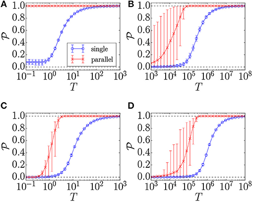
Figure 1. Mean single-trial and parallel-trial acceptance probabilities $({P})$ vs. the temperature (T), for four problem classes: (A) 2D-bimodal, (B) 2D-Gaussian, (C) SK-bimodal, and (D) SK-Gaussian. Error bars are given by the 5th and 95th percentiles of the acceptance probabilities in the configuration space. A constant-temperature Monte Carlo simulation has been run for 10⁵ sweeps to thermalize, after which the acceptance probabilities are measured for 5 · 10³ sweeps. For each problem class, the simulation has been performed on 100 problem instances of size N = 64 with 10 repeats per problem instance. The horizontal dashed lines show the minimum and maximum attainable probabilities, zero and one, respectively. Acceptance probabilities for the parallel-trial scheme approach unity as a function of simulation time considerably faster than in the single-trial scheme.

To quantify the acceptance probability advantage of parallel-trial over single-trial updates, it is instructive to study the parallel-trial acceptance probability divided by the single-trial acceptance probability, as presented in Figure 2. For all problem classes except 2D-bimodal, the advantage at low temperatures is indeed a factor of N, as suggested by dividing Equation 3 by Equation 1. As explained above, in the 2D-bimodal case the single-trial acceptance probability is non-negligible at low temperatures, leading to a reduced advantage. It is noteworthy that the advantage of the parallel-trial scheme is maximal at low temperatures, where the thermalization time is longer. As such, the parallel-trial scheme provides an acceptance probability boost where it is most needed.

FIGURE 2

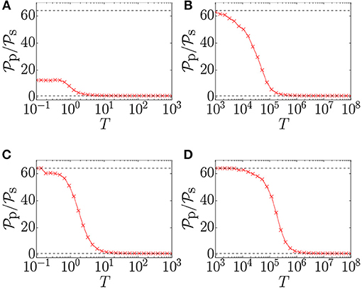
Figure 2. Ratio of the mean parallel-trial acceptance probability $({{P}}_{\mathrm{\text{p}}})$ to the mean single-trial acceptance probability $({{P}}_{\mathrm{\text{s}}})$ vs. the temperature (T), for four problem classes: (A) 2D-bimodal, (B) 2D-Gaussian, (C) SK-bimodal, and (D) SK-Gaussian. A constant-temperature Monte Carlo simulation has been run for 10⁵ sweeps to thermalize, after which the acceptance probabilities are measured for 5 · 10³ sweeps. For each problem class, the simulation has been performed on 100 problem instances of size N = 64 with 10 repeats per problem instance. The upper horizontal dashed line indicates N, the number of variables, which is the expected theoretical value of the ratio at low temperatures, as given by Equation 3 divided by Equation 1. The lower horizontal line indicates the minimum value of the ratio, which is one.

4. Scaling Analysis

The primary objective of benchmarking is to quantify how the computational effort in solving problems scales as the size of the problem (e.g., the number of variables) increases. The algorithms we consider here are all stochastic, and a common approach to measuring the scaling of a probabilistic algorithm is to measure the total time required for the algorithm to find a reference energy (cost) at least once with a probability of 0.99. The reference energy is represented by the optimal energy if available or, otherwise, by the best known energy. We denote this time to solution by “TTS,” and explain how it is calculated in the rest of this section.

We consider the successive runs of a probabilistic algorithm as being a sequence of binary experiments that might succeed in returning the reference energy with some probability. Let us formally define X₁, X₂, …, X_r as a sequence of random, independent outcomes of r runs (experiments), where ℙ(X_i = 1) = θ denotes the probability of success, that is, of observing the reference energy at the i-th run. Defining

$\begin{array}{rc}Y={\displaystyle \sum _{i=1}^r}{X}_i& (4)\end{array}$

as the number of successful observations in r runs, we have

$\begin{array}{ll}\mathbb{P}(Y=y|\theta ,r)=\left(\begin{array}{c}r\\ y\end{array}\right){(1-\theta )}^{r-y}{\theta }^y.& (5)\end{array}$

That is, Y has a binomial distribution with parameters r and θ. We denote the number of runs required to find the reference energy with a probability of 0.99 as R₉₉, which equals r such that ℙ(Y ≥ 1|θ, r) = 0.99. It can be verified that

$\begin{array}{rc}{\text{R}}_{99}=\frac{log(1-0.99)}{log(1-\theta )}& (6)\end{array}$

and, consequently, that

$\begin{array}{rc}\text{TTS}=\tau {\text{R}}_{99},& (7)\end{array}$

where τ is the time it takes to run the algorithm once. Because the probability of success θ is unknown, the challenge is in estimating θ.

Instead of using the sample success proportion as a point estimate for θ, we follow the Bayesian inference technique to estimate the distribution of the probability of success for each problem instance [22]. Having distributions of the success probabilities would be helpful in more accurately capturing the variance of different statistics of the TTS. In the Bayesian inference framework, we start with a guess on the distribution of θ, known as a prior, and update it based on the observations from consecutive runs of the algorithm in order to obtain the posterior distribution. Since the consecutive runs have a binomial distribution, the suitable choice of prior is a beta distribution [58] that is the conjugate prior of the binomial distribution. This choice guarantees that the posterior will also have a beta distribution. The beta distribution with parameters α = 0.5 and β = 0.5 (the Jeffreys prior) is chosen as a prior because it is invariant under reparameterization of the space and it learns the most from the data [59]. Updating the Jeffreys prior based on the observations from consecutive runs, the posterior distribution, denoted by π(θ), is π(θ) ~ Beta(α + y, β + r − y), where r is the total number of runs and y is the number of runs in which the reference energy is found.

To estimate the TTS for the entire population of instances with similar parameters, let us assume that there are I instances with the same number of variables. After finding the posterior distribution π_i(θ) for each instance i in set {1, 2, …, I}, we use bootstrapping to estimate the distribution of the q-th percentile of the TTS. This procedure is described in Algorithm 4.

ALGORITHM 4

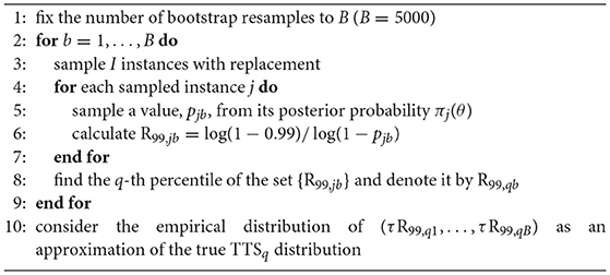
Algorithm 4. Estimating the Distribution of the q-th Percentile of the TTS

The procedure for deriving the TTS is slightly different for the DA and the PTDA. The anneal time of the algorithmic engine of the DA is not a linear function of the number of runs for a given number of sweeps. We therefore directly measure the anneal time for a given number of iterations and a given number of runs where the latter is equal to the R₉₉. Each iteration (Monte Carlo step) in the DA represents one potential update and each Monte Carlo sweep corresponds to N iterations.

It is important to note that the correct scaling is only observed if the parameters of the solver are tuned such that the TTS is minimized. Otherwise, a suboptimal scaling might be observed and incorrect conclusions could be made. Recall that the TTS is the product of the R₉₉ and the time taken per run τ. Let us consider a parameter that affects the computational effort taken, such as the number of sweeps. Increasing the number of sweeps results in the algorithm being more likely to find the reference solution, hence resulting in a lower R₉₉. On the other hand, increasing the number of sweeps also results in a longer runtime, increasing τ. For this reason, it is typical to find that the TTS reaches infinity for a very low or very high number of sweeps, and the goal is to experimentally find a number of sweeps at which the TTS is minimized.

5. Benchmarking Problems

A quadratic Ising model can be represented by a Hamiltonian (i.e., cost function) of the form

$\begin{array}{rc}{H}=-{\displaystyle \sum _{(i,j)\in E}}{J}_{ij}{s}_i{s}_j-{\displaystyle \sum _{i\in V}}{h}_i{s}_i.& (8)\end{array}$

Here, s_i ∈ {−1, 1} represent Boolean variables, and the problem is encoded in the biases h_i and couplers J_ij. The sums are over the vertices V and weighted edges E of a graph G = (V, E). It can be shown that the problem of finding a spin configuration {s_i} that minimizes ${H}$, in general, is equivalent to the NP-hard weighted max-cut problem [60–63]. Spin glasses defined on nonplanar graphs fall into the NP-hard complexity class. However, for the special case of planar graphs, exact, polynomial-time methods exist [64].

The algorithmic engine of the Digital Annealer can optimize instances of QUBO problems in which the variables x_i take values from {0, 1} instead of {−1, 1}. To solve a quadratic Ising problem described by the Hamiltonian represented in Equation 8, we can transform it into a QUBO problem by taking s_i = 2x_i − 1.

In the following, we explain the spin-glass problems used for benchmarking.

2D-bimodal—Two-dimensional spin-glass problems on a torus (periodic boundaries), where couplings are chosen according to a bimodal distribution, that is, they take values from {−1, 1} with equal probability.

2D-Gaussian—Two-dimensional spin-glass problems where couplings are chosen from a Gaussian distribution with a mean of zero and a standard deviation of one, scaled by 10⁵.

SK-bimodal—Spin-glass problems on a complete graph—also known as Sherrington–Kirkpatrick (SK) spin-glass problems [65]—where couplings are chosen according to a bimodal distribution, that is, they take values from {−1, 1} with equal probability.

SK-Gaussian—SK spin-glass problems where couplings are chosen from a Gaussian distribution with a mean of zero and a standard deviation of one, scaled by 10⁵.

In all the problems, the biases are zero. The coefficients of the 2D-Gaussian and SK-Gaussian problems are beyond the precision limit of the current DA. In order to solve these problems using the DA, we have used a simple scheme to first scale the coefficients up to their maximum limit and then round to the nearest integer values. The maximum values for the linear and quadratic coefficients are given by the precision limits of the current DA hardware, that is, 2²⁵ − 1 and 2¹⁵ − 1, respectively. The problem instances are not scaled when solving them using SA or PT (PT+ICM).

Our benchmarking experiment has been parameterized by the number of variables. Specifically, we have considered nine different problem sizes in each problem category and generated 100 random instances for each problem size. We have used the instance generator provided by the University of Cologne Spin Glass Server¹ to procure the 2D-bimodal and 2D-Gaussian instances. SK instances with bimodal and Gaussian disorder have been generated as described above. Each problem instance has then been solved by different Monte Carlo algorithms. Optimal solutions to the 2D-bimodal and 2D-Gaussian problems have been obtained by a branch-and-cut [66] technique available via the Spin Glass Server ¹. The SK problems are harder than the two-dimensional problems and the server does not find the optimal solution within the 15-min time limit. For the SK-bimodal and the SK-Gaussian problems with 64 variables, we have used a semidefinite branch-and-bound technique through the Biq Mac Solver [67] and BiqCrunch [68] to find the optimal solutions, respectively. For problems of a size greater than 64, the solution obtained by PT with a large number of sweeps (5 · 10⁵ sweeps) is considered a good upper bound for the optimal solution. We refer to the optimal solution (or its upper bound) as the reference energy.

6. Results and Discussion

In this paper, we have used an implementation of the PT (and PT+ICM) algorithm based on the work of Zhu et al. [48, 49]. The DA and PTDA algorithms are run on Fujitsu's Digital Annealer hardware. For the SA simulations we have used the highly optimized, open source code by Isakov et al. [47].

The DA solves only a fully connected problem where the coefficients of the absent vertices and edges in the original problem graph are set to zero. In our benchmarking study, we have included both two-dimensional and SK problems to represent the two cases of sparsity and full connectivity, respectively. Furthermore, we have considered both bimodal and Gaussian disorder in order to account for problems with high or low ground-state degeneracy. The bimodal disorder results in an energy landscape that has a large number of free variables with zero effective local fields. As a result, the degeneracy of the ground state increases exponentially in the number of free variables, making it easier for any classical optimization algorithm to reach a ground state. Problem instances that have Gaussian coefficients further challenge the DA, due to its current limitations in terms of precision.

In what follows, we discuss our benchmarking results, comparing the performance of different algorithms using two-dimensional and SK spin-glass problems, with bimodal and Gaussian disorder. We further investigate how problem density affects the DA's performance. The parameters of the algorithms used in this benchmarking study are presented in Appendix.

6.1. 2D Spin-Glass Problems

Figure 3 illustrates the TTS results of the DA, SA, PT+ICM, and PTDA for 2D spin-glass problems with bimodal and Gaussian disorder. In all TTS plots in this paper, points and error bars represent the mean and the 5th and 95th percentiles of the TTS distribution, respectively. PT+ICM has the lowest TTS for problems with bimodal and Gaussian disorder and has a clear scaling advantage. In problems with bimodally distributed couplings, although SA results in a lower TTS for small-sized problems, the DA and SA demonstrate similar TTSs as the problem size increases. The performance of both SA and the DA decreases when solving harder problem instances with Gaussian disorder, with significantly reduced degeneracy of the ground states. However, in this case, the DA outperforms SA even with its current precision limit.

FIGURE 3

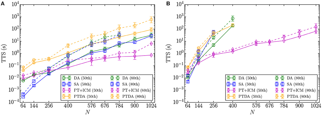
Figure 3. Mean, 5th, and 95th percentiles of the TTS distributions (TTS₅₀ and TTS₈₀) for (A) 2D-bimodal and (B) 2D-Gaussian spin-glass problems. For some problem sizes N, the percentiles are smaller than the symbols.

The PTDA yields higher TTSs than the DA in both cases of bimodal and Gaussian disorder, likely due to the CPU overhead of performing parallel tempering moves. Considering the number of problems solved to optimality, the PTDA outperforms the DA when solving 2D spin-glass problems with bimodal couplings; however, as shown in Figure 3, the PTDA solves fewer problems with Gaussian disorder.

In order to estimate the q-th percentile of the TTS distribution, at least q% of problems should be solved to their corresponding reference energies. If there is no point for a given problem size and an algorithm in Figure 3, it means that enough instances have not been solved to their reference energies and we therefore could not estimate the TTS percentiles. Increasing the number of iterations to 10⁷ in the DA and the PTDA, we could not solve more than 80% of the 2D-Gaussian problem instances with a size greater than or equal to 400. Therefore, to gather enough statistics to estimate the 80th percentile of the TTS, we have increased the number of iterations to 10⁸ in the DA. However, because of the excessive resources needed, we have not run the PTDA with such a large number of iterations.

2D-Bimodal

In Figure 4A, we observe that for a given problem size and number of sweeps, the DA reaches higher success probabilities than SA. As the problem size increases, the difference between the mean success probability curves of the DA and SA becomes less pronounced. Figure 4B illustrates the success probability correlation of 100 problem instances of size 1, 024. The DA yields higher success probabilities for 52 problem instances out of 100 instances solved.

FIGURE 4

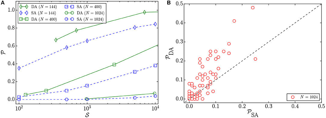
Figure 4. (A) Mean success probabilities (${P}$) of 2D-bimodal instances vs. the number of Monte Carlo sweeps (${S}$) for different problem sizes N solved by the DA and SA. The error bars are not included, for better visibility. (B) Success probability correlation plot of 100 2D-bimodal instances with N = 1, 024 variables, where the number of sweeps is 10⁴ for SA and the number of iterations is 10⁷ for the DA. Because each sweep corresponds to N = 1, 024 iterations, the number of sweeps is ≃10⁴ for the DA, as well.

For 2D-bimodal problems, the boost in the probability of updating a single variable due to the parallel-trial scheme is not effective enough to decrease the TTS or to result in better scaling (Figure 3A). Since both the DA and SA update at most one variable at a time, increasing the probability of updating a variable in a problem with bimodal disorder, where there are a large number of free variables, likely results in a new configuration without lowering the energy value (see section 3 for details).

2D-Gaussian

The performance of the DA and SA significantly degrades when solving the problems with Gaussian disorder, which are harder; however, the DA demonstrates clear superiority over SA. Figure 5 shows the residual energy (${E}$), which is the relative energy difference (in percent) between the lowest-energy solution found and the reference-energy solution, for the largest problem size, which has 1, 024 variables. We observe that the DA outperforms SA, as it results in a lower residual energy for a given number of Monte Carlo sweeps (${S}\le 10^5$). Furthermore, Figure 6 illustrates that the parallel-trial scheme is more effective for this class of problems, which could be due to the decrease in the degeneracy of the ground states. In Figure 6A, we observe that the difference between mean success probabilities, for a problem of size 144 with 10⁴ Monte Carlo sweeps, is larger compared to the bimodal disorder (Figure 4A). The success probability correlation of 100 2D-Gaussian problem instances with 400 variables in Figure 6B further demonstrates that the DA reaches higher success probabilities, which results in a lower TTS (Figure 3B).

FIGURE 5

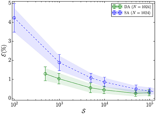
Figure 5. Mean, 5th, and 95th percentiles of the residual energy (${E}$) vs. number of Monte Carlo sweeps (${S}$) for 2D-Gaussian problem instances with N = 1, 024 variables solved by the DA and SA. As the number of Monte Carlo sweeps approaches infinity, the residual energy of both algorithms will eventually reach zero. We have run SA for up to 10⁶ sweeps and the DA for up to 10⁸ iterations (10⁸/1024 ~ 10⁵ sweeps). Therefore, the data up to 10⁵ sweeps is presented for both algorithms. We expect that by increasing the number of iterations to 10⁹ (10⁶ sweeps) in the DA, the residual energy would further decrease.

FIGURE 6

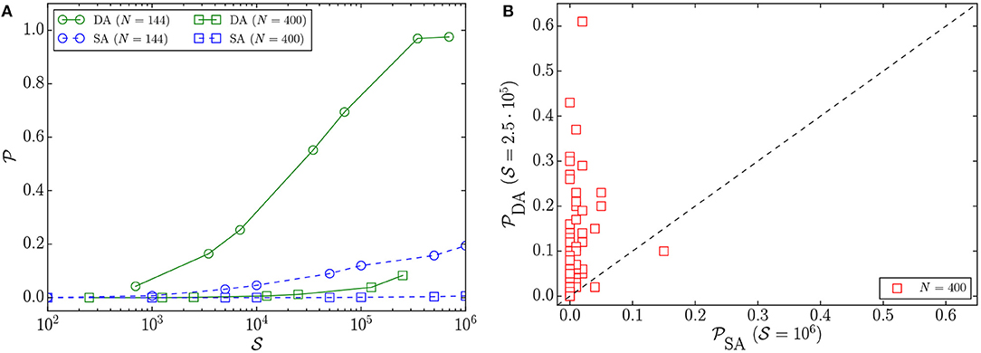
Figure 6. (A) Mean success probabilities (${P}$) vs. the number of Monte Carlo sweeps (${S}$) for 2D-Gaussian problem instances with N = 144 and N = 400 variables solved by the DA and SA. The error bars are not included, for better visibility. (B) The success probability correlation of 100 2D-Gaussian instances with N = 400 variables. The data points are obtained considering 10⁶ and 2.5 · 10⁵ Monte Carlo sweeps for SA and the DA, respectively.

6.2. SK Spin-Glass Problems

We have solved the SK problem instances with the DA, SA, PT, and the PTDA. As explained in section 2, for the fully connected problems, the cluster moves have not been included in PT because the clusters of variables span the entire system. Our initial experiments verified that adding ICM to PT increases the computational cost without demonstrating any scaling benefit for this problem class.

The statistics of the TTS distribution of the DA, the PTDA, and the SA and PT algorithms are shown in Figure 7A for SK-bimodal problem instances. Comparing the DA to SA and PT, we observe that the DA yields a noticeable, consistent speedup of at least two orders of magnitude as we approach the largest problem size. In the fully connected problems, accepting a move and updating the effective local fields in a CPU implementation of a Monte Carlo algorithm is computationally more expensive than for sparse problems.

FIGURE 7

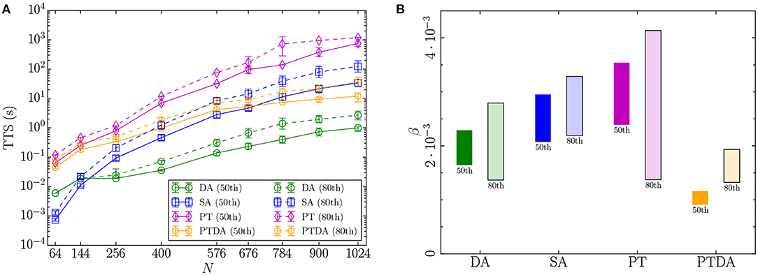
Figure 7. (A) Mean, 5th, and 95th percentiles of the TTS distributions (TTS₅₀ and TTS₈₀) for fully connected spin-glass problems with bimodal disorder. For some problem sizes, the percentiles are smaller than the symbols. (B) The 90% confidence interval of the estimated scaling exponent β based on the mean of the TTS₅₀ and TTS₈₀ for the SK-bimodal problem class. The label below each rectangle represents the TTS percentile on which the confidence interval is based. For each algorithm, the five largest problem sizes have been used to estimate the scaling exponent by fitting a linear model to log₁₀ TTS. The R² of the fitted model is greater than or slightly lower than 90% for each algorithm.

Figure 7A shows that each algorithm has solved at least 80% of the SK instances for all problem sizes. We attribute this to the fact that the reference energy for the complete graph problems is an upper bound on the exact optimal solution. We do not know how tight the upper bound is, but it represents, to the best of our knowledge, the best known solution.

To obtain insights on scaling, for each algorithm, we have fit an exponential function of the form y = 10^α+βN, where y and N are the means of the TTS distribution and the number of variables, respectively. Figure 7B shows the 90% confidence interval of the estimated scaling exponent β for the algorithms based on the statistics of the 50th and the 80th percentiles of the TTS distribution. For the 50th percentile, we observe that the PTDA yields superior scaling over the other three algorithms for the problem class with bimodal disorder. For the 80th percentile, there is not enough evidence to draw a strong conclusion on which algorithm scales better because the 90% confidence intervals of the estimated scaling exponents overlap. However, the PTDA has the lowest point estimate.

For the DA, SA, and PT algorithms, we have searched over a large number of parameter combinations to experimentally determine a good set of parameters (see Appendix) while the parameters of the PTDA have been determined automatically by the hardware. We have further experimentally determined the optimal number of sweeps for all four algorithms. However, we do not rule out the possibility that the scaling of the algorithms might be suboptimal due to a non-optimal tuning of parameters. For example, the scaling of the PTDA might improve after tuning its parameters and PT might exhibit better scaling using a more optimized temperature schedule.

Figure 8 illustrates the TTS statistics and the confidence interval of the scaling exponent for SK-Gaussian problem instances solved by the DA, SA, PT, and the PTDA. We observe that the DA continues to exhibit a constant speedup of at least two orders of magnitude over the other algorithms, with no strong scaling advantage, in solving spin-glass problems with Gaussian disorder.

FIGURE 8

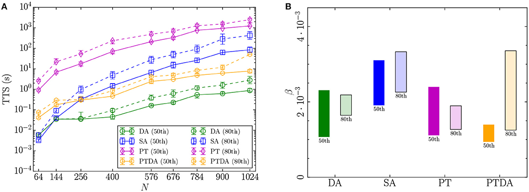
Figure 8. (A) Mean, 5th, and 95th percentiles of the TTS distributions (TTS₅₀ and TTS₈₀) for fully connected spin-glass problems with Gaussian disorder. For some problem sizes, the percentiles are smaller than the symbols. (B) The 90% confidence interval of the estimated scaling exponent β based on the mean of the TTS₅₀ and TTS₈₀ for the SK-Gaussian problem class. The label below each rectangle represents the TTS percentile on which the confidence interval is based. For each algorithm, the five largest problem sizes have been used to estimate the scaling exponent by fitting a linear model to log₁₀ TTS. The R² of the fitted model is greater than or slightly lower than 90% for each algorithm.

The DA vs. SA

The DA results in lower TTSs than SA for both SK-bimodal and SK-Gaussian problem instances. The reasons for this behavior are two-fold. First, the anneal time for the DA is independent of the number of variables and the density of the problem, whereas the computation time of a sweep in SA increases with the problem size and the problem density. Second, as shown in Figure 9, the parallel-trial scheme significantly improves the success probability in fully connected spin-glass problems of size 1, 024 with both bimodal and Gaussian disorder. As expected, the boost in the low-degeneracy problem instances (with Gaussian coefficients) is higher.

FIGURE 9

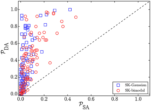
Figure 9. Success probability correlation (${P}$) of 100 SK instances of size 1, 024 with bimodal and Gaussian disorder. The number of Monte Carlo sweeps in SA is 10⁴ and the number of iterations in the DA is 10⁷, corresponding to ≃10⁴ Monte Carlo sweeps.

Although the confidence intervals of the scaling exponents overlap, considering the statistics of the TTS₈₀, the DA yields lower point estimates than SA for SK-bimodal and SK-Gaussian problems. In particular, β = 0.0021(7) [0.0019(3)] for the DA with bimodal [Gaussian] disorder, whereas β = 0.0027(6) [0.0028(5)] for SA with bimodal [Gaussian] disorder, thus providing a weak scaling advantage.

Our results on spin-glass problems with Gaussian disorder further indicate that the 16-bit precision of the hardware used in this study is not a limiting factor because the DA outperforms SA on instances of these problems. Since there is a high variance in the couplers of spin-glass instances with Gaussian disorder, we expect that the energy gap between the ground state and the first-excited state is likely greater than 10⁻⁵ and, as a result, the scaling/rounding effect is not significant [69]. Our experimentation data on the prototype of the second-generation Digital Annealer, which has 64 bits of precision on both biases and couplers, also confirms that the higher precision by itself does not have a significant impact on the results presented in this paper. We leave a presentation of our experimental results using the second-generation hardware for future work.

6.3. Spin-Glass Problems With Different Densities

Our results for the two limits of the problem-density spectrum suggest that the DA exhibits similar TTSs to SA on sparse problems, and outperforms SA on fully connected problems by a TTS speedup of approximately two orders of magnitude. To obtain a deeper understanding of the relation between the performance and the density, we have performed an experiment using random problem graphs with nine different densities. For each problem density, 100 problem instances with 1, 024 variables have been generated based on the Erdős–Rényi model [70], with bimodally distributed coupling coefficients, and zero biases. The parameters of the DA and SA have been experimentally tuned for each of the nine problem densities (see Appendix).

Figure 10 shows the statistics of the TTS of the DA and SA for different problem densities. The TTS results for 2D-bimodal (d = 0.4%) and SK-bimodal (d = 100%) for a problem size of 1, 024, representing the limits of the density spectrum, are also included. The DA has lower TTSs than SA for all problem densities except for the sparsest problem set—2D-bimodal. Not enough 2D-bimodal instances were solved to optimality using the DA and SA in order to estimate the statistics of the TTS₈₀ distributions.

FIGURE 10

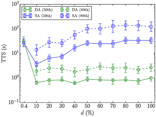
Figure 10. Mean, 5th, and 95th percentiles of the TTS distributions (TTS₅₀ and TTS₈₀) for spin-glass problems with different densities (d).

Figure 11 shows the success probabilities of 100 spin-glass problem instances of size 1, 024 with different densities solved by the DA and SA. The DA has higher success probabilities than SA by a statistically significant margin for all of the densities except for the sparsest problem set—2D-bimodal. We interpret these results as being due to both the increase in the success probabilities from using a parallel-trial scheme and the constant time required to perform each Monte Carlo step on the DA hardware architecture.

FIGURE 11

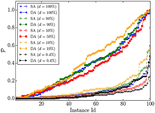
Figure 11. Success probabilities (${P}$) of 100 spin-glass problem instances with different densities solved by the SA and the DA algorithms. The number of Monte Carlo sweeps in SA is 10⁴ and the number of iterations in the DA is 10⁷, corresponding to ≃10⁴ Monte Carlo sweeps.

7. Conclusions and Outlook

In this work we have compared the performance of the Digital Annealer (DA) and the Parallel Tempering Digital Annealer (PTDA) to parallel tempering Monte Carlo with and without isoenergetic cluster moves (PT+ICM and PT, respectively) and simulated annealing (SA) using random instances of sparse and fully connected spin-glass problems, with bimodal and Gaussian disorder.

Our results demonstrate that the DA is approximately two orders of magnitude faster than SA and PT in solving dense problems, while it does not exhibit a speedup for sparse problems. In the latter problem class, the addition of cluster updates to the PT algorithm is very effective in traversing the energy barriers, outperforming algorithms that act on a single flip neighborhood, such as the DA and SA. For dense problems, the efficiency of the cluster moves diminishes such that the DA is faster, due to the parallel-trial scheme combined with the massive parallelization that is possible on application-specific CMOS hardware. Our results further support the position that the DA has an advantage over SA on random spin-glass problems with densities of 10% or higher.

In section 3 we demonstrate that parallel-trial Monte Carlo can offer a significant boost to the acceptance probabilities over standard updating schemes. Furthermore, we show that this boost vanishes at high temperatures and is diminished for problems with high ground-state degeneracy. Our benchmarking results further support the view that the parallel-trial scheme is more effective in solving problems with low ground-state degeneracy because an accepted move is more likely not only to change the state configuration, but also to lower the energy value.

In the current early implementation of the PTDA, the TTS is higher than it is likely to be in the future, due to the CPU overhead in performing PT moves. However, the PTDA algorithm demonstrates better scaling than the other three algorithms for a fully connected spin-glass problem of average computational difficulty, with bimodal couplings.

In the next generation of the Digital Annealer, the hardware architecture is expected to allow the optimization of problems using up to 8192 fully connected variables. In addition, the annealing time is expected to decrease, and we conjecture that the TTS might decrease accordingly. Finally, we expect the replica-exchange moves in the PTDA to be performed on the hardware, which could improve the performance of the PTDA.

Our results demonstrate that pairing application-specific CMOS hardware with physics-inspired optimization methods results in extremely efficient, special-purpose optimization machines. Because of their fully connected topology and high digital precision, these machines have the potential to outperform current analog quantum optimization machines. Pairing such application-specific CMOS hardware with a fast interconnect could result in large-scale transformative optimization devices. We thus expect future generations of the Digital Annealer to open avenues for the study of fundamental physics problems and industrial applications that were previously inaccessible with conventional CPU hardware.

Author Contributions

MA, GR, and HK developed the methodology, implemented the code, performed the experiments, analyzed the results, and wrote the manuscript. EV partially contributed to implementing the code and conducting the experiments. TM and HT carried out the experiments related to the PTDA algorithm.

Funding

This research was supported by 1QBit, Fujitsu Laboratories Ltd., and Fujitsu Ltd. The research of HK was supported by the National Science Foundation (Grant No. DMR-1151387). HK's research is based upon work supported by the Office of the Director of National Intelligence (ODNI), Intelligence Advanced Research Projects Activity (IARPA), via Interagency Umbrella Agreement No. IA1-1198. The views and conclusions contained herein are those of the authors and should not be interpreted as necessarily representing the official policies or endorsements, either expressed or implied, of the ODNI, IARPA, or the U.S. Government. The U.S. Government is authorized to reproduce and distribute reprints for Governmental purposes notwithstanding any copyright annotation thereon.

Conflict of Interest Statement

The authors declare that the research was conducted in the absence of any commercial or financial relationships that could be construed as a potential conflict of interest.

Acknowledgments

The authors would like to thank Salvatore Mandrà for helpful discussions, Lester Szeto, Brad Woods, Rudi Plesch, Shawn Wowk, and Ian Seale for software development and technical support, Marko Bucyk for editorial help, and Clemens Adolphs for reviewing the manuscript. We thank Zheng Zhu for providing us with his implementation of the PT+ICM algorithm [48, 49], and Sergei Isakov for the use of his implementation of the SA algorithm [47]. HK would like to thank Bastani Sonnati for inspiration.

Supplementary Material

The Supplementary Material for this article can be found online at: https://www.frontiersin.org/articles/10.3389/fphy.2019.00048/full#supplementary-material

Footnotes

1. ^http://informatik.uni-koeln.de/spinglass

References

1. Lucas A. Ising formulations of many NP problems. Front Phys. (2014) 12:5. doi: 10.3389/fphy.2014.00005

CrossRef Full Text | Google Scholar

2. Rosenberg G, Haghnegahdar P, Goddard P, Carr P, Wu K, de Prado ML. Solving the optimal trading trajectory problem using a quantum annealer. IEEE J Select Top Signal Process. (2016) 10:1053. doi: 10.1109/JSTSP.2016.2574703

CrossRef Full Text | Google Scholar

3. Hernandez M, Zaribafiyan A, Aramon M, Naghibi M. A novel graph-based approach for determining molecular similarity. arXiv:1601.06693. (2016).

Google Scholar

4. Hernandez M, Aramon M. Enhancing quantum annealing performance for the molecular similarity problem. Quantum Inform Process. (2017) 16:133. doi: 10.1007/s11128-017-1586-y

CrossRef Full Text | Google Scholar

5. Perdomo-Ortiz A, Dickson N, Drew-Brook M, Rose G, Aspuru-Guzik A. Finding low-energy conformations of lattice protein models by quantum annealing. Sci Rep. (2012) 2:571. doi: 10.1038/srep00571

PubMed Abstract | CrossRef Full Text | Google Scholar

6. Li RY, Di Felice R, Rohs R, Lidar DA. Quantum annealing versus classical machine learning applied to a simplified computational biology problem. NPJ Quantum Inf. (2018) 4:14. doi: 10.1038/s41534-018-0060-8

PubMed Abstract | CrossRef Full Text | Google Scholar

7. Venturelli D, Marchand DJJ, Rojo G. Quantum annealing implementation of job-shop scheduling. arXiv:1506.08479v2. (2015).

Google Scholar

8. Neukart F, Von Dollen D, Compostella G, Seidel C, Yarkoni S, Parney B. Traffic flow optimization using a quantum annealer. Front ICT. (2017) 4:29. doi: 10.3389/fict.2017.00029

CrossRef Full Text | Google Scholar

9. Crawford D, Levit A, Ghadermarzy N, Oberoi JS, Ronagh P. Reinforcement learning using quantum Boltzmann machines. arXiv:1612.05695v2. (2016).

Google Scholar

10. Khoshaman A, Vinci W, Denis B, Andriyash E, Amin MH. Quantum variational autoencoder. Quantum Sci Technol. (2019) 4:014001. doi: 10.1088/2058-9565/aada1f

CrossRef Full Text | Google Scholar

11. Henderson M, Novak J, Cook T. Leveraging adiabatic quantum computation for election forecasting. arXiv:1802.00069. (2018).

Google Scholar

12. Levit A, Crawford D, Ghadermarzy N, Oberoi JS, Zahedinejad E, Ronagh P. Free energy-based reinforcement learning using a quantum processor. arXiv:1706.00074. (2017).

Google Scholar

13. Moore G. Cramming more components onto integrated circuits. Electron Mag. (1965) 38:114.

Google Scholar

14. Johnson MW, Amin MHS, Gildert S, Lanting T, Hamze F, Dickson N, et al. Quantum annealing with manufactured spins. Nature. (2011) 473:194–8. doi: 10.1038/nature10012

PubMed Abstract | CrossRef Full Text | Google Scholar

15. Kirkpatrick S, Gelatt CD Jr, Vecchi MP. Optimization by simulated annealing. Science. (1983) 220:671–80. doi: 10.1126/science.220.4598.671

PubMed Abstract | CrossRef Full Text | Google Scholar

16. Dickson NG, Johnson MW, Amin MH, Harris R, Altomare F, Berkley AJ, et al. Thermally assisted quantum annealing of a 16-qubit problem. Nat Commun. (2013) 4:1903. doi: 10.1038/ncomms2920

PubMed Abstract | CrossRef Full Text | Google Scholar

17. Boixo S, Rønnow TF, Isakov SV, Wang Z, Wecker D, Lidar DA, et al. Evidence for quantum annealing with more than one hundred qubits. Nat Phys. (2014) 10:218–24. doi: 10.1038/nphys2900

CrossRef Full Text | Google Scholar

18. Katzgraber HG, Hamze F, Andrist RS. Glassy chimeras could be blind to quantum speedup: designing better benchmarks for quantum annealing machines. Phys Rev X. (2014) 4:021008. doi: 10.1103/PhysRevX.4.021008

CrossRef Full Text | Google Scholar

19. Rønnow TF, Wang Z, Job J, Boixo S, Isakov SV, Wecker D, et al. Defining and detecting quantum speedup. Science (2014) 345:420. doi: 10.1126/science.1252319

PubMed Abstract | CrossRef Full Text | Google Scholar

20. Katzgraber HG, Hamze F, Zhu Z, Ochoa AJ, Munoz-Bauza H. Seeking quantum speedup through spin glasses: the good, the bad, and the ugly. Phys Rev X. (2015) 5:031026. doi: 10.1103/PhysRevX.5.031026

CrossRef Full Text | Google Scholar

21. Heim B, Rønnow TF, Isakov SV, Troyer M. Quantum versus classical annealing of Ising spin glasses. Science. (2015) 348:215. doi: 10.1126/science.1252319

PubMed Abstract | CrossRef Full Text | Google Scholar

22. Hen I, Job J, Albash T, Rønnow TF, Troyer M, Lidar DA. Probing for quantum speedup in spin-glass problems with planted solutions. Phys Rev A. (2015) 92:042325. doi: 10.1103/PhysRevA.92.042325

CrossRef Full Text | Google Scholar

23. Albash T, Rønnow TF, Troyer M, Lidar DA. Reexamining classical and quantum models for the D-Wave One processor. Eur Phys J Spec Top. (2015) 224:111. doi: 10.1140/epjst/e2015-02346-0

CrossRef Full Text | Google Scholar

24. Martin-Mayor V, Hen I. Unraveling quantum annealers using classical hardness. Nat Sci Rep. (2015) 5:15324. doi: 10.1038/srep15324

PubMed Abstract | CrossRef Full Text | Google Scholar

25. Marshall J, Martin-Mayor V, Hen I. Practical engineering of hard spin-glass instances. Phys Rev A. (2016) 94:012320. doi: 10.1103/PhysRevA.94.012320

CrossRef Full Text | Google Scholar

26. Denchev VS, Boixo S, Isakov SV, Ding N, Babbush R, Smelyanskiy V, et al. What is the computational value of finite range tunneling? Phys Rev X. (2016) 6:031015. doi: 10.1103/PhysRevX.6.031015

CrossRef Full Text | Google Scholar

27. King J, Yarkoni S, Raymond J, Ozfidan I, King AD, Nevisi MM, et al. Quantum annealing amid local ruggedness and global frustration. arXiv:quant-phys/1701.04579v2. (2017).

Google Scholar

28. Albash T, Lidar DA. Demonstration of a scaling advantage for a quantum annealer over simulated annealing. Phys Rev X. (2018) 8:031016. doi: 10.1103/PhysRevX.8.031016

CrossRef Full Text | Google Scholar

29. Mandrà S, Katzgraber HG. A deceptive step towards quantum speedup detection. QST. (2018) 3:04LT01. doi: 10.1088/2058-9565/aac8b2

CrossRef Full Text | Google Scholar

30. Mandrà S, Zhu Z, Wang W, Perdomo-Ortiz A, Katzgraber HG. Strengths and weaknesses of weak-strong cluster problems: a detailed overview of state-of-the-art classical heuristics versus quantum approaches. Phys Rev A. (2016) 94:022337. doi: 10.1103/PhysRevA.94.022337

CrossRef Full Text | Google Scholar

31. Mandrà S, Katzgraber HG. The pitfalls of planar spin-glass benchmarks: raising the bar for quantum annealers (again). Quantum Sci Technol. (2017) 2:038501. doi: 10.1088/2058-9565/aa7877

CrossRef Full Text | Google Scholar

32. Hamerly R, Inagaki T, McMahon PL, Venturelli D, Marandi A, Onodera T, et al. Scaling advantages of all-to-all connectivity in physical annealers: the coherent Ising machine vs. D-Wave 2000Q. arXiv:quant-phys/1805.05217. (2018).

Google Scholar

33. Katzgraber HG, Novotny MA. How small-world interactions can lead to improved quantum annealer designs. Phys Rev Appl. (2018) 10:054004. doi: 10.1103/PhysRevApplied.10.054004

CrossRef Full Text | Google Scholar

34. Matsubara S, Tamura H, Takatsu M, Yoo D, Vatankhahghadim B, Yamasaki H, et al. Ising-model optimizer with parallel-trial bit-sieve engine. In: Complex, Intelligent, and Software Intensive Systems— Proceedings of the 11th International Conference on Complex, Intelligent, and Software Intensive Systems (CISIS-2017), Torino (2017). p. 432.

Google Scholar

35. Tsukamoto S, Takatsu M, Matsubara S, Tamura H. An accelerator architecture for combinatorial optimization problems. FUJITSU Sci Tech J. (2017) 53:8–13.

Google Scholar

36. Sohn A. Parallel N-ary speculative computation of simulated annealing. IEEE Trans Parallel Distrib Syst. (1995) 6:997–1005.

Google Scholar

37. Sohn A. Parallel satisfiability test with synchronous simulated annealing on distributed-memory multiprocessor. J Parallel Distrib Comput. (1996) 36:195–204. doi: 10.1006/jpdc.1996.0100

CrossRef Full Text | Google Scholar

38. Swendsen RH, Wang JS. Replica Monte Carlo simulation of spin-glasses. Phys Rev Lett. (1986) 57:2607–9. doi: 10.1103/PhysRevLett.57.2607

PubMed Abstract | CrossRef Full Text | Google Scholar

39. Geyer C. Monte Carlo maximum likelihood for dependent data. In: Keramidas EM, editor. 23rd Symposium on the Interface. Fairfax Station, VA: Interface Foundation (1991). p. 156.

Google Scholar

40. Hukushima K, Nemoto K. Exchange Monte Carlo method and application to spin glass simulations. J Phys Soc Jpn. (1996) 65:1604. doi: 10.1143/JPSJ.65.1604

CrossRef Full Text | Google Scholar

41. Earl DJ, Deem MW. Parallel tempering: theory, applications, and new perspectives. Phys Chem Chem Phys. (2005) 7:3910. doi: 10.1039/B509983H

PubMed Abstract | CrossRef Full Text | Google Scholar

42. Katzgraber HG, Trebst S, Huse DA, Troyer M. Feedback-optimized parallel tempering Monte Carlo. J Stat Mech. (2006) P03018. doi: 10.1088/1742-5468/2006/03/P03018

CrossRef Full Text | Google Scholar

43. Wang W, Machta J, Katzgraber HG. Population annealing: theory and application in spin glasses. Phys Rev E. (2015) 92:063307. doi: 10.1103/PhysRevE.92.063307

PubMed Abstract | CrossRef Full Text | Google Scholar

44. Wang W, Machta J, Katzgraber HG. Comparing Monte Carlo methods for finding ground states of Ising spin glasses: population annealing, simulated annealing, and parallel tempering. Phys Rev E. (2015) 92:013303. doi: 10.1103/PhysRevE.92.013303

PubMed Abstract | CrossRef Full Text | Google Scholar

45. Karimi H, Rosenberg G, Katzgraber HG. Effective optimization using sample persistence: a case study on quantum annealers and various Monte Carlo optimization methods. Phys Rev E. (2017) 96:043312. doi: 10.1103/PhysRevE.96.043312

PubMed Abstract | CrossRef Full Text | Google Scholar

46. Venturelli D, Mandrà S, Knysh S, O'Gorman B, Biswas R, Smelyanskiy V. Quantum optimization of fully connected spin glasses. Phys Rev X. (2015) 5:031040. doi: 10.1103/PhysRevX.5.031040

CrossRef Full Text | Google Scholar

47. Isakov SV, Zintchenko IN, Rønnow TF, Troyer M. Optimized simulated annealing for Ising spin glasses. Comput Phys Commun. (2015) 192:265–71. doi: 10.1016/j.cpc.2015.02.015

CrossRef Full Text | Google Scholar

48. Zhu Z, Ochoa AJ, Katzgraber HG. Efficient cluster algorithm for spin glasses in any space dimension. Phys Rev Lett. (2015) 115:077201. doi: 10.1103/PhysRevLett.115.077201

PubMed Abstract | CrossRef Full Text | Google Scholar

49. Zhu Z, Fang C, Katzgraber HG. borealis - A generalized global update algorithm for Boolean optimization problems arXiv:1605.09399. (2016).

Google Scholar

50. Houdayer JJ. A Cluster Monte Carlo algorithm for 2-dimensional spin glasses. Eur Phys J B. (2001) 22:479. doi: 10.1007/PL00011151

CrossRef Full Text | Google Scholar

51. Rosenberg G, Vazifeh M, Woods B, Haber E. Building an iterative heuristic solver for a quantum annealer. Comput Optim Appl. (2016) 65:845–69. doi: 10.1007/s10589-016-9844-y

CrossRef Full Text | Google Scholar

52. Niemi J, Wheeler M. Efficient Bayesian inference in stochastic chemical kinetic models using graphical processing units. arXiv:1101.4242. (2011).

Google Scholar

53. Ferrero EE, Kolton AB, Palassini M. Parallel kinetic Monte Carlo simulation of Coulomb glasses. AIP Conf Proc. (2014) 1610:71–6. doi: 10.1063/1.4893513

CrossRef Full Text | Google Scholar

54. Katzgraber HG. Introduction to Monte Carlo Methods. arXiv:0905.1629. (2009). doi: 10.1016/j.physa.2014.06.014

CrossRef Full Text | Google Scholar

55. Zhu Z, Ochoa AJ, Hamze F, Schnabel S, Katzgraber HG. Best-case performance of quantum annealers on native spin-glass benchmarks: how chaos can affect success probabilities. Phys Rev A. (2016) 93:012317. doi: 10.1103/PhysRevA.93.012317

CrossRef Full Text | Google Scholar

56. Hukushima K. Domain-wall free energy of spin-glass models: numerical method and boundary conditions. Phys Rev E. (1999) 60:3606. doi: 10.1103/PhysRevE.60.3606

PubMed Abstract | CrossRef Full Text | Google Scholar

57. Amdahl GM. Validity of the single processor approach to achieving large scale computing capabilities. In: Proceedings of the April 18-20, 1967, Spring Joint Computer Conference. Atlantic City, NJ: ACM. (1967). p. 483.

Google Scholar

58. Abramowitz M, Stegun IA. Handbook of Mathematical Functions with Formulas, Graphs, and Mathematical Tables. New York, NY: Dover (1964).

Google Scholar

59. Clarke BS, Barron AR. Jeffreys' prior is asymptotically least favorable under entropy risk. J Stat Plan Inference. (1994) 41:37–60.

Google Scholar

60. Jünger M, Reinelt G, Thienel S. DIMACS Series in Discrete Mathematics and Theoretical Computer Science. Vol. 20. Cook W, Lovasz L, Seymour P, editors. American Mathematical Society (1995).

61. Pardella G, Liers F. Exact ground states of large two-dimensional planar Ising spin glasses. Phys Rev E. (2008) 78:056705. doi: 10.1103/PhysRevE.78.056705

PubMed Abstract | CrossRef Full Text | Google Scholar

62. Liers F, Pardella G. Partitioning planar graphs: a fast combinatorial approach for max-cut. Comput Optim Appl. (2010) 51:323–44. doi: 10.1007/s10589-010-9335-5

CrossRef Full Text | Google Scholar

63. Elf M, Gutwenger C, Jünger M, Rinaldi G. Computational Combinatorial Optimization. Vol. 2241. Lecture Notes in Computer Science 2241. Heidelberg: Springer Verlag (2001).

Google Scholar

64. Grötschel M, Jünger M, Reinelt G. Calculating exact ground states of spin glasses: a polyhedral approach. In: van Hemmen JL, Morgenstern I, editors. Heidelberg Colloquiumon Glassy Dynamics. Springer (1987). p. 325.

Google Scholar

65. Sherrington D, Kirkpatrick S. Solvable model of a spin glass. Phys Rev Lett. (1975) 35:1792. doi: 10.1002/3527603794.ch4

CrossRef Full Text | Google Scholar

66. Liers F, Jünger M, Reinelt G, Rinaldi G. Computing Exact Ground States of Hard Ising Spin Glass Problems by Branch-and-Cut. Wiley-Blackwell (2005). p. 47.

67. Information, about the Biq Mac solver, offering, a semidefinite-based branch-and-bound algorithm for solving unconstrained binary quadratic programs is available at http://biqmac.uni-klu.ac.at/ (accessed July, 2018).

68. Information, about BiqCrunch, providing, a semidefinite-based solver for binary quadratic problems can be found at http://lipn.univ-paris13.fr/BiqCrunch/ (accessed July, 2018).

69. We have used 10−5 as the precision in our numerical simulation.

70. Erdős P, Rényi A. On random graphs. Publ Math Debrecen. (1959) 6:290–297.

Google Scholar