Likelihood Methods for CMB Experiments

1. Introduction

After 71 years from its first predictions, and after 55 years from its first observational evidences, the cosmic microwave background (CMB) is nowadays one of the most important probes in cosmology. During the past decades, theoretical efforts have elucidated the physics leading to the pattern of anisotropies in temperature and polarization (see e.g., [1] for a review on CMB physics and [2] for an exhaustive review on early Universe physics). Quantum fluctuations in the early universe generate metric perturbations. Scalar perturbations are converted into matter perturbations and radiation anisotropies that evolve in the expanding universe according to a set of coupled Einstein, Boltzmann and fluid equations. Matter perturbations eventually grow into galaxies and galaxy clusters. Primary CMB anisotropies are frozen at the time of matter-radiation decoupling, and subsequently modified during the propagation through evolving structures from the last scattering surface to the observer. Scattering between free electrons and CMB photons in two distinct epochs (recombination and reionization) further enriches the CMB structure with the addition of a polarization “curl-free” (E-mode) pattern in the CMB radiation. Gravitational lensing of the CMB due to the propagation of CMB photons throughout large-scale structures (LSS) generate a polarized “divergence-free” (B-mode) patter from the distortion of the CMB E-modes. Perhaps more elusive, though of paramount importance, is the primordial B-mode signal sourced by tensor perturbations to the metric (gravitational waves).

On the other hand, observational efforts have progressively lead the field to the current stage of precision cosmology. Observations of the CMB sky from space missions [3–5], balloon-borne experiments [6–8], and from ground-based telescopes [9–13] provided measurements of CMB anisotropies in temperature and polarization over a wide range of angular scales. While we are writing this review, the Planck collaboration [14] is preparing the final public release of the Planck legacy products, which will likely represent the state of the art of CMB measurements from a single experiment for the next decade and more. Current observations [3] are in agreement with the standard cosmological model of a homogeneous and isotropic Universe at large scales, based on General Relativity and on the standard model (SM) of particle physics, complemented with a mechanism for the generation of primordial perturbations, i.e., the inflationary paradigm. When interpreted in this ΛCDM framework, cosmological data point to a spatially flat Universe composed by baryons (${\Omega }_b{h}^2=0.02237\pm 0.00015$, ~ 5% of the total density), dark matter (${\Omega }_c{h}^2=0.1200\pm 0.0012$, ~ 25%), and dark energy (Ω_Λ = 0.6847±0.0073, ~ 70%), a component that behaves like a cosmological constant, and is responsible for the present accelerated expansion, plus photons (a few parts in 10⁵) and light neutrinos. Further advances in CMB observations are still to come. Planned upgrades of existing ground-based and balloon experiments are ongoing [15–18]. The next generation of CMB observatories is under construction and is paving the way to the “stage IV” experiments targeting the ultimate measurements of the CMB polarization field [19–23].

The long run that lead from the pivotal observations of Penzias and Wilson [24] to the Planck legacy release has seen the dramatic improvement of the sensitivity to key cosmological parameters. Planck 2018 data provides sub-percent constraints on the base-ΛCDM parameters¹ [3]. Moreover, advances in experimental cosmology over the past decades made cosmology itself a new avenue to the investigation of fundamental physics properties complementary to laboratory searches. A clear example is given by the possibility to constrain neutrino properties, such as their number N_eff and the sum of their masses ∑m_ν. Indeed, the combination of Planck 2018 data and LSS information (in the form of measurements of baryon acoustic oscillations, BAO) can exclude at 95% c.l. the presence of light thermal relics decoupling after the QCD phase transition (T < 100MeV) and provides a bound on the sum of the neutrino masses of ∑m_ν < 0.12eV at 95% c.l.² [3].

In this context, a key ingredient is the suitable choice of the likelihood function to compare observed data with theoretical predictions in order to constrain the model parameters. In the standard cosmological model of the early universe, primordial perturbations are Gaussian distributed, and so are CMB fluctuations. Therefore, all relevant physical information in the CMB field are contained in the variance of the distribution. This is the reason why the full-sky power spectra of CMB fluctuations are a sufficient statistics. The power spectra of observed data also provide an unbiased estimator of the ensemble averaged variance of the CMB fluctuations. In the simple case of full-sky observations and isotropic and mode-uncorrelated experimental noise, the likelihood function can be derived analytically. In particular, for correlated temperature and polarization field, the probability of the data given the theoretical model (i.e., the likelihood ${L}$) is given by a Wishart distribution.

However, this simple case does not capture the properties of realistic observations. Depending on the experimental platform (satellite, balloon, ground), each telescope has access to fractions of the sky fsky of different size. As an example, compare the almost full-sky observations of the Planck satellite [14] with the fsky ~ 1% sky coverage of the ground-based BICEP-2 experiment [11]. Even in the case of full-sky observations, only a certain fraction of the sky can be retained for cosmological analysis. Foreground emissions from astrophysical and galactic sources should be masked if particularly bright contaminants. In addition to limited access to the sky coverage, a particular choice of the observational (or scanning) strategies of the sky can break the assumption of isotropic noise, due to repeated visits to the same part of the sky. As an example, consider the Planck scanning strategy featuring a longer integration time in the proximity of the Ecliptic poles (i.e., at lower Galactic latitudes, where galactic foreground contaminations are smaller).

In general, complications to the simple case of full-sky and isotropic noise arising from realistic experimental conditions require a different likelihood analysis. First of all, specific estimators of the power spectra should be defined in the partial-sky regime, which take into account spurious correlations between fields induced by the incomplete sky coverage. Secondly, the use of a Wishart distribution as a likelihood function is no longer possible. Either the new estimators are no longer distributed according to a Wishart, and therefore this choice is not exact anymore. Or, the use of the exact likelihood is unfeasible as one moves to the analysis of smaller scales (larger multipoles) and higher-resolution maps, due to the huge computational cost of inverting large covariance matrices. At large scales and for low-enough angular resolutions, the exact likelihood in pixel space can still be adopted.

In all the above situations, approximate forms of the likelihood functions have been developed. At small scales, the central limit theorem allows to approximate the Wishart distribution as a Gaussian in the power spectra. In general, quadratic forms in some functions of the CMB spectra have been adopted as approximate likelihood functions, with various choices of the covariance matrix. To conclude this long introduction, it has to be stressed that the choice of the likelihood strongly depends on the characteristics of the experiment at large, i.e., on the observational strategy, on the range of scales probed, on the noise properties, etc.

The aim of this manuscript is to review the basics of likelihood analysis in CMB experiments. This goal is motivated by the fact the we are at a crucial point in the history of observational CMB cosmology. The level of maturity and complexity reached by current CMB experiments boosted the theoretical efforts in finding smart solutions to the issue of identifying a suitable likelihood choice. A rich literature has been produced in this sense, although an exhaustive overview of the topic is not available, to the best of our knowledge. This review would fill the gap. Such a review could also serve as a good starting point for those who are approaching the field of CMB data analysis today or in the next future, and would be ideally contributing to the advances of CMB science in the next decades.

The structure of the manuscript is as follows. Section 2 is devoted to the statistics of the CMB fields. The approach to the topic is pedagogical, in a sense that we begin with a discussion in the single-field, temperature-only regime and introduce the basic statistical properties of CMB fluctuations. Then, we move to the more general case of correlated T, E, B fields. The discussion is carried over in the full-sky regime, with no distinction made between applications to large- and small-scales. We conclude section 2 with the introduction of the exact likelihood in full sky. Specific approximations to the exact likelihood are presented in section 3 (applications to the small-scale regime) and in section 5 (applications to the large-scale regime). In both sections, attention is devoted to complications due to partial-sky coverage and noise contamination. The inclusion of physical late-time Universe effects on the CMB photons in terms of gravitational lensing is detailed in section 4, whereas the important issues related to the presence of foreground emissions are described in section 6. The discussion of the various likelihood approaches in terms of computational cost (where applicable) and robustness with respect to the ability to provide unbiased estimations of cosmological parameters is detailed in section 7. Our conclusions are summarized in section 8. Some useful tools that will be mentioned throughout the main text are further discussed in Appendix. In particular, in Appendix A, we review the basic notions of statistics needed to develop the formalism of CMB statistics. In Appendix B, we discuss the construction of power spectrum estimators, including pseudo-C_ℓ, the “pure” formalism, and quadratic maximum likelihood (QML) estimator.

2. Statistics of the Cosmic Microwave Background

We now introduce some basic aspects of the statistics of the CMB. The basic object that we are interested in is the likelihood function ${L}$, i.e., the probability of the observed data d given a model, regarded as a function of the model itself. If the model is defined in terms of a vector of parameters θ, we thus have:

$\begin{array}{ll}ℒ(\theta )=p(d|\theta ).& (1)\end{array}$

The notation used throughout this review is presented in Appendix A, were we also recall some basic notion of probability and statistics.

We first derive the exact likelihood function for the CMB fields in harmonic space. The main statistical concepts are introduced in the limit of single field (section 2.1), i.e., temperature only, for the sake of simplicity. We then generalize these main findings in the case of joint temperature and polarization analysis (section 2.2). The exact likelihood in real space are derived in section 2.3.

We assume an ideal scenario of full-sky observations with infinite angular resolution and absence of noise and foreground contaminations. Obviously, this scenario is highly idealized. Nevertheless, it allows to easily derive the basic concepts of CMB statistics. Modifications to this picture arising from realistic observational issues (limited sky coverage, masked sky, experimental noise, finite angular resolution) are introduced in section 3.3. Foregrounds are briefly discussed in section 6. We also assume that the temperature and polarization fluctuations are Gaussian, thus neglecting any non-Gaussianity, either of primordial origin (which are anyway bounded to be small [25]), or coming from unresolved systematics (e.g., foreground residuals).

A final remark concerns the physical, late-time-Universe effects on the CMB fields due to the propagation of CMB photons from the last-scattering surface to the observer throughout the evolving large-scale structures. Weak gravitational lensing due to the gravitational potential of cosmological structures deflects CMB photons and modifies the observed statistics of CMB anisotropies with respect to the pattern arising at decoupling. In what follows, we will implicitly consider unlensed CMB fields, i.e., we will ignore the effects of gravitational lensing for the sake of simplicity. The non-trivial modifications induced by the gravitational potential will be discussed later in section 4.

2.1. Statistics of CMB Temperature Field—Exact Likelihood in Harmonic Space

The CMB temperature field $T(\overrightarrow{x},\hat{n},\tau )=\bar{T}(\tau )\left[1+\Theta (\overrightarrow{x},\hat{n},\tau )\right]$ observed³ in a given direction $\hat{n}$ is defined at every point $(\overrightarrow{x},\tau )$ in space and time. The field has been decomposed in an isotropic background value $\bar{T}(\tau )$ and a small perturbation, the anisotropy field $\Theta (\overrightarrow{x},\hat{n},\tau )=(T-\bar{T})/\bar{T}$. Anisotropies are assumed to be the result of a Gaussian random process originated from quantum fluctuations in the early Universe. The observed temperature field generated by scalar fluctuations is a linear operator acting on three-dimensional perturbation fields:

$\begin{array}{ll}\Theta (\hat{n})={\displaystyle \int d^3}\overrightarrow{k}\xi (\overrightarrow{k}){\displaystyle {\int }_0^{{\tau }_0}d}\tau e^{i(\hat{k}·\hat{n})({\tau }_0-\tau )}{S}_T^{(s)}(k,\tau )& (2)\end{array}$

where $\xi (\overrightarrow{k})$ is the primordial curvature perturbation, and the source function $S_T^{(s)}$ for scalar temperature fluctuations is a linear combination of the cosmological perturbation fields (see [26] for the explicit expression). A similar expression holds for temperature fluctuations generated by tensor perturbations [26]. In Equation (2), we have suppressed the τ and $\overrightarrow{x}$ dependence in Θ as we are implicitly assuming that the temperature field is observed in a given position at a fixed point in time.

Assuming a given cosmological model, we cannot directly predict the particular realization of the temperature field. Instead, we shall infer statistical properties of the observed perturbation field. It is useful, to this purpose, to decompose the angular dependence of the temperature anisotropy field in spherical harmonics $Y_{\ell m}(\hat{p})$

$\begin{array}{ll}\Theta (\overrightarrow{x},\hat{p},\tau )={\displaystyle \sum _{\ell =1}^{\infty }}{\displaystyle \sum _{m=-\ell }^{\ell }}{a}_{\ell m}(\overrightarrow{x},\tau )Y_{\ell m}(\hat{p})& (3)\end{array}$

where the harmonic Y_ℓm corresponds to an angular scale θ ~ π/ℓ with (2ℓ + 1) m-modes for each multipole ℓ. Low multipoles (low-ℓ) in the expansion correspond to large angular scales in the sky, whereas high multipoles (high-ℓ) correspond to small scales. Since Θ is real, the decomposition coefficients a_ℓm have to satisfy the reality condition

$\begin{array}{ll}{a}_{\ell m}^{\ast }\text{}=\text{}{a}_{\ell -m}& (4)\end{array}$

All the information about the $\overrightarrow{x}$ and τ dependence of Θ is now encoded in the a_ℓm's.

We are interested in extracting information about the statistical properties of the a_ℓm's from the observations. In the standard cosmological model, a_ℓms follow a Gaussian distribution, with vanishing average (〈a_ℓm〉 = 0, since the a_ℓm are expansion coefficients of the anisotropy field, whose mean vanishes), and covariance

$\begin{array}{ll}\langle a_{\ell m}{a}_{{\ell }^{\prime }{m}^{\prime }}^{*}\rangle ={\delta }_{\ell {\ell }^{\prime }}{\delta }_{m{m}^{\prime }}{C}_{\ell }& (5)\end{array}$

where the constraints imposed by the two Dirac delta functions follow from the a_ℓm being independent random variables (diagonal covariance). Moreover, statistical isotropy ensures that the variance does not depend on m (rotational invariance of C_ℓ). The C_ℓ's are the angular power spectrum of the CMB temperature field. The power spectrum is related to the two-point correlation function of the field $C(\theta )=\langle \Theta ({\hat{n}}_1)\Theta ({\hat{n}}_2)\rangle$ observed at two directions ${\hat{n}}_1$ and ${\hat{n}}_2$ in the sky such that ${\hat{n}}_1·{\hat{n}}_2=cos\theta$:

$\begin{array}{ll}C(\theta )={\displaystyle \sum _{\ell }}\frac{2\ell +1}{4\pi }{C}_{\ell }{P}_{\ell }(\cos \theta ),& (6)\end{array}$

where P_ℓ is the Legendre polynomial of order ℓ.

If a random variable is Gaussian distributed, all the statistical properties are encoded in its mean and variance, which are the only momenta of the distribution we need to know. In fact, for a Gaussian distribution, odd momenta vanish and even momenta beyond the second can be recast as a function of the variance (Wick's theorem). Thus, the power spectrum C_ℓ, or equivalently the two-point correlation function C(θ), completely characterizes the statistical properties of the anisotropy field.

Since the a_ℓm's follow a Gaussian distribution with zero mean and variance C_ℓ, we can readily write the probability density function p(a_ℓm|C_ℓ) of the a_ℓm's conditioned by the C_ℓ's:

$\begin{array}{ll}p(a_{\ell m}|C_{\ell })=\frac{1}{\sqrt{2\pi C_{\ell }}}\exp \left(-\frac{|a_{\ell m}{|}^2}{2C_{\ell }}\right).& (7)\end{array}$

Given the observed temperature field and the corresponding a_ℓm's, this expression already provides the likelihood function for the theoretical (model) C_ℓ's. However the information contained in the a_ℓm's can be further compressed, as we shall see in the following.

Statistical isotropy of the C_ℓ's allows us to rewrite Equation (5) as:

$\begin{array}{ll}{C}_{\ell }=\frac{1}{2\ell +1}{\displaystyle \sum _{m=-\ell }^{\ell }}\langle |a_{\ell m}{|}^2\rangle & (8)\end{array}$

Some considerations are in order at this point. The average operation defined with the symbol 〈…〉 in Equations (5) and (8) is an ensemble average. As noted above, the CMB field is a realization of a random process and statistical information about the outcome of such a process should be obtained by averaging over all possible realizations. In practice, however, we can only observe a single realization of the CMB field. A way out is provided by the statistical omogeneity and isotropy of the CMB fluctuations, that in principle allows to substitute the ensemble average in Equation (5) with an average over different positions and directions. According to this ergodic hypothesis, different regions that are widely separated in the sky are statistically independent from each other and can be considered as different statistical realizations of the same stochastic process. Since we only have access to the CMB field observed at ${\overrightarrow{x}}_0$ and τ₀, i.e., the CMB field here and now, what we are really left is the average over different directions, or equivalently over different values of m. In other words, for a given ℓ, all the a_ℓm are drawn from the same distribution, which can be therefore sampled by measuring all the 2ℓ + 1 coefficients. We are thus led to define an estimator of the observed power spectrum

$\begin{array}{ll}{\hat{C}}_{\ell }=\frac{1}{2\ell +1}{\displaystyle \sum _m|a_{\ell m}{|}^2,}& (9)\end{array}$

with the property 〈Ĉ_ℓ〉 = C_ℓ. Note that in Equation (9) the ensemble average does not appear: we are forced to measure C_ℓ only with a limited number of values. This induces an intrinsic source of inaccuracy due to replacing the true variance C_ℓ with the observed power $\widehat{C_{\ell }}$ (i.e., by replacing the ensemble average with the average over directions). This effect is known as cosmic variance:

$\begin{array}{l}\langle {\left(\frac{\widehat{C_{\ell }}-C_{\ell }}{C_{\ell }}\right)}^2\rangle \text{ }=-1+\frac{1}{{(2\ell +1)}^2{C}_{\ell }^2}{\displaystyle \sum _{m{m}^{\prime }}}\langle a_{\ell m}{a}_{\ell m}^{*}{a}_{\ell m^{\prime }}{a}_{\ell m^{\prime }}^{*}\rangle \\ =-1+\frac{1}{{(2\ell +1)}^2{C}_{\ell }^2}[{\displaystyle \sum _m}\langle a_{\ell m}{a}_{\ell m}^{*}{a}_{\ell m}{a}_{\ell m}^{*}\rangle \\ +{\displaystyle \sum _{m,m^{\prime }\ne m}}\langle a_{\ell m}{a}_{\ell m}^{*}{a}_{\ell m^{\prime }}{a}_{\ell m^{\prime }}^{*}\rangle ]\\ =-1+\frac{1}{{(2\ell +1)}^{2}C{l}_{\ell }^2}(3C{l}_{\ell }^2(2\ell +1)\\ +2\ell C{l}_{\ell }^2(2\ell +1))\\ =\frac{2}{2\ell +1}& (10)\end{array}$

where the third equality follows from Wick's theorem.

Cosmic variance is an irreducible source of uncertainty in cosmological measurements of the CMB power spectrum, and one of the major sources of uncertainties especially at the largest scales (low-ℓ), where we have only a limited number of coefficients a_ℓm to average over with respect to the small-scale (high-ℓ) regime. Equation (10) is valid provided full-sky observations. However, in real data analysis, even if we are able to observe the full sky (e.g., with space missions), we are nevertheless forced to mask a certain fraction of the sky, e.g., to avoid foreground contamination. An approximate estimate of the increase is given by a factor 1/f_sky, where f_sky but see e.g., [27] for a careful counting of the degrees of freedom available in cut-sky regimes. Current experiments like the Planck satellite are ideally cosmic-variance-limited up to very high multipoles, i.e., ℓ ~ 1500.

To derive the distribution of the observed C_ℓ's, we note that the sum of ν = (2ℓ + 1) standard Gaussian variables follows a χ² distribution with ν degrees of freedom. If we define ${Ŷ}_{\ell }=\sum _m(|a_{\ell m}/\sqrt{C\ell }{|}^2)$, this new variable has a χ² distribution:

$\begin{array}{ll}p({\hat{Y}}_{\ell }|C_{\ell })=\frac{{\hat{Y}}_{\ell }^{\nu /2-1}}{\Gamma (\nu /2)2^{\nu /2}}\exp \left(-\frac{{\hat{Y}}_{\ell }}{2}\right)& (11)\end{array}$

The estimator (hereafter observed) ${\hat{C}}_{\ell }$ is a multiple of Ŷ_ℓ: ${\hat{C}}_{\ell }=C\ell {Ŷ}_{\ell }/(2\ell +1)$, and multiples of χ²-distributed variables follow a Gamma distribution:

$\begin{array}{ll}p({\hat{C}}_{\ell }|C_{\ell })\propto C_{\ell }^{-1}{\left(\frac{{\hat{C}}_{\ell }}{C_{\ell }}\right)}^{\nu /2-1}\exp \left(-\frac{\nu }{2}\frac{{\hat{C}}_{\ell }}{C_{\ell }}\right)& (12)\end{array}$

The previous expression is the probability of the observed power spectrum given the fiducial power, and for fixed data it can be still regarded as a likelihood ${L}(C_{\ell })$, in which the role of the data is not played by the a_ℓm's as in Equation (7), but by the ${\hat{C}}_{\ell }$. The mean and variance of the distribution of the ${\hat{C}}_{\ell }$'s are E[Ĉ_ℓ] = C_ℓ and $\text{Var}\left[{Ĉ}_{\ell }\right]=2C_{\ell }^2/\nu$. The maximum of the distribution is in (ν − 2)/νC_ℓ, that does not coincide with the mean of the distribution. As such, the distribution of observed ${\hat{C}}_{\ell }$ is skewed. However, in the limit ν → ∞, the distribution in Equation (12) tends to a Gaussian distribution with same mean and variance, according to the central limit theorem. Note that the variance of the distribution is exactly the cosmic variance introduced in Equation (10). This further stresses the meaning of the cosmic variance as an irreducible source of uncertainty due to the limitation of having access to a single realization of the Universe (i.e., the limitation due to estimating the true power spectrum C_ℓ with the observed power spectrum Ĉ_ℓ).

2.2. Statistics of Joint CMB Temperature and Polarization Fields—Exact Likelihood in Harmonic Space

The above treatment has to be generalized in the case of the joint analysis of temperature and polarization fields T, E, B. In analogy to the temperature case, we can define two sets of spherical harmonics coefficients for E and B:

$\begin{array}{ll}{a}_{\ell m}^E\equiv -\frac{1}{2}\left({}_{+2}{a}_{\ell m}{+}_{-2}{a}_{\ell m}\right)& (\mathrm{13a})\end{array}$

$\begin{array}{ll}{a}_{\ell m}^B\equiv -\frac{i}{2}\left({}_{+2}{a}_{\ell m}{-}_{-2}{a}_{\ell m}\right)& (\mathrm{13b})\end{array}$

where _±2a_ℓm are the expansion coefficients of the combinations of Stokes parameters describing the polarization state of the CMB signal—(Q ± iU)—in spin-2 spherical harmonics _±2Y_ℓm (see e.g., [28] for a derivation of the formalism).

The variable ${\mathbf{\text{X}}}_a=(a_{\ell m}^T,a_{\ell m}^E,a_{\ell m}^B)$ is distributed according to a Gaussian multivariate distribution with covariance matrix

$\begin{array}{ll}\text{cov}\left[X_a,X_a\right]\equiv \langle X_a{X}_a^{†}\rangle -{\langle |X_a|\rangle }^2& (\mathrm{14a})\end{array}$

$\begin{array}{ll}\equiv V_{\ell }=\left(\begin{array}{lll}{C}_{\ell }^{TT}\hfill & C_{\ell }^{TE}\hfill & 0\hfill \\ C_{\ell }^{TE}\hfill & C_{\ell }^{EE}\hfill & 0\hfill \\ 0\hfill & 0\hfill & C_{\ell }^{BB}\hfill \end{array}\right),& (\mathrm{14b})\end{array}$

where it is explicitly seen that the temperature and the E-polarization fields are correlated, whereas the parity-even fields (T and E) are uncorrelated with the parity-odd field B (although this is strictly true only in the standard cosmological model when parity violation processes are forbidden in the early Universe).

In analogy to Equation (9), the estimators for the observed power spectra are given by the following matrix:

$\begin{array}{ll}{S}_{\ell }=\frac{1}{2\ell +1}{\displaystyle \sum _m{X}_a}{X}_a^{†}=\left(\begin{array}{lll}{C}_{\ell }^{\hat{T}T}\hfill & C_{\ell }^{\hat{T}E}\hfill & C_{\ell }^{\hat{T}B}\hfill \\ C_{\ell }^{\hat{T}E}\hfill & C_{\ell }^{\hat{E}E}\hfill & C_{\ell }^{\hat{E}B}\hfill \\ C_{\ell }^{\hat{T}B}\hfill & C_{\ell }^{\hat{E}B}\hfill & C_{\ell }^{\hat{B}B}\hfill \end{array}\right),& (15)\end{array}$

where the observed cross-correlations TB and EB may be non-vanishing as well.

The probability of X_a at each ℓ can therefore be expressed as:

$\begin{array}{ll}-2\ln [p(X_a|V_{\ell }])=X_a^{†}{V}_{\ell }^{-1}{X}_a+\ln \text{ det}[2\pi V_{\ell }]& (\mathrm{16a})\end{array}$

$\begin{array}{ll}=(2\ell +1)\text{trace}[S_{\ell }{V}_{\ell }^{-1}]+\ln \text{ det}[V_{\ell }]+\text{const}.& (\mathrm{16b})\end{array}$

Note that S_ℓ represents sufficient statistics for this likelihood function: in the full-sky regime, Equation (16a) only depends on the data through S_ℓ and therefore information on the CMB sky can be losslessly compressed to a set of power spectrum estimators ${\mathbf{\text{S}}}_{\ell }={\mathbf{\text{S}}}_{\ell }({Ĉ}_{\ell }^{XY})$, X, Y = T, E, B.

The probability of S_ℓ given ${\mathbf{\text{V}}}_{\ell }={\mathbf{\text{V}}}_{\ell }(C_{\ell }^{XY})$ is obtained by properly normalizing (Equation 16a). In the previous section, we have seen that the single-field ${\hat{C}}_{\ell }$ is Gamma-distributed. It is easy to understand that the full set of observed power spectra S_ℓ has a Wishart distribution, i.e., a multi-dimensional generalization of the Gamma distribution, with ν = (2ℓ + 1) degrees of freedom in p = 3 dimensions:

$\begin{array}{ll}p(S_{\ell }|W_{\ell })=ℒ(W_{\ell })=\frac{|S_{\ell }{|}^{(\nu -p-1)/2}\exp \left[-\text{trace}(W_{\ell }^{-1}{S}_{\ell }/2)\right]}{2^{p\nu /2}|W_{\ell }{|}^{\nu /2}{\Gamma }_p(\nu /2)}& (17)\end{array}$

where W_ℓ = V_ℓ/ν. For given ${Ĉ}_{\ell }^{XY}$'s, Equation (17) represents the exact expression of the likelihood function of the $C_{\ell }^{XY}$.

Since V_ℓ is separable in the two blocks TE and B, we can simplify the problem and consider two separate Wishart distributions for the block TE and for the block B:

$\begin{array}{ll}ℒ(W_{\ell })=ℒ(W_{\ell }^{\text{TE}})ℒ(W_{\ell }^{\text{B}})& (18)\end{array}$

The latter is further simplified since it reduces to the one-dimensional Gamma distribution, as described in details in the previous section. The distribution for the TE block can be fully expanded as:

$\begin{array}{l}ℒ(W_{\ell }^{\text{TE}})\propto \frac{{\left(C_{\ell }^{\hat{T}T}{C}_{\ell }^{\hat{E}E}-{(C_{\ell }^{\hat{T}E})}^2\right)}^{(\nu -3)/2}}{{\left(C_{\ell }^{TT}{C}_{\ell }^{EE}-{(C_{\ell }^{TE})}^2\right)}^{\nu /2}}\\ \times \exp \left\{-\frac{\nu }{2}\left[\frac{C_{\ell }^{TT}{C}_{\ell }^{\hat{E}E}+C_{\ell }^{\hat{T}T}{C}_{\ell }^{EE}-2C_{\ell }^{\hat{T}E}{C}_{\ell }^{TE}}{C_{\ell }^{TT}{C}_{\ell }^{EE}-{\left(C_{\ell }^{TE}\right)}^2}\right]\right\}& (\mathrm{19a})\end{array}$

The marginal distribution of each individual diagonal element of ${\mathbf{\text{S}}}_{\ell }^{TE}$ can be obtained by integrating $p{({\mathbf{\text{S}}}_{\ell }|{\mathbf{\text{W}}}_{\ell })}^{TE}$ over $C_{\ell }^{\hat{T}E}$ and the other diagonal element, and it is again a Gamma distribution as we expect it to be, in analogy to discussion in the previous section. However, the marginal distribution of the off-diagonal terms $C_{\ell }^{\hat{T}E}$ is not a Gamma distribution, and it is interesting to note that it depends on $C_{\ell }^{TT}$ and $C_{\ell }^{EE}$ in addition to $C_{\ell }^{TE}$ (see [29] for a detailed calculation).

In the limit ν → ∞, the Wishart distribution of ${\widehat{\mathbf{\text{X}}}}_C=({{\hat{C}}_{\ell }}^{TT},{{\hat{C}}_{\ell }}^{TE},{{\hat{C}}_{\ell }}^{EE})$ tends to a multivariate Gaussian distribution with covariance matrix:

$\begin{array}{ll}\text{cov}[X_C,X_C]\equiv \langle X_C{X}_C^{†}\rangle -{\langle X_C\rangle }^2\equiv C& (\mathrm{20a})\end{array}$

$\begin{array}{ll}=\frac{1}{2\ell +1}\left(\begin{array}{ccc}2{\left(C_{\ell }^{TT}\right)}^2& 2C_{\ell }^{TT}{C}_{\ell }^{TE}& 2{\left(C_{\ell }^{TE}\right)}^2\\ 2C_{\ell }^{TT}{C}_{\ell }^{TE}& C_{\ell }^{TT}{C}_{\ell }^{EE}+{\left(C_{\ell }^{TE}\right)}^2& 2C_{\ell }^{TE}{C}_{\ell }^{EE}\\ 2{\left(C_{\ell }^{TE}\right)}^2& 2C_{\ell }^{TE}{C}_{\ell }^{EE}& 2{\left(C_{\ell }^{EE}\right)}^2\end{array}\right),& (\mathrm{20b})\end{array}$

The variance of ${{\hat{C}}_{\ell }}^{TT}$ and ${{\hat{C}}_{\ell }}^{EE}$ is the same of the single-field limit, whereas the variance of the cross-correlation ${{\hat{C}}_{\ell }}^{TE}$ reflects the different marginalized distribution of ${{\hat{C}}_{\ell }}^{TE}$ itself.

2.3. Statistics of Joint CMB Temperature and Polarization Fields—Exact Likelihood in Real Space

The discussion in sections 2.1 and 2.2 refers to the CMB statistics in harmonic space, i.e., the space in which the CMB fields are expanded in spherical harmonics and the physical information are encoded in the expansion coefficients a_ℓm. In this subsection, we will review the basics of CMB statistics in real space.

The starting point are the observed CMB maps of the three Stokes parameters T, Q, and U. These maps can be discretized into N pixels and arranged in N-dimensional vectors T, Q, and U. As discussed in the previous section, the statistical properties of these objects are fully encoded in the auto- and cross- power spectra $C_{\ell }^{XY}$, with X, Y = {T, E, B} for temperature, E-mode and B-mode polarization.

The exact likelihood function in real space (also called the pixel-based likelihood) is defined as

$\begin{array}{ll}ℒ(C_{\ell })=p(m|C_{\ell })=\frac{1}{2\pi |M{|}^{1/2}}\exp \left(-\frac{1}{2}{m}^{\text{T}}{M}^{-1}m\right),& (21)\end{array}$

where m is the vector with 3N elements built from the justaxposition of T, Q, and U, and M is the total covariance matrix. The matrix M depends only on the angle between two directions in the sky ${\hat{n}}_{i,j}$

$\begin{array}{ll}M({\hat{n}}_i·{\hat{n}}_j)=\left(\begin{array}{ccc}\langle T_i{T}_j\rangle & \langle T_i{Q}_j\rangle & \langle T_i{U}_j\rangle \\ \langle T_i{Q}_j\rangle & \langle Q_i{Q}_j\rangle & \langle Q_i{U}_j\rangle \\ \langle T_i{U}_j\rangle & \langle Q_i{U}_j\rangle & \langle U_i{U}_j\rangle \end{array}\right).& (22)\end{array}$

The (3 × 3) entries in Equation (22) for any given pair of pixels ij depend on the Legendre polynomial P_ℓ and the fiducial power spectra. As a straightforward example, the entry 〈T_iT_j〉 is the expression

$\begin{array}{ll}\langle T_i{T}_j\rangle ={\displaystyle \sum _{\ell }\frac{2\ell +1}{4\pi }}{P}_{\ell }({\hat{r}}_i·{\hat{r}}_j)C_{\ell }^{TT}.& (23)\end{array}$

where $P_{\ell }({\hat{r}}_i·{\hat{r}}_j)=\frac{4\pi }{2\ell +1}\sum _m{Y}_{\ell m}({\hat{r}}_i)Y_{\ell m}^{*}({\hat{r}}_j)$. A detailed description of the full procedure to obtain the covariance matrix, together with the expressions of the (3 × 3) entries, can be found in appendix A of Tegmark and de Oliveira-Costa [30].

It should be noted that the pixel-based likelihood in Equation (21) is exact even in the case of partial sky coverage; this not the case for the likelihood in harmonic space in Equation (17). Note however that it is still possible to derive an exact form for the harmonic-space likelihood even for partial sky coverage [31]. The pixel-based approach ensures mathematical rigor in the evaluation of the likelihood function. Nevertheless, it is highly expensive from a computational point of view. Indeed, the number of pixels needed to retain the information in the first ℓ_max multipoles of the power spectrum scales as ${\ell }_{\mathrm{\text{max}}}^2$ and therefore the Cholesky decomposition required to evaluate the inverse of the covariance matrix in Equation (21) scales roughly as ${\ell }_{\mathrm{\text{max}}}^6$, where ℓ_max is the highest multipole retained in the analysis. The computational cost is therefore driven by the evaluation of inverse matrix and determinants and becomes prohibitive for ℓ_max larger than few hundreds. For this reason, this exact approach is feasible only to study large angular scales, where the information is contained in a relatively small number of multipoles.

3. Likelihood Approaches—Small-Scale Regime

The exact likelihood of the observed CMB ${Ĉ}_{\ell }^{XY}$ as a function of the underlying fiducial CMB $C_{\ell }^{XY}$ is given by Equation (17) in case of full-sky observations:

$\begin{array}{ll}p(S_{\ell }|W_{\ell })=ℒ(W_{\ell })=\frac{|S_{\ell }{|}^{(\nu -p-1)/2}\exp \left[-\text{trace}(W_{\ell }^{-1}{S}_{\ell }/2)\right]}{2^{p\nu /2}|W_{\ell }{|}^{\nu /2}{\Gamma }_p(\nu /2)}.& (24)\end{array}$

However, complications arise in real analysis that make it necessary to replace Equation (17) with a suitable approximation. Complications usually include time-consuming evaluations of Equation (17) due to the inversion of large covariance matrices for each theoretical model.

A standard approach is to develop an approximation of Equation (17) in the full-sky regime that is quadratic in some function of $C_{\ell }^{XY}$, and that can be easily generalized to the cut-sky regime with a proper estimate of the covariance matrix:

$\begin{array}{l}-2\ln p({\hat{X}}_C|X_C)\equiv -2\ln ℒ(X_C)\propto [{(Z_C-{\hat{Z}}_C)}^T{Y}^{-1}(Z_C-{\hat{Z}}_C)\\ +\ln |Y|]& (25)\end{array}$

where Z_C (${\widehat{\mathbf{\text{Z}}}}_C$) is the vector containing functions of C_ℓs (${\hat{C}}_{\ell }$s) and Y is a suitable choice of the covariance matrix.

In what follows, we introduce a list of the most common approximate forms among those proposed in the literature (see e.g., [29, 32–36]). We further quantify the goodness of the approximation in the full-sky regime following the approach in Percival and Brown [29]: we expand the exact likelihood and the approximate forms along the standard axes (TT, TE, EE) around the maximum ${\mathbf{\text{X}}}_C={\widehat{\mathbf{\text{X}}}}_C$, and compare the expansion coefficients up to a certain order.

As already commented in the previous section, the analytic comparison of the various approximations is carried in absence of noise contaminations and in the limit of infinite angular resolution. We also implicitly assume that the CMB spectra are unlensed, i.e., they are the spectra as they would be observed in absence of gravitational lensing effects on the CMB photons. The inclusion of experimental noise, experimental angular resolution, and gravitational lensing effects will be discussed in sections 3.3 and 4.

Before moving to the list of the most common approximate likelihood functions, we would like to mention that it is not trivial to construct an unbiased estimator of the true C_ℓ in the cut-sky regime. We don't have access to the full-sky set of a_ℓm and therefore we cannot directly construct Ĉ_ℓ. In the case of cut-sky maps, appropriate algorithms have been developed to derive the unbiased estimator Ĉ_ℓ to be used in the likelihood analysis. For example, pseudo-C_ℓ power spectra ${\tilde{C}}_{\ell }$ can be defined from cut-sky harmonic coefficients ã_ℓm, see section B for further details and references. The pseudo-C_ℓ are related to the true C_ℓ in ensemble average as

$\begin{array}{ll}\langle {\tilde{C}}_{{\ell }^{\prime }}\rangle ={\displaystyle \sum _{\ell }{M}_{{\ell }^{\prime }\ell }}\langle C_{\ell }\rangle & (26)\end{array}$

where M_ℓ1ℓ2 is a coupling matrix that encodes the geometrical effects of cut-sky observations. From Equation (26), it is possible to operatively define an estimator for the C_ℓ in the cut-sky regime as:

$\begin{array}{ll}{\hat{C}}_{\ell }={\displaystyle \sum _{{\ell }^{\prime }}{M}_{\ell {\ell }^{\prime }}^{-1}}{\tilde{C}}_{{\ell }^{\prime }}.& (27)\end{array}$

The interested reader can find a detailed discussion in Appendix B, where we also report alternative methods adopted to construct estimators for the BB spectrum B.2, and for power spectra at large scales via the quadratic maximum likelihood (QML) approach B3. A final remark on the cut-sky case: the compression of information from CMB maps (~ (N_pix × N_pix) pixels) to CMB spectra (~ (ℓ_max − ℓ_min) bandpowers) is lossless in the full-sky regime, i.e., the power spectra represent sufficient statistics. In the cut-sky regime, the compression is partly lossy, as the masked regions induce correlations between multipoles which have to be taken into account (see e.g., discussion in Appendix B).

3.1. Approximate Forms

The most common approximations are given by quadratic/Gaussian expressions in $C_{\ell }^{XY}$ with different choices for the covariance matrix. Alternatively, quadratic expressions involving more complicated functions $f=f(C_{\ell }^{XY})\equiv {\text{Z}}_C$, as well as ad-hoc combinations of various approximations have been developed to match the exact likelihood up to a certain order in the perturbative regime (see section 3.2).

• Symmetric Gaussian. This approximation is quadratic in ${\mathbf{\text{Z}}}_C=C_{\ell }^{XY}$, with covariance matrix given by the curvature of the Wishart, see Equation (29):

$\begin{array}{ll}-2\ln ℒ(X_C)\propto {({\hat{X}}_C-X_C)}^T{Y}_C^{-1}({\hat{X}}_C)({\hat{X}}_C-X_C)+\text{const}.& (28)\end{array}$

The inverse of the covariance matrix Y_C is the curvature of the Wishart distribution in Equation (19a), i.e., ${\mathbf{\text{Y}}}_{ij}^{-1}={\text{d}}^2{(-2lnp)}_{ij}{|}_{C_{\ell }={\hat{C}}_{\ell }}$, computed in ${\mathbf{\text{X}}}_C={\widehat{\mathbf{\text{X}}}}_C$:

$\begin{array}{l}{Y}_{\ell }^{-1}=\frac{\nu }{2{\left[{\hat{C}}_{\ell }{}^{TT}{\hat{C}}_{\ell }{}^{EE}-{({\hat{C}}_{\ell }{}^{TE})}^2\right]}^2}\\ \times \left(\begin{array}{ccc}{\left({\hat{C}}_{\ell }{}^{EE}\right)}^2& -2{\hat{C}}_{\ell }{}^{TE}{\hat{C}}_{\ell }{}^{EE}& {\left({\hat{C}}_{\ell }{}^{TE}\right)}^2\\ -2{\hat{C}}_{\ell }{}^{TE}{\hat{C}}_{\ell }{}^{EE}& 2\left[{\hat{C}}_{\ell }{}^{TT}{\hat{C}}_{\ell }{}^{EE}+{\left({\hat{C}}_{\ell }{}^{TE}\right)}^2\right]& -2{\hat{C}}_{\ell }{}^{TE}{\hat{C}}_{\ell }{}^{TT}\\ {\left({\hat{C}}_{\ell }{}^{TE}\right)}^2& -2{\hat{C}}_{\ell }{}^{TE}{\hat{C}}_{\ell }{}^{TT}& {\left({\hat{C}}_{\ell }{}^{TT}\right)}^2\end{array}\right),& (29)\end{array}$

• Improper Gaussian. This approximation is similar to the Symmetric Gaussian in Equation (28), with the covariance matrix that appears in the first term replaced by $\mathbf{\text{Y}}=\mathbf{\text{Y}}(C_{\ell }^{XY})$; i.e., the covariance matrix is given in terms of the model $C_{\ell }^{XY}$. This approximation is an improper Gaussian in a sense that there is no determinant term:

$\begin{array}{ll}-2\ln ℒ(X_C)\propto {({\hat{X}}_C-X_C)}^T{Y}_C^{-1}(X_C)({\hat{X}}_C-X_C)& (30)\end{array}$

• Determinant Gaussian. The expression in Equation (30) can be slightly modified to provide a better fit to the exact likelihood approach (see section 3.2). The modification consists in the addition of a $C_{\ell }^{XY}$-dependent determinant term:

$\begin{array}{ll}-2\ln ℒ(X_C)\propto {({\hat{X}}_C-X_C)}^T{Y}_C^{-1}(X_C)({\hat{X}}_C-X_C)+\ln |Y_C(X_C)|& (31)\end{array}$

• Fiducial Gaussian. This approximation is similar to Equations (28) and (30), with a constant determinant term (as in Equation 28) and the covariance matrix computed for a given fiducial model (as in Equation 30). The fiducial model for the covariance matrix is however kept fixed, and assumed to be smooth and a close approximation to the underlying model under scrutiny:

$\begin{array}{ll}-2\ln ℒ(X_C)\propto {({\hat{X}}_C-X_C)}^T{Y}_C^{-1}(X_{C,\text{fid}})({\hat{X}}_C-X_C)+\text{const}.& (32)\end{array}$

The fiducial Gaussian approximation is used in the official analyses of the Planck [37, 38], ACT [9], and SPT [10] collaborations.

• Log-normal. This approximation is quadratic in a peculiar function of theoretical and observed spectra, i.e., ${\mathbf{\text{Z}}}_C={Ĉ}_{\ell }^{XY}ln(C_{\ell }^{XY})$, with fixed covariance matrix ${\mathbf{\text{Y}}}_C={\mathbf{\text{Y}}}_C({Ĉ}_{\ell }^{XY})$:

$\begin{array}{ll}-2\ln ℒ(X_C)\propto {({\hat{Z}}_C-Z_C)}^T{Y}_C^{-1}({\hat{X}}_C)({\hat{Z}}_C-Z_C)+\text{const}.& (33)\end{array}$

• Offset log-normal. This approximation is a generalization of Equation (33). The data vector is generalized to ${\mathbf{\text{Z}}}_C=(1+a_{XY}){Ĉ}_{\ell }^{XY}ln(C_{\ell }^{XY}+a_{XY}{Ĉ}_{\ell }^{XY})$, with a_XY a suitable real offset coefficient that may or may be not be the same for every XY pair. The covariance matrix is again as in Equation (33) (${\mathbf{\text{Y}}}_C={\mathbf{\text{Y}}}_C({Ĉ}_{\ell }^{XY})$):

$\begin{array}{ll}-2\ln ℒ(X_C)\propto {({\hat{Z}}_C-Z_C)}^T{Y}_C^{-1}({\hat{X}}_C)({\hat{Z}}_C-Z_C)+\text{const}.& (34)\end{array}$

• One-third-two-thirds. We briefly mention this approximation as an example of combined likelihood appositely built to match the exact likelihood up to the third order. It is a weighted combination of the improper Gaussian in Equation (30) (with weight 1/3) and of the log-normal approximation in Equation (33) (with weight 2/3). Note that the approximation was explicitly built for the single-field TT-only WMAP analysis [39]:

$\begin{array}{ll}\ln ℒ(C_{\ell }^{TT})\propto \frac{1}{3}\ln \left[{ℒ}_{\text{improper}}(C_{\ell }^{TT})\right]+\frac{2}{3}\ln \left[{ℒ}_{\text{lognorm}}(C_{\ell }^{TT})\right]& (35)\end{array}$

• Hamimeche-Lewis. In Hamimeche and Lewis [32], Hamimeche & Lewis (HL) have developed a form of the likelihood for correlated Gaussian fields (CMB temperature and polarization) that coincides with the exact likelihood in full sky. The authors show with simulations that it provides a very good approximation to the exact likelihood in the cut-sky regime at small scales⁴ (ℓ ≥ 30). The form of the likelihood is quadratic in some peculiar function of the observed, fiducial, and theoretical C_ℓ, as we shall see in section 3.2. The covariance matrix is precomputed for a fixed fiducial model. The dependence on the fiducial model is negligible. Moreover, should the fiducial fail in matching the true sky, the likelihood is still exact in full sky. The HL likelihood was used in the analysis of the BICEP2/KECK data [11].

In the HL formalism, the likelihood in cut-sky can be approximated as:

$\begin{array}{ll}-2\ln ℒ(X_C)\simeq X_{g\ell }^T{M}_{f\ell }^{-1}{X}_{g\ell }& (36)\end{array}$

where X_g is a vector of a specific function of the observed, fiducial, and theoretical C_ℓ, and M_f is the fiducial model covariance block matrix

$\begin{array}{ll}{[M_f]}_{\ell {\ell }^{\prime }}={\langle ({\hat{X}}_{\ell }-X_{\ell }){({\hat{X}}_{{\ell }^{\prime }}-X_{{\ell }^{\prime }})}^T\rangle }_f& (37)\end{array}$

with n(n + 1)/2 × n(n + 1)/2 blocks (n is the number of fields), labeled by ℓ and ℓ′, i.e., we explicitly take into account the possibility that either the cut-sky or anisotropic noise can induce correlations between different multipoles (non-diagonal covariance).

The derivation of Equation (36) is provided in section 3.2, where we will show that it is equivalent to the exact likelihood in the full-sky regime. For more details and a thorough definition of the notation, see Hamimeche and Lewis [32]

3.2. Comparison With the Exact Likelihood in the Full-Sky Regime

In this section, we comment on the goodness of the approximations listed in the previous section. The goodness is defined in terms of the ability to match the exact likelihood in the full-sky regime up to a certain order, when both the exact likelihood and the approximate form are expanded around the maximum. This approach is described in Percival and Brown [29].

Let's start by expanding the Wishart distribution in Equation (19a) along the TT direction. In particular, we write Equation (19a) with the following substitutions: $C_{\ell }^{TE}\to {{\hat{C}}_{\ell }}^{TE}$, $C_{\ell }^{EE}\to {{\hat{C}}_{\ell }}^{EE}$, $C_{\ell }^{TT}\to (1+ϵ){{\hat{C}}_{\ell }}^{TT}$. We further expand in ϵ. We obtain:

$\begin{array}{ll}-2\ln ℒ(C_{\ell }^{TT})=\frac{\nu }{{({\hat{r}}^2-1)}^2}\left[\frac{{ϵ}^2}{2}+\frac{2}{3({\hat{r}}^2-1)}{ϵ}^3+O({ϵ}^4)\right]& (38)\end{array}$

where $\hat{r}={{\hat{C}}_{\ell }}^{TE}/\sqrt{{{\hat{C}}_{\ell }}^{TT}{{\hat{C}}_{\ell }}^{EE}}$ and ν = 2ℓ+1. It is straightforward to show that the expansion along the EE axis provides the same form of Equation (38) for $-2ln\left[{L}(C_{\ell }^{EE})\right]$.

Let's now expand along the TE axis with the following substitutions: $C_{\ell }^{TT}\to {{\hat{C}}_{\ell }}^{TT}$, $C_{\ell }^{EE}\to {{\hat{C}}_{\ell }}^{EE}$, $C_{\ell }^{TE}\to (1+ϵ){{\hat{C}}_{\ell }}^{TE}$. The expansion is:

$\begin{array}{ll}-2\ln ℒ(C_{\ell }^{TE})=\frac{2{\hat{r}}^2({\hat{r}}^2+1)\nu }{{({\hat{r}}^2-1)}^2}\left[\frac{{ϵ}^2}{2}-\frac{2{\hat{r}}^2}{3({\hat{r}}^2-1)}{ϵ}^3+O({ϵ}^4)\right]& (39)\end{array}$

Equation (39) reflects again the difference in the marginal distribution of the cross-correlation spectrum TE with respect to the distributions of the auto-spectra TT and EE (see discussion in section 2.2).

Let's now move to expand each of the approximations reported in section 3.1.

• Symmetric Gaussian. The expansion of Equation (28) is of the same form along each of the standard axes TT, TE, EE, with a different normalization factor in the case of the expansion along TE:

$\begin{array}{ll}-2\ln ℒ(C_{\ell }^{TT})\propto \frac{\nu }{{({\hat{r}}^2-1)}^2}\left(\frac{{ϵ}^2}{2}\right)& (\mathrm{40a})\end{array}$

$\begin{array}{ll}-2\ln ℒ(C_{\ell }^{EE})\propto \frac{\nu }{{({\hat{r}}^2-1)}^2}\left(\frac{{ϵ}^2}{2}\right)& (\mathrm{40b})\end{array}$

$\begin{array}{ll}-2\ln ℒ(C_{\ell }^{TE})\propto \frac{2{\hat{r}}^2({\hat{r}}^2+1)\nu }{{({\hat{r}}^2-1)}^2}\left(\frac{{ϵ}^2}{2}\right)& (\mathrm{40c})\end{array}$

Note that the expansion is truncated at the second order on ϵ. This result is an exact expansion and it is expected, given the initial form (symmetric Gaussian) of the approximate likelihood. If we compare Equation (40a) with the expansion of the Wishart in Equations (38)– (39), we observe what follows. Firstly, the Symmetric Gaussian matches the Wishart only up to the second order on ϵ. Secondly, the approximate form is, by definition, symmetric in ϵ and therefore fails in capturing the skewness of the exact likelihood. Finally, it is biased low along the TT, EE axes in a sense that $-2ln({{L}}_{\text{gaussian}}(ϵ))<-2ln({{L}}_{\text{exact}}(ϵ))$ for ϵ > 0 (i.e., for C_ℓ > Ĉ_ℓ). For the opposite reason, it is biased high along the TE axis.

• Improper Gaussian. The expansion of Equation (30) along the standard axes are as follows:

$\begin{array}{ll}-2\ln ℒ(C_{\ell }^{TT})\propto \frac{\nu }{{({\hat{r}}^2-1)}^2}\left(\frac{{ϵ}^2}{2}+\frac{{ϵ}^3}{({\hat{r}}^2-1)}+O({ϵ}^4)\right)& (\mathrm{41a})\end{array}$

$\begin{array}{ll}-2\ln ℒ(C_{\ell }^{EE})\propto \frac{\nu }{{({\hat{r}}^2-1)}^2}\left(\frac{{ϵ}^2}{2}+\frac{{ϵ}^3}{({\hat{r}}^2-1)}+O({ϵ}^4)\right)& (\mathrm{41b})\end{array}$

$\begin{array}{l}-2\ln ℒ(C_{\ell }^{TE})\propto \frac{2{\hat{r}}^2({\hat{r}}^2+1)\nu }{{({\hat{r}}^2-1)}^2}(\frac{{ϵ}^2}{2}-\frac{{\hat{r}}^2({\hat{r}}^2+3){ϵ}^3}{({\hat{r}}^2-1)}\\ +O({ϵ}^4))& (\mathrm{41c})\end{array}$

With respect to the symmetric Gaussian, the improper Gaussian approximation is skewed in the same direction of the Wishart. However, it is still a correct match only up to the second order. With respect to the exact likelihood, Equation (41a) show that the improper Gaussian is biased high along the TT, EE directions, where $-2ln({{L}}_{\text{improper}}(ϵ))>-2ln({{L}}_{\text{exact}}(ϵ))$ for ϵ > 0 (i.e., for C_ℓ > Ĉ_ℓ). For the opposite reason, it is biased low along the TE direction.

• Determinant Gaussian. In this case, it is clear from Equation (31) that the likelihood is biased at each multipole ℓ as the C_ℓ-dependent determinant term implies that the minimum value for this approximate form is not in ϵ = 0. Indeed, the expansions of Equation (31) along the standard axes include a term of order ϵ:

$\begin{array}{l}-2\ln ℒ(C_{\ell }^{TT})\propto \frac{1}{{\left({\hat{r}}^2-1\right)}^2}[-3ϵ({\hat{r}}^2-1)+\frac{(\nu -3){ϵ}^2}{2}\\ +\frac{{ϵ}^3}{({\hat{r}}^2-1)}+O({ϵ}^4)]& (\mathrm{42a})\end{array}$

$\begin{array}{l}-2\ln ℒ(C_{\ell }^{EE})\propto \frac{1}{{\left({\hat{r}}^2-1\right)}^2}[-3ϵ({\hat{r}}^2-1)+\frac{(\nu -3){ϵ}^2}{2}\\ +\frac{{ϵ}^3}{({\hat{r}}^2-1)}+O({ϵ}^4)]& (\mathrm{42b})\end{array}$

$\begin{array}{l}-2\ln ℒ(C_{\ell }^{TE})\propto \frac{2{\hat{r}}^2}{{\left({\hat{r}}^2-1\right)}^2}[3ϵ({\hat{r}}^2-1)\\ +\frac{(\nu -3)({\hat{r}}^2+1){ϵ}^2}{2}\\ -\frac{(\nu -1){\hat{r}}^2({\hat{r}}^2+1){ϵ}^3}{({\hat{r}}^2-1)}+O({ϵ}^4)]& (\mathrm{42c})\end{array}$

However, it can be shown that this approximation, although biased at each individual ℓ, is unbiased “on average”, i.e., reproduces the correct result with reasonable accuracy when summed over a wide-enough range of multiples (see HL).

• Fiducial Gaussian. The expansion of Equation (32) is equivalent to the expansion in Equation (40a), only with a different normalization factor. Indeed, the covariance matrix in Equation (32) is fixed to that of a given fiducial model, and therefore the approximation is quadratic in ϵ. Note however that, although the form of the expansion is similar at any ℓ between the symmetric Gaussian and the fiducial Gaussian, the latter provides a better approximation of the exact likelihood when summed over a range of multipoles (see discussion in Hamimeche and Lewis [32]).

• Log-normal. In this case, we have:

$\begin{array}{ll}{Z}_C=\left(\begin{array}{l}{\hat{C}}_{\ell }{}^{TT}\ln \left[C_{\ell }^{TT}\right]\hfill \\ {\hat{C}}_{\ell }{}^{TE}\ln \left[C_{\ell }^{TE}\right]\hfill \\ {\hat{C}}_{\ell }{}^{EE}\ln \left[C_{\ell }^{EE}\right]\hfill \end{array}\right),& (43)\end{array}$

in Equation (25), with $Y_C=Y_C({Ĉ}_{\ell }^{XY})$ being the curvature matrix. The expansions along the auto- and cross-spectra directions can be easily obtained up to normalization factors:

$\begin{array}{ll}-2\ln ℒ(C_{\ell }^{TT})\propto \frac{\nu }{{({\hat{r}}^2-1)}^2}\left(\frac{{ϵ}^2}{2}-\frac{{ϵ}^3}{2}+O({ϵ}^4)\right)& (\mathrm{44a})\end{array}$

$\begin{array}{ll}-2\ln ℒ(C_{\ell }^{EE})\propto \frac{\nu }{{({\hat{r}}^2-1)}^2}\left(\frac{{ϵ}^2}{2}-\frac{{ϵ}^3}{2}+O({ϵ}^4)\right)& (\mathrm{44b})\end{array}$

$\begin{array}{ll}-2\ln ℒ(C_{\ell }^{TE})\propto \frac{2{\hat{r}}^2({\hat{r}}^2+1)\nu }{{({\hat{r}}^2-1)}^2}\left(\frac{{ϵ}^2}{2}-\frac{{ϵ}^3}{2}+O({ϵ}^4)\right)& (\mathrm{44c})\end{array}$

Regardless of the normalization factors, a comparison between Equations (44a)–(44c) and Equations (38) and (39) shows that the log-normal distribution provides a good approximation to the exact likelihood up to the second order in the expansion around the maximum. The two distributions have a different shape starting from the third-order term in the series expansion. It is also interesting to note that, normalization factors aside, the expansions along the standard axes are identical. This is a further difference with respect to the case of the Wishart distribution.

• Offset log-normal. The log-normal distribution can be slightly modified in a way that it could approximate the exact Wishart distribution up to third order. The modified log-normal, or offset log-normal, is quadratic in:

$\begin{array}{ll}{Z}_C=\left(\begin{array}{l}{\hat{C}}_{\ell }{}^{TT}\left(1+a_{\text{TT}}\right)\ln \left[C_{\ell }^{TT}+a_{\text{TT}}{\hat{C}}_{\ell }{}^{TT}\right]\hfill \\ {\hat{C}}_{\ell }{}^{TE}\left(1+a_{\text{TE}}\right)\ln \left[C_{\ell }^{TE}+a_{\text{TE}}{\hat{C}}_{\ell }{}^{TE}\right]\hfill \\ {\hat{C}}_{\ell }{}^{EE}\left(1+a_{\text{EE}}\right)\ln \left[C_{\ell }^{EE}+a_{EE}{\hat{C}}_{\ell }{}^{EE}\right]\hfill \end{array}\right),& (45)\end{array}$

where the offset factors a_TT, a_TE, a_EE can be adjusted to match the Wishart distribution up to the third order. The covariance matrix is again assumed to be $Y_C=Y_C({Ĉ}_{\ell }^{XY})$. Expanding the offset log-normal in the usual way, one gets:

$\begin{array}{ll}-2\ln ℒ(C_{\ell }^{TT})\propto \frac{\nu }{{({\hat{r}}^2-1)}^2}\left(\frac{{ϵ}^2}{2}-\frac{{ϵ}^3}{2(1+a_{\text{TT}})}+O({ϵ}^4)\right)& (\mathrm{46a})\end{array}$

$\begin{array}{ll}-2\ln ℒ(C_{\ell }^{EE})\propto \frac{\nu }{{({\hat{r}}^2-1)}^2}\left(\frac{{ϵ}^2}{2}-\frac{{ϵ}^3}{2(1+a_{\text{EE}})}+O({ϵ}^4)\right)& (\mathrm{46b})\end{array}$

$\begin{array}{ll}-2\ln ℒ(C_{\ell }^{TE})\propto \frac{2{\hat{r}}^2({\hat{r}}^2+1)\nu }{{({\hat{r}}^2-1)}^2}\left(\frac{{ϵ}^2}{2}-\frac{{ϵ}^3}{2(1+a_{\text{TE}})}+O({ϵ}^4)\right)& (\mathrm{46c})\end{array}$

A comparison between Equations (44a)–(44c) and Equations (38, 39) makes it clear that the offset log-normal distributions is a good approximation to the Wishart distribution up to the third order in the expansion, provided that

$\begin{array}{ll}{a}_{\text{TT}}=a_{\text{EE}}=-\frac{1}{4}(1+3{\hat{r}}^2),a_{\text{TE}}=-\frac{1}{2}\left(2+\frac{3({\hat{r}}^4-1)}{2{\hat{r}}^2({\hat{r}}^2+3)}\right)& (47)\end{array}$

• One-third two-thirds. Comparing the TT expansion in Equation (41a) and in Equation (44a) with the TT expansion of the exact likelihood in Equation (38), it is clear that the weighted sum of the improper Gaussian and the lognormal distribution with weights 1/3 and 2/3, respectively matches the Wishart distribution up to the third order in ϵ:

$\begin{array}{l}-2\ln ℒ(C_{\ell }^{TT})=\left[\frac{1}{3}(-2\ln {ℒ}_{\text{improper}})+\frac{2}{3}(-2\ln {ℒ}_{\text{lognorm}})\right]\\ \propto \nu \left[\frac{{ϵ}^2}{2}-\frac{2{ϵ}^3}{3}+O({ϵ}^4)\right]& (48)\end{array}$

• Hamimeche-Lewis. By construction, this likelihood approximation matches exactly the Wishart distribution in the full sky regime. Indeed, the true power of this approximation stands in the fact that the exact quadratic form derived from the full-sky exact likelihood result is assumed to be valid also in the cut-sky regime and at high multipoles, where it is faster to evaluate than the exact calculation.

We show here the equivalence between the exact likelihood in Equation (17) and the Hamimeche-Lewis formalism in full sky. In what follows, we make use of the matrix notation adopted in Hamimeche and Lewis [32]. This notation is somehow different from the formalism used in the previous examples. However, it is a more suitable choice to better appreciate the H&L approximation. We assume the matrix of the estimators ${\hat{\text{C}}}_{\ell }$ to be positive definite. In the full-sky limit, given n gaussian fields, the likelihood function is defined as in Equation (16a)

$\begin{array}{ll}-2\ln ℒ(C_{\ell })=(2\ell +1)\times \left[\text{trace}[{\hat{C}}_{\ell }{C}_{\ell }^{-1}]-\ln |C_{\ell }^{-1}{\hat{C}}_{\ell }|-n\right]& (\mathrm{49a})\end{array}$

$\begin{array}{l}=(2\ell +1)\times [\text{trace}[C_{\ell }^{-1/2}{\hat{C}}_{\ell }{C}_{\ell }^{-1/2}]\\ -\ln |C_{\ell }^{-1/2}{\hat{C}}_{\ell }{C}_{\ell }^{-1/2}|-n]& (\mathrm{49b})\end{array}$

$\begin{array}{ll}=(2\ell +1){\displaystyle \sum _i^n\left[D_{\ell ,ii}-\ln (D_{\ell ,ii})-1\right]}.& (\mathrm{49c})\end{array}$

where⁵, with respect to Equation (16a), ${\mathbf{\text{S}}}_{\ell }\to {\widehat{\mathbf{\text{C}}}}_{\ell }$ and V_ℓ → C_ℓ. In passing from Equations (49a) to (49c), we consider that the symmetric form is defined using the Hermitian square root and ${\text{C}}_{\ell }^{-1/2}{\hat{\text{C}}}_{\ell }{\text{C}}_{\ell }^{-1/2}={\text{U}}_{\ell }{\text{D}}_{\ell }{\text{U}}_{\ell }^T$, for orthogonal U_ℓ and diagonal D_ℓ. In other words, we diagonalize the matrix ${\text{C}}_{\ell }^{-1/2}{\hat{\text{C}}}_{\ell }{\text{C}}_{\ell }^{-1/2}$.

In order to generalize Equation (49c) to the cut sky, we want to reshuffle it in such a way that it resembles a quadratic form:

$\begin{array}{ll}-2\ln ℒ(C_{\ell })=\frac{2\ell +1}{2}{{\displaystyle \sum _i\left[g\left(D_{\ell ,ii}\right)\right]}}^2& (\mathrm{50a})\end{array}$

$\begin{array}{ll}=\frac{2\ell +1}{2}Tr[g{(D_{\ell })}^2].& (\mathrm{50b})\end{array}$

where the function g(x) is defined as

$\begin{array}{ll}g(x)\equiv \text{sign}(x-1)\sqrt{2(x-\ln (x)-1)},& (51)\end{array}$

and [g(_Dℓ)]ij = g(D_{ℓ, ii})δ_ij.

In order to transform Equation (50b) in a form that is quadratic also in the matrix elements, we exploit the following matrix identity⁶:

$\begin{array}{ll}\frac{2\ell +1}{2}\text{Trace}[{(C_{f\ell }^{-1/2}{C}_{g\ell }{C}_{f\ell }^{-1/2})}^2]=X_{g\ell }^T{M}_{f\ell }^{-1}{X}_{g\ell },& (53)\end{array}$

where X_gℓ is the vector of ${\text{C}}_{g\ell }\equiv {\text{C}}_{f\ell }^{1/2}{\text{U}}_{\ell }\text{g}({\text{D}}_{\ell }){\text{U}}_{\ell }^T{\text{C}}_{f\ell }^{1/2}$ elements for a given fiducial model C_fℓ, with dimension n(n + 1)/2, and M_fℓ is the covariance of $\hat{\text{X}}$ evaluated at C_ℓ = C_fℓ. Therefore, Equation (50b) can be rewritten as

$\begin{array}{ll}-2\ln ℒ(C_{\ell })=\frac{2\ell +1}{2}\text{Trace}[{(C_{f\ell }^{-1/2}{C}_{g\ell }{C}_{f\ell }^{-1/2})}^2]& (\mathrm{54a})\end{array}$

$\begin{array}{ll}=X_{g\ell }^T{M}_{f\ell }^{-1}{X}_{g\ell }.& (\mathrm{54b})\end{array}$

We stress that this formulation is exact in the full sky regime, as it has been obtained by means of matrix identities and no approximations have been adopted so far.

3.3. Including the Effects of Noise and Beam Smearing

The signal observed with a real CMB experiment is affected by various sources of experimental contaminations. Here, we focus on two main classes of experimental effects: the noise bias and the beam smearing.

The noise bias is due to the instrumental noise from detectors that adds up to the cosmological signal. It has to be characterized and subtracted from the (overall) signal (an alternative approach posits in cross-correlating different detectors and assuming their individual noise to be uncorrelated, see section 3.4). In the simple case of isotropic noise in real space, the noise level is independent from the direction. This translates in a diagonal noise in harmonic space, i.e., the noise power spectrum N_ℓ is an additive bias for the CMB power spectrum. A very simple example is the case of isotropic and homogenous noise in real space, i.e., the noise level is the same in each pixel. This translates in a “white noise” in harmonic space, i.e., N_ℓ is constant in ℓ. A usual assumption is also to consider the noise in temperature and polarization to be uncorrelated. If the noise is anisotropic (i.e., it changes from pixel to pixel) for example because of a particular scanning strategy that induces anisotropic sky coverage, it may induce correlations between a_ℓm, and different considerations apply.

The beam smearing is due to the fact that the instrument has a finite angular response. The signal observed along a certain direction takes contributions from all angular directions. These contributions are weighted with the angular response of the instrument. In real space, this effect is described as a convolution of the observed signal with the angular response (hereafter beam) of the instrument Θ(θ, ϕ) ∝ ∫ dΩ′ B(θ − θ′, ϕ − ϕ′)Θ(θ′, ϕ′). In harmonic space, the convolution becomes a product between the harmonic expansions of the CMB fields and the beam $a_{\ell m}^{\prime }=b_{\ell m}{a}_{\ell m}$. In the simple case of gaussian beam of width ${\sigma }_{\text{FWHM}}=2\sqrt{2ln2}\sigma$, the harmonic expression of the beam is independent from m and takes the simple form of $b_{\ell m}\to B_{\ell }\equiv exp\left[-\ell (\ell +1){\sigma }^2\right]=exp\left[-\ell (\ell +1){\sigma }_{\text{FWHM}}^2/(8ln2)\right]$.The beam smearing is a multiplicative bias for the CMB power spectrum.

In presence of noise and beam smearing, the observed signal is d_ℓm = B_ℓa_ℓm + n_ℓ, and the estimator in Equation (9) becomes

$\begin{array}{ll}{\hat{C}}_{\ell }\to {\hat{D}}_{\ell }\equiv \frac{1}{2\ell +1}{\displaystyle \sum _m{d}_{\ell m}}{d}_{\ell m}^{*}=B_{\ell }^2{\hat{C}}_{\ell }+{\hat{N}}_{\ell }& (55)\end{array}$

From Equation (55) it is clear that ${\hat{D}}_{\ell }$ is a biased estimator of the true power spectrum C_ℓ, $\langle {\hat{D}}_{\ell }\rangle =B_{\ell }^2{C}_{\ell }+N_{\ell }$. In addition, the variance of the estimator takes an additional contribution. In presence of noise and beam effects, the variance becomes

$\begin{array}{ll}\text{var}[{\hat{C}}_{\ell }]\equiv \langle (C_{\ell }-{\hat{C}}_{\ell })(C_{\ell }-{\hat{C}}_{\ell })\rangle =\frac{2}{2\ell +1}{\left(C_{\ell }+\frac{N_{\ell }}{B_{\ell }^2}\right)}^2& (56)\end{array}$

The variable ${\hat{D}}_{\ell }\equiv {Ĉ}_{\ell }+{\hat{N}}_{\ell }/B_{\ell }^2$ still has a Γ distribution, and all the considerations made for the Ĉ_ℓ estimator still apply to the (slightly) more general case of noise and beam biases, provided that Ĉ_ℓ is replaced with ${\hat{D}}_{\ell }$. More in detail, when both temperature and polarization are considered, the matrix of estimators S_ℓ still has a Wishart distribution [see Equation (17)] with a revised W_ℓ = V_ℓ/(2ℓ + 1) matrix⁷

$\begin{array}{ll}{W}_a=\frac{1}{2\ell +1}\left(\begin{array}{ccc}{C}_{\ell }^{TT}+N_{\ell }^T/{(B_{\ell }^T)}^2& C_{\ell }^{TE}& 0\\ C_{\ell }^{TE}& C_{\ell }^{EE}+N_{\ell }^P/{(B_{\ell }^P)}^2& 0\\ 0& 0& C_{\ell }^{BB}+N_{\ell }^P/{(B_{\ell }^P)}^2\end{array}\right),& (57)\end{array}$

where we have allowed for different (and uncorrelated) noise levels in temperature and polarization, and for different beam sizes in temperature and polarization.

The covariance matrix of the estimators ${\hat{D}}_{\ell }$ is equivalent to that of Ĉ_ℓ in Equation (20a), provided that $C_{\ell }^{TT}$, $C_{\ell }^{EE}$ are replaced with the power spectra corrected for noise and beam.

3.4. Multi-frequency Analysis

The results presented so far have been discussed assuming the special viewpoint of a single-frequency experiment. In reality, CMB experiments often rely on multi-frequency observations to better characterize the cosmological signal and extract it from the multi-component sky-signal observed (see discussions in e.g., [37, 40]). Moreover, multiple detectors sharing the same central frequency are always available, so that the final signal at a certain frequency can be effectively thought as a weighted average of the signals observed with multiple detectors.

In general, if n maps are available, there are n − 1 combinations that are independent from the signal (if two maps share the same signal and have different noise properties, their difference is independent from the common signal). There is one independent combination defined as the weighted average of the n available maps

$\begin{array}{ll}{a}_{\ell m}^{NW}={\displaystyle \sum _i^n{w}_i}{a}_{\ell m}^i& (58)\end{array}$

where w_i are the noise weights associated to each of the n maps. In the simple scenario of isotropic noise N_ℓ for each map, the weights can be defined as $w_i={(N_{\ell }^i)}^{-1}/\sum _i{(N_{\ell }^i)}^{-1}$. The noise-weighted map is a sufficient statistics for the CMB field, and therefore all the considerations above about the choice of the likelihood also apply to the combined map. An estimator for the power spectrum can be constructed from the noise-weighted map.

Another possibility is to build estimators ${Ĉ}_{\ell }^{ij}=(1/(2\ell +1))\sum _m{a}_{\ell m}^i{(a_{\ell m}^j)}^{*}$ from pairs of maps and then define a weighted estimator ${Ĉ}_{\ell }^{NW}=\sum _{ij}{w}_{ij}{Ĉ}_{\ell }^{ij}$, where the weights w_ij depend on the noise levels in the individual maps. It can be shown that the latter solution is equivalent to estimating the observed power spectrum from the noise-weighted map, and again all the considerations about the likelihood choice apply to this case as well (see discussion in Hamimeche and Lewis [32], appendix C).

Regarding the latter solution, a more robust choice is to build the noise-weighted estimator Ĉ_ℓ from cross-spectra only, i.e., from pairs (ij) with i ≠ j. If the noise in the individual maps is uncorrelated, to take cross-spectra is safe with respect to the introduction of possible biases in the final estimator due to unaccounted errors in the noise model⁸. However, the statistics of the estimator obtained from cross-spectra ${Ĉ}_{\ell }^{CS}$ may differ from that of the generic noise-weighted estimator. In particular, the cross-spectra might not be positive-definite. Therefore, in principle one should use a distribution for ${Ĉ}_{\ell }^{CS}$ other than the Wishart. However, it can be demonstrated (see e.g., appendix C in Hamimeche and Lewis [32]) that, in the limit of many maps available, the distribution of ${Ĉ}_{\ell }^{CS}$ approaches that of ${Ĉ}_{\ell }^{NW}$, and hence one can use the same approximations developed in the case of the generic noise-weighted estimator.

Before concluding this subsection, a note on the covariance matrix. When multiple maps are available and the estimators are build from a combination of those maps, the expression for the covariance matrix can be generalized as follows:

$\begin{array}{ll}\text{Cov}\left[{}^{ij}{C}_{{\ell }_1}^{XY}{,}^{ab}{C}_{{\ell }_2}^{WZ}\right]=\langle {}^{ij}{C}_{{\ell }_1}^{XY}{\times }^{ab}{C}_{{\ell }_2}^{WZ}\rangle -\langle {}^{ij}{C}_{{\ell }_1}^{XY}\rangle \langle {}^{ab}{C}_{{\ell }_2}^{WZ}\rangle & (59)\end{array}$

where ij, ab denote all possible combinations of pairs of maps, XY, WZ are pairs of fields T, E, B, and we have explicitly taken into account the possibility of mode-coupling between ℓ₁, ℓ₂ (e.g., in the cut-sky regime). In the simple case of single-map in full-sky, Equation (59) reduces to Equation (20a).

4. Gravitational Lensing

In the discussions so far, we have implicitly assumed that the CMB fields are unlensed. This is not the case in the reality. CMB photons traveling from the last scattering surface to the observer feel the gravitational effects of the evolving structures in the Universe. This effect is analogous to the weak lensing effect observed in galaxy surveys, where images of source galaxies are distorted and magnified by foreground structures acting as gravitational lenses. In the CMB case, the CMB as emitted at the last scattering surface is the source and the whole distribution of total (cold and baryonic) matter along the line of sight acts as the foreground lens. In practice, this means that the anisotropy fields observed at a certain direction in the sky are displaced with respect to the original direction of emission:

$\begin{array}{ll}X(\hat{n})=X^{\text{unl}}(\hat{n}+\nabla \varphi (\hat{n}))& (60)\end{array}$

where X = T, E, B and ϕ is the lensing potential. The gradient of the lensing potential gives the deflection angle α = ∇ϕ. The typical deflection that CMB anisotropies undergo is of order 2.5arcmin [41]. The lensing potential is given by the integrated contribution of the gravitational potential along the line of sight⁹:

$\begin{array}{ll}\varphi (\hat{n})=-2{\displaystyle {\int }_0^{{\chi }_{*}}d}\chi W(\chi )\Psi (\hat{n})& (61)\end{array}$

where Ψ is the (Weyl) gravitational potential, χ is the conformal distance and W(χ) is a geometrical kernel.

Gravitational lensing preserves the total variance of the CMB fields, being a bare displacement of the anisotropy distribution. Very roughly speaking, if we extracted the CMB power spectra from small patches of the sky¹⁰, we would observe the acoustic peaks to shift to either smaller or larger scales with respect to the full sky average (see discussion in e.g., [42]). The net effect is a smoothing of the acoustic peak structure in the CMB power spectra that can be as high as 20% in the case of the sharper structure in the EE power spectrum with respect to the unlensed case. Another important effect is the generation of spurious (i.e., not primordial) B-modes from the lensing of primordial E-modes, with a power spectrum that resembles a white noise contribution with noise level of ~ 5μKarcmin at ℓ < 100, representing a serious contaminant for searches of primordial B-modes.

A detailed description of the effects of gravitational lensing on the CMB spectra is beyond the scope of this manuscript, and can be found in the excellent review by Lewis and Challinor [41]. Here, it is relevant to stress that gravitational lensing modifies the statistical properties of the primary CMB fields in two ways. First, let's consider a fixed lensing potential realization and ensemble average over the CMB realizations. If we Taylor-expand Equation (60), take the harmonic expansion coefficients and compute the covariance of two fields X, X′ = T, E, B, we get [43, 44]

$\begin{array}{l}\langle x_{\ell m}{x^{\prime }}_{{\ell }^{\prime }{m}^{\prime }}\rangle {|}_{\text{lens}}=C_{\ell }^{x{x}^{\prime }}{\delta }_{\ell {\ell }^{\prime }}{\delta }_{m-m^{\prime }}{(-1)}^m\\ +{\displaystyle \sum _{LM}{(-1)}^M}\left(\begin{array}{ccc}\ell & {\ell }^{\prime }& L\\ m& m^{\prime }& -M\end{array}\right)f_{\ell L{\ell }^{\prime }}^{\alpha }{\varphi }_{LM}& (62)\end{array}$

where the term in brackets is the Wigner-3j and f^α is a weight of different xx′ pairs depending on the unlensed power spectra and on geometrical factors (a full list can be found in Okamoto and Hu [43]). The C_ℓ in the first term of the RHS are the lensed power spectra. From Equation (62), it is clear that gravitational lensing not only modifies the structure of the primary CMB spectra by smearing the acoustic peaks, but also induces off-diagonal covariance terms (the second term in the RHS). Therefore, for a fixed lensing realization, the CMB field becomes anisotropic. This property can be exploited to construct an estimator for the lensing potential ϕ.

The lensing power spectrum $C_L^{\varphi \varphi }={(2L+1)}^{-1}\sum _M\langle {\varphi }_{LM}{\varphi }_{LM}^{*}\rangle$ (where we are now taking the ensemble average over the lensing realizations as well) is related to the 4-point correlation function of the primary CMB fields, as it is clear by inspecting Equation (62). In other words, the second modification to the CMB statistics induced by lensing, when the ensemble average is taken over both the CMB and the lensing realizations, is a certain amount of non-Gaussianity measurable from the 4-point function. This property is exploited to construct an estimator for the lensing power spectrum.

The presence of gravitational lensing effects represent a pernicious contaminant for searches for primordial GW. In this case, “delensing” procedures (see e.g., [41] and references therein for a description of delensing procedures) aimed to remove the lensing contamination from the measured CMB sky are crucial to allow for the possibility to detect the primordial tensor BB signal. On the other hand, the presence of gravitational lensing also enriches the amount of information that we can extract from the observations of the CMB sky. As an example, since the gravitational lensing is induced by forming structures, it carries information about the late time evolution of the Universe and can be exploited to constrain those cosmological parameters that govern those stages of the Universe expansion, such as massive neutrinos.

There are two ways in which the information encoded in the gravitational lensing signal can be accessed from CMB measurements. One can exploit the anisotropy and non-Gaussianity properties of the lensed CMB fields to construct estimators for the gravitational potential and for the lensing power spectrum, and use those observables directly in a likelihood analysis. This is what is done e.g., by the Planck collaboration [45], ACT [46], SPT [47], POLARBEAR [48], and this is the goal of future CMB experiments that will be able to reconstruct the lensing signal over a large range of angular scales with exquisite sensitivity (CORE [49], Simons Observatory [20], CMB-S4 [19], PICO [23]). Concerning the choice of the likelihood function for the lensing signal itself, it has been shown [50] that a quadratic expression in the observed lensing power spectrum with a non-diagonal fiducial covariance matrix provides satisfying results.

As seen in Equation (62), cosmological information carried by the gravitational lensing signal are also encoded in the CMB power spectra. In fact, the lensing contribution modifies the primary acoustic structure as emerged from last scattering. Current generation of Boltzmann solvers usually employed in cosmological analysis, such as CAMB [51] and CLASS [52], carefully compute the lensing effect when constructing the theoretical spectra to be compared with the measured spectra in the likelihood analysis. In general, when lensed spectra are considered, the likelihood analysis should reflect the different statistical properties of the lensed CMB. First of all, the non-Gaussian distribution of the lensed field may require to build a different likelihood function for the lensed fields. Even if the Gaussian approximation can be retained given the current experimental sensitivity, the covariance matrix may still need to reflect the presence of off-diagonal correlations induced by the lensing signal [53]. It has been shown that ignoring such correlations can still be safe for the sensitivity level of Planck [53, 54], but it will become relevant for the next generation of experiments [55, 56].

A final remark concerns cosmological analysis employing the combination of CMB power spectra and the lensing power spectrum. These two data sets are usually treated as independent. However, they are extracted from the same map and, as such, there is a certain level of correlation between the two. As pointed out in Schmittfull et al. [50], there are two sources of correlations: cosmic variance in the CMB field, which may affect the lensing reconstruction; cosmic variance in the lensing field, which affects not only the lensing reconstruction, but can propagate to the lensed CMB power spectra. An alternative solution that might reduce the correlation between fields is the joint analysis of the lensing power spectrum and unlensed CMB spectra. The reconstructed lensing signal—either from CMB observations themselves or from tracers of large-scale structure correlated with the lensing signal such as the cosmic infrared background (CIB)—can be used to delens the primary CMB spectra. This procedure is not only key to unveil the primordial BB tensor spectrum, but it can also improve the sensitivity to those cosmological parameters that are mostly constrained via measurements of the high-ℓ damping tail in the TT, TE, EE spectra, such as N_eff [19, 57].

All the above concerns will become much more significant for the next generation of experiments, when more sensitive polarization-based reconstructions will be available.

5. Likelihood Approaches—Large-Scale Regime

In this section, we review the basics of the likelihood approaches at large scales (low multipoles). We consider two generic classes of likelihood methods: pixel-based and simulation-based. When the focus of the likelihood analysis is the sky at large angular scales, the resolution of the map to be analyzed is low enough to make a pixel-based approach computationally feasible. Alternative approaches exploit the information encoded in harmonic space, and build the likelihood function from a simulation-based method or component-separation based method (Blackwell-Rao). For large scale studies the Hamimeche-Lewis likelihood can be also considered, [58, 59], for completeness we will explore later the performance of such likelihood compared with other approximations.

5.1. Pixel-Based Approach

The great advantage of the pixel-based approach lies in the fact that the likelihood function so defined is always exact (see section 2.3), including in the cut-sky regime. Equation (21) can be easily generalized in the presence of (Gaussian-distributed) noise, by defining the data vector as m = s + n, where s is the signal per pixel in temperature and polarization (s = (T, Q, U)) and n is the instrumental noise. We report here the likelihood function in pixel space for convenience:

$\begin{array}{ll}ℒ(C_{\ell })=(m|C_{\ell })=\frac{1}{2\pi |M{|}^{1/2}}\exp \left(-\frac{1}{2}{m}^{\text{T}}{M}^{-1}m\right),& (63)\end{array}$

The full covariance matrix M in Equation (63) is consequently generalized to the sum of the signal and noise covariance matrices M = S + N. Furthermore, the effect of beam smearing discussed in section 3.3—and also relevant for the large-scale data—is now taken into account when constructing the full covariance matrix in terms of the beam-weighted sum of Legendre polynomial (see Equation (23)). For example, the explicit expression for the weight $P_{\ell }^{TT}$ for temperature becomes

$\begin{array}{ll}{(P_{\ell }^{TT})}_{i,j}=\frac{2\ell +1}{4\pi }{B}_{\ell }^2{P}_{\ell }({\hat{n}}_i\cdot {\hat{n}}_j)& (64)\end{array}$

where ${\hat{\text{n}}}_i$ is the unit vector pointing toward the ith pixel, B_ℓ is given by the product of the instrumental beam Legendre transform and the (HEALPix [60]) pixel window¹¹, and P_ℓ is the Legendre polynomial of order ℓ.

As already noted above, the actual feasibility of this mathematically rigorous approach only applies to the very large scales. Even so, massive parallel coding and memory requirements could still be a necessary ingredient. As an example, the Planck collaboration employed this approach in the low-ℓ likelihood analysis in temperature and polarization for the 2015 data release [37]. The map resolution was fixed at N_side = 16 (for comparison, the analysis conducted by the WMAP team employed N_side = 8 maps) to accommodate the ℓ < 47 multipoles in the analysis, resulting in N_pix = 3 × 3072 = 9216 total number of pixels, further reduced by the application of the analysis mask. In evaluating the likelihood function in Equation (63), the data vector and the noise covariance matrix are fixed, while the signal covariance matrix is recomputed for any given cosmological model to be compared against data, following Equation (23). In practice, only a subsection of S is recomputed, in particular that subsection corresponding to ℓ < 30. The portion of S corresponding to multipoles 30 ≤ ℓ < 47 is precomputed from a fixed fiducial model. The choice of the fiducial model does not affect the performance of the likelihood. In fact, at the resolution employed in the large-scale analysis, the sensitivity to multipoles above ℓ ~ 30 is strongly suppressed.

In 2013, a hybrid approach coupling a MonteCarlo-based approach in temperature (Blackwell-Rao estimator, see section 5.2) to a pixel-based approach in polarization for ℓ < 23 was adopted [40]. In order to speed up the evaluation of the fully pixel-based likelihood function for the 2015 release at any given cosmological model, the “brute-force” approach described here has been optimized with the implementation of the Sherman-Morrison-Woodbury formula, described below.

5.1.1. Sherman-Morrison-Woodbury Formula

The computational cost required by the pixel-based approach can be dramatically reduced if one consider that only a portion of the signal covariance matrix is reconstructed at any evaluation of the likelihood function. The full covariance matrix can then be decomposed into a varying part, which is function of the theoretical C_ℓ (i.e., the power spectra of the theoretical models to be compared against data), and a fixed part given by the fiducial S and the noise covariance matrix. The following step is to further decompose the varying part of the covariance as S = V^TAV, via a transformation V that effectively reduces the dimension of the actual evaluation cost from a N_pix × N_pix inversion to a n_λ × n_λ inversion, where n_λ = 2ℓ + 1 is the dimension of the transformed matrix A. The latter is the only matrix that depends on the theoretical C_ℓ and, therefore, it is the only matrix to be recomputed and inverted. The fixed portions of the covariance matrix as well as the transformation matrix V can be pre-computed and stored. For the Planck 2015 data release, the application of such mathematical formalisms allowed to speed-up the likelihood evaluation by an order of magnitude. The mathematical details leading to the application of the Sherman-Morrison-Woodbury formula can be found in Aghanim et al. [37] (appendix B.1) and Hinshaw et al. [61] (appendix A.1).

5.2. Blackwell-Rao Estimator

An alternative approach to the likelihood evaluation that overcomes the computational cost of an exact likelihood evaluation in pixel space is provided by the combination of the Gibbs sampling method with the Blackwell-Rao estimator. The Gibbs sampling is a MCMC method applied to the estimation of the observed CMB signal from a raw map containing signal, noise, and foreground contamination in a Bayesian framework [62–64]. The crucial output for the subsequent construction of the likelihood estimator is a set of samples of the CMB sky, or more precisely, a set of sample variances of the sky samples obtained with the Gibbs algorithm. The Blackwell-Rao estimator is then built as an average over the set of sample variances.

Let's assume that the observed map m is composed by the CMB signal s and noise n (the following procedure can be generalized to the case in which foreground f also contribute to the total signal, see e.g., [65]). What we really want to evaluate is the joint probability of having a certain s with a certain C_ℓ given the observed sky m, i.e., we want to evaluate ${P}(\text{s},C_{\ell }|\text{m})$. A brute force evaluation by computing a grid of s and C_ℓ is computationally prohibitive (it is even more prohibitive once one considers the inclusion of foreground into the equation). Another approach is to sample directly from the distribution via specific algorithms. Although it is again computationally unfeasible to sample directly from the joint distribution, as it would require inverting large and dense covariance matrices, it has been proved that the joint distribution can be reconstructed by iteratively sampling over the conditional distributions ${P}(\text{s}|C_{\ell },\text{m})$ and ${P}(C_{\ell }|\text{s},\text{m})$. In fact, the conditional distributions are known. They are a multivariate Gaussian (posterior distribution of a Wiener filter) for ${P}(\text{s}|C_{\ell },\text{m})$ and an inverse Gamma distribution for ${P}(C_{\ell }|\text{s},\text{m})$. As for the foregrounds, their marginal distribution does not usually have an analytic representation. However, it can be reconstructed numerically [65]. The iterative sampling is obtained with the implementation of a specific MCMC sampling algorithm, the Gibbs sampling, and follows these steps (we omit foregrounds for simplicity):

• i) start from a guess power spectrum $C_{\ell }^0$;

• ii) draw a sample s¹ from ${P}(\text{s}|C_{\ell }^0,\text{m})$;

• iii) draw a sample $C_{\ell }^1$ from ${P}(C_{\ell }|{\text{s}}^1,\text{m})$;

• iv) cycle over step ii) and iii) until convergence is reached.

This algorithm lays the ground for the subsequent evaluation of the posterior ${P}(C_{\ell }(\theta )|\text{m})$, where θ is a set of cosmological parameters of a theoretical cosmological model. In principle, one could reconstruct a histogram of the sampled C_ℓ from the Gibbs sampling and use the histogram to interpolate for a given theoretical model. However, this procedure is not efficient. Luckily, the Gibbs sampling allows to construct an efficient and arbitrarily exact estimator of the likelihood function, the so called Blackwell-Rao estimator. The basic idea [64, 66] is to note that the C_ℓ only depend on the CMB signal and not on the total sky signal (i.e., once we know the CMB sky, there is no additional information coming from the knowledge of other components), ${P}(C_{\ell }|\text{s},\text{m})\propto {P}(C_{\ell }|\text{s})$. In addition, the C_ℓ depend on the CMB signal only through its variance, i.e., ${P}(C_{\ell }|\text{s})\propto {P}(C_{\ell }|{Ĉ}_{\ell })$, where Ĉ_ℓ is the power spectrum of the sample CMB map s. Note that we are already familiar with the probability distribution ${P}(C_{\ell }|{Ĉ}_{\ell })$ (see Equation (17)). At this point, we can write down the following chain of equivalent probability integrals (we omit the dependence of C_ℓ from θ for brevity):

$\begin{array}{ll}{P}(C_{\ell }|m)={\displaystyle \int }{P}(C_{\ell },s|m)ds& (\mathrm{65a})\end{array}$

$\begin{array}{ll}={\displaystyle \int }{P}(C_{\ell }|s,m){P}(s|m)ds& (\mathrm{65b})\end{array}$

$\begin{array}{ll}={\displaystyle \int }{P}(C_{\ell }|{\hat{C}}_{\ell }){P}({\hat{C}}_{\ell }|m)d{\hat{C}}_{\ell }& (\mathrm{65c})\end{array}$

$\begin{array}{ll}~\frac{1}{N_{\text{Gibbs}}}{\displaystyle \sum _i^{N_{\text{Gibbs}}}}{P}(C_{\ell }|{\hat{C}}_{\ell }^i)& (\mathrm{65d})\end{array}$

where N_Gibbs is the number of Gibbs samples evaluated in the component separation analysis, and ${Ĉ}_{\ell }^i$ is the power spectrum of the i-th sample. In other words, the posterior on the cosmological parameters of interest given the observed data can be obtained by averaging the individual posteriors over the Gibbs samples, that can be stored during the Gibbs implementation. The evaluation can be made more accurate by increasing the number of samples. It has to be noted that one only needs to store the variance of the sampled CMB maps sⁱ up to a given multipole ℓ_max, i.e., it is not necessary to store the much more memory-demanding samples themselves.

The accuracy of the Blackwell-Rao estimator depends on the number of samples required to reach convergence. The number of samples grows very steeply with the ℓ_max considered in the analysis [66]. This limitation makes the Blackwell-Rao estimator more suited for the likelihood analysis of CMB large scales (low multipoles). Modified version of the Blackwell-Rao estimator have been proposed that allow to reduce the number of samples required for convergence, and therefore allow to extend the viability of this approach to higher ℓ_max [67].

The Gibbs method has been employed by the Planck collaboration as a component separation method to obtain maps of the CMB temperature signal and foreground contaminants [68–70]. The Blackwell-Rao estimator, based on the Gibbs samples so obtained, has been employed by the Planck collaboration as an alternative likelihood method for the analysis of the temperature data at large scales [37, 40]. It has been employed by the WMAP collaboration for the likelihood analysis of the large-scale (ℓ < 32) temperature data [4, 71].

5.3. Simulation-Based Approach

In some cases accurate estimate of the noise are not available and/or the probability distribution of residual systematic effects, in map space, is not perfectly Gaussian, and therefore the probability distribution, in map or harmonic space, cannot be expressed analytically and it needs to be learned from simulations.

We describe in this section a simulation-based approach to evaluate the likelihood function in the low-multipole regime. The likelihood distribution is evaluated through realistic simulations of CMB, noise and possible residual systematics. We report here the main steps:

• the initial step is the simulation of n theoretical auto- or cross- power spectra, related to n different cosmological models, represented by a set of cosmological parameters θ_j.

• For each theoretical power spectrum $C_{\ell }^{\mathrm{\text{th}},i}$, m CMB maps are produced, including noise and other residual contaminants.

• For each map, the corresponding power spectrum is evaluated. Therefore, k = n × m new simulated power spectra $C_{\ell }^{\mathrm{\text{sim}},k}$ are obtained.

• By histogramming the k simulated power spectra ℓ-by-ℓ and θ_j by θ_j, the probability ${P}(C_{\ell }^{\mathrm{\text{sim}}}|C_{\ell }^{\mathrm{\text{th}}})$ is built empirically. In evaluating this probability, it is necessary to interpolate it with a suitable function, in order to smooth the scatter due to the limited available number of simulations. In particular, one can define a low-order polynomial interpolation function $f_{\ell }^i(C_{\ell }^{\mathrm{\text{sim}}},C_{\ell }^{\mathrm{\text{th}}})$ of the logarithmic of the $C_{\ell }^{\mathrm{\text{sim}}}$ histogram for each i-th initial power spectrum, such that

$\begin{array}{ll}{f}_{\ell }^i(C_{\ell }^{\text{sim}},C_{\ell }^{\text{th}})\simeq \text{log }{P}(C_{\ell }^{\text{sim}}|C_{\ell }^{\text{th}}).& (66)\end{array}$

• Starting from this approximation, the likelihood function for the observed power spectra $C_{\ell }^{\mathrm{\text{data}}}$ can be finally evaluated. The n couples $(C_{\ell }^{\mathrm{\text{th}},i},f_{\ell }^i(C_{\ell }^{\mathrm{\text{th}}},C_{\ell }^{\mathrm{\text{data}}}))$ can be considered as a tabulated version of the log of the joint probability $log{P}(C_{\ell }^{\mathrm{\text{data}}},C_{\ell }^{\mathrm{\text{th}}})$. The joint probability can then be interpolated with a suitable low-order polynomial (as done above) for each multipole, $g_{\ell }(C_{\ell }^{\mathrm{\text{data}}},C_{\ell }^{\mathrm{\text{th}}})$, such that

$\begin{array}{ll}{g}_{\ell }(C_{\ell }^{\text{data}},C_{\ell }^{\text{th}})\simeq \text{log }{P}(C_{\ell }^{\text{data}}|C_{\ell }^{\text{th}}).& (67)\end{array}$

The sum in the multipole range provides the approximation for the log-likelihood, up to a constant,

$\begin{array}{ll}\log ℒ(C^{\text{th}}|C^{\text{data}})\simeq {\displaystyle \sum _{\ell ={\ell }_{\text{min}}}^{{\ell }_{\text{max}}}{g}_{\ell }}(C_{\ell }^{\text{data}},C_{\ell }^{\text{th}})+cost& (68)\end{array}$

This approach has been used in the latest analysis of the Planck collaboration [3, 38, 59] to evaluate the low-multipoles polarization likelihood.

We note that this likelihood approach requires the data to be provided in harmonic space as power spectra C^data. A good estimator for the power spectrum at large scales is obtained via the quadratic maximum likelihood (QML) method. We provide a description of the method in section B.3.

As a final remark, we note that the simulation-based approach is very similar in spirit to the class of methods known as Approximate Bayesian Computation (ABC). ABC methods have been initially employed in various fields as a way to bypass the evaluation of the likelihood function with the use of simulated data [72–81]. Recent applications to astrophysics and cosmology include [82–86]. Similarly to ABC, the simulation-based approach approximates the likelihood by comparing simulated data with observed data using the QML approximations to the ML points of the spectra as a distance metric. However, while the likelihood approximation in ABC is usually done by discarding mismatching simulations, the simulation-based approach described here does so by fitting the constructed histogram and then slicing.

6. Foreground Contamination: Modeling and Component separation

We have neglected so far the possibility that the microwave sky contains more components than the CMB. In realistic observations, one has to take into account the fact that the observed signal at a given frequency is a combination of the CMB signal plus additional emissions from so called foreground contaminants. For the range of wavelengths of interest to CMB observations (from few tens to few hundreds GHz), the most relevant contaminants are atmospheric emission (for ground-based experiments in particular) and astrophysical foreground emission. The latter includes Galactic dust, synchrotron and free-free emission and extragalactic contaminants such as clustered and Poisson CIB emission, radio point sources, molecular lines; see e.g. [87, 88] for a description of the multi-component microwave sky and way to create synthetic maps, and [89] for a concise review. The temperature sky is much more composite than the polarization sky. Nevertheless, CMB temperature signal is the dominant component over a wide range of frequencies and angular scales. On the other hand, polarized foreground can easily dominate over the cosmological signal, especially in the case of CMB B-modes.

To reduce the contamination from atmospheric emission, ground-based CMB experiments are usually placed in specific sites, at high altitudes (to reduce the thickness of the atmosphere above the telescope) and dry locations. Residual contamination can be further removed either by detector pair-differencing (see e.g., [11]) or by modulation of the signal (see e.g., [90]). Balloon-borne and especially satellite missions are less or not at all concerned with atmospheric contaminations. Emission from foreground sources is instead a common issue to all CMB observatories. Of course, it is necessary to account for such foreground contaminations in a proper likelihood analysis, i.e., to decompose the observed map into the individual components. This process is called component separation; various component separation methods exist. They differ for the domain of applicability (pixel space, harmonic space, wavelet space), and for the way data are described. For example, CMB and foregrounds can be parametrized as frequency spectra (parametric methods), can be separated imposing certain conditions to the various components modeled as arbitrary templates (non-parametric), can be separated with no a-priori knowledge of the individual components (blind). A rather complete list of component separation methods can be found in the LAMBDA archive¹². Here, we cite a few examples that have been also applied to the Planck analyses [91]: ILC [92] (pixel space, internal linear combination of frequency components), SEVEM [93] (pixel space, template-based), NILC [94] (needlet space, internal linear combination), COMMANDER [95] (map domain, parametric), SMICA [96] (harmonic space, non parametric).

After component separation, the cleaned CMB maps may still be affected by residual contamination, which have to be further taken into account. At small scales, this is achieved in various steps, see e.g., the Planck analysis [37]. First, regions of the sky that show an excess contamination from foreground emission are masked away from the analysis. Secondly, the residual contamination in the remaining areas can be modeled at the power spectrum level via specific templates. In other words, one can exploit the fact that the harmonic shape of the foreground is different from the CMB power spectra, and the fact that the spectral dependence of the foreground emission is also different from the CMB spectral dependence. The data vector to be fed in the likelihood function would therefore contain both the CMB signal and the residual contamination, as obtained from observations of the real sky. At the same time, the theoretical spectra to be compared with the data would be given by the sum of the theoretical CMB spectra and the foreground templates. It is crucial that multi-frequency channels are available in order to efficiently fit for both the CMB and the foreground contaminants simultaneously.

The above prescription implicitly assumed that all the information about foreground emission in harmonic space is fully captured by their power spectrum. However, there is no reason to believe that foreground are Gaussian distributed, and indeed they are not. The assumption that is usually made is that most of the non-Gaussian contribution is removed from the maps once the foreground-saturated regions are masked away. The non-Gaussianity of the remaining contaminations can be (and actually are) neglected at the likelihood level. This assumption is demonstrated to be reasonably accurate via dedicated simulations (see e.g., discussions in Aghanim et al. [37] and Ade et al. [40]) for the current generation of cosmological surveys. At the same time, a huge effort is devoted to the study of the propagation of uncertainties in the foreground modeling and removal to the final constraints on cosmological parameters in the context of the high-sensitivity next generation CMB surveys (see e.g., [19]).

Foreground contaminations are of course present at large angular scales as well, and must be taken into account when realistic data are analyzed. Taking the results from the Planck collaboration as an example [37, 40], the foreground treatment at large scales is somehow different from the prescription described in the case of small scales. At low multipoles in temperature, the cleaned CMB map is obtained via Gibbs sampling (see section 5.2) implemented in COMMANDER and the bright region along the Galactic plane is further masked for likelihood analysis ( 7% of the sky). In polarization, the foreground-cleaning is implemented via template-fitting. Residual contamination can be taken into account in the construction of the noise covariance matrix to be employed in the likelihood function.

To conclude this section, we would like to emphasize that the topic of foreground modeling and component separation is extremely wide and the list of references reported in this manuscript is far from being exhaustive. The interested reader is encouraged to consider these references as a mere starting point. Further details can be accessed from the specific collaboration papers that describe the corresponding data processing, and from the overview papers of science forecasts by upcoming collaborations that describe their simulated pipelines of data reduction.

7. Comparing Likelihood Performance

In this section, we compare the performance of various likelihood approaches introduced in section 3 for the high-ℓ regime and in section 5 for the low-ℓ regime. In particular, we are interested in testing the different likelihood performance with respect to the ability to produce unbiased constraints on cosmological parameters. Where relevant, we also compare the different performance in terms of computational costs. In what follows, we first discuss the comparison of likelihood approaches in the small-scale regime (section 7.1), and then move to the presentation of the results in the large-scale regime (section 7.3).

7.1. Small-Scale Regime–Full Sky

In this section we test the performance of the different likelihood approximations at high-ℓ on simulated data and compare the results with the assessment presented in section 3.2, which was based on analytic arguments. We mainly want to show whether adopting a particular power spectrum likelihood approximation, when estimating cosmological parameters, may introduce a bias in the parameters recovered values or/and a misestimation of their associated error bars. In the following, we neglect the impact of foregrounds, and we consider CMB plus noise full-sky maps, for which we derive the temperature and polarization angular power spectra following Equation (15).

The simulated dataset consists of CMB plus noise maps. Specifically, we generate a set of 1000 maps of the CMB sky, m = (T, Q, U), drawn as Gaussian random realizations of fiducial temperature and polarization power spectra, that correspond to a set of given cosmological parameters. The full-sky maps are generated at a resolution of 3.4 arcmins (N_side = 1024 in the HEALPix scheme [60]) and smoothed with a symmetric Gaussian beam of FWHM 10 arcmins¹³. To each of these maps we add a simulated realization of white isotropic noise corresponding to a noise level in polarization of σ_n = 1μK arcmin, which is in the ballpark of what is expected from future CMB experiments. In this way temperature anisotropy maps are signal dominated across almost all the multipoles that are relevant for primary anisotropies, up to ℓ ≲ 2000, compatibly with present and forthcoming measurements.

7.1.1. Temperature-Only Results

Focusing on temperature alone, we adopt the different likelihood approximations of section 3 to estimate the cosmological parameters from the power spectra of the simulations. For simplicity we only fit for two parameters, specifically A_s and n_s, that are respectively the amplitude and the spectral index of the power spectrum of primordial density fluctuations. We generate a grid of model C_ℓ's keeping all the other ΛCDM parameters fixed, while letting A_s and n_s vary in a broad range of values around the input fiducial model, C_fℓ. Given the angular power spectrum of each simulation, Ĉ_ℓ, we evaluate the likelihood of the models at each multipole, ${L}(C_{\ell })$, accounting for the noise contribution as described in section 3.3. Since here we are considering the small scale regime, the total likelihood for the set of cosmological parameters θ = (A_s, n_s) is obtained by summing the log-likelihoods over the range of multipoles ℓ = [30, 2000]: $\text{ln}{L}(\theta )\propto \sum _{\ell }\text{ln}{L}(C_{\ell })$.

Once we have the total likelihood, assuming flat priors on parameters, we can estimate the expectation value of each parameter following Equation (78). By building histograms of the parameter values obtained from the 1000 simulated maps, we can reconstruct the posterior distribution of each parameter in a “frequentist” fashion. In particular, since the simulations input parameters are known, we can study the distribution of the biases in the estimated parameters, defined as the shifts with respect to the input fiducial values, normalized to the 1σ marginal error of the posterior distribution. For each simulation, the bias reads $\Delta p=(\hat{p}-p^{in})/{\sigma }_p$, where p can be either A_s or n_s. The distributions we derived are shown in Figure 1 for the different likelihood approximations. They should be centered in zero, if there is no bias in the mean recovered parameters value, and they should have unit variance, if σ_p, as derived from the standard bayesian analysis, is consistent with the true error.

FIGURE 1

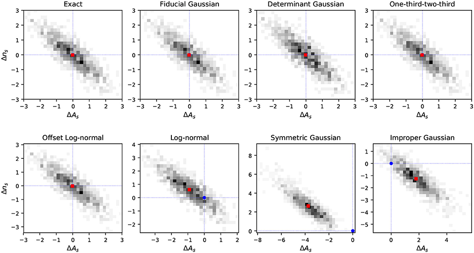
Figure 1. 2D histograms of the biases on the parameters expectation values estimated from 1000 simulated full-sky maps of CMB temperature plus noise. As described in more detail in the text, the biases are computed with respect to the input parameter values and normalized to the 1σ uncertainty associated to the parameter, $\Delta p=(\hat{p}-p^{in})/{\sigma }_p$, where p can be either A_s or n_s. The blue circle indicates a null bias, while the red square is the center of the distribution. Note that for the cases plotted in the first row the two almost completely overlap.

Consistently with what has been presented in section 3.2, we find that the Log-Normal together with the symmetric and improper Gaussian approximations show significant bias in the recovered parameters. The bias is due to the fact that the approximations fail in capturing the correct skewness of the likelihood function. The symmetric Gaussian approximation appears to be the one with the largest associated bias and the wider distribution. For this approximation the covariance is proportional to the measured power spectrum squared, ${Ĉ}_{\ell }^2$. This means that the uncertainties turn out to be larger than they should be if Ĉ_ℓ fluctuates upward with respect to the input fiducial model, and viceversa if Ĉ_ℓ has a downward fluctuation. As a consequence, upward fluctuations are given less weight in the likelihood than downward fluctuations. This translates into an overall downward bias on the amplitude of the power spectrum, and thus on A_s, as it can be easily seen in Figure 1. The one-third-two-third approximation is a good match to the exact likelihood at third order, as shown in Figure 2, and it appears to provide unbiased parameter results. This is the likelihood approximation adopted by the WMAP team for the analysis of the temperature anisotropies on small angular scales [39]. The offset-lognormal also results in unbiased constraints (bottom left panel in Figure 1), as expected since the offset a_TT = −1/4 has been chosen to match the exact likelihood up to third order in the expansion, see section 3.2. Also the fiducial and determinant Gaussian approximations provide unbiased cosmological parameter estimates, despite having a wrong shape at each single ℓ with respect to the exact likelihood. This is because at each particular ℓ the shape of the likelihood can randomly be wrong upwards or downwards with respect to the true C_ℓ (see Figure 2), so when integrating over the entire range of multipoles there is negligible bias left. An obvious advantage of the fiducial Gaussian approximation with respect to the determinant Gaussian is that the covariance matrix can be pre-computed, inverted, and then kept fixed while sampling the parameter space. Aside from speeding up the computations, this makes it easier to account for additional uncertainties, non-Gaussianities and correlations in the data by simply adding extra terms in the pre-computed covariance matrix. The fiducial Gaussian approximation is the one used for the official small-scale likelihood analysis of the Planck data [40], and it has also been adopted for the cosmological analysis of data collected by the ground-based experiments ACT [97] and SPT [98]. Note, however, that this approximation works well if the models we are trying to fit are smooth, and if the fiducial model used to build the covariance matrix is sufficiently close to the true model. In the tests presented here the fiducial model entering the covariance matrix actually coincides with the true model, i.e., the power spectrum from which the simulated maps are generated. Obviously, in this case the covariance matrix is an optimal description of the simulated data. However, when dealing with real data we are not in the same fortunate position, since the true power spectrum underlying the observed sky is unknown and is exactly what we indent to estimate. In a real situation we can only deduce a fiducial model for the covariance at the best of our knowledge from both theory and observations. We can also try to improve the accuracy of a first guess covariance matrix by iterating the cosmological parameter extraction a few times, upgrading the covariance matrix at each iteration. Note that, we did not include the Hamimeche-Lewis approximation in the tests, the reason being that on the full-sky it coincides with the exact likelihood.

FIGURE 2

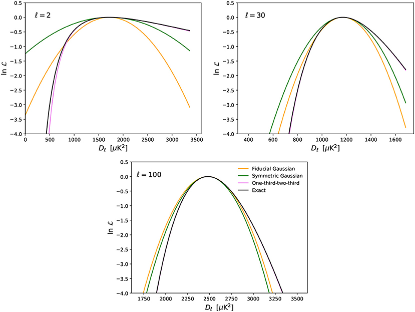
Figure 2. Comparison of some of the likelihood approximations for different multipole regimes, as marked in the plots, where the x-axis corresponds to D_ℓ = ℓ(ℓ + 1)C_ℓ/(2π).

In order to perform an even more stringent validation of the likelihood approximations, we can estimate the bias of the mean of the recovered parameters from all the simulations: $(\langle \hat{p}\rangle -p^{in})/({\sigma }_p/\sqrt{N_{sims}})$, where the shift with respect to the input is normalized by the standard deviation of the mean, and N_sims = 1000. This test confirms, at high-significance level, that Log-Normal, symmetric and improper Gaussian approximations provide biased results, while the other approximations are unbiased. For the latter likelihood approximations we find that the estimated uncertainties on parameters, σ_p, agree with those derived from the exact likelihood at the sub-precent level. Furthermore, we find that the standard deviation of the values of $(\hat{p}-p^{in})/{\sigma }_p$ is consistent to 1, with a precision well within the accuracy allowed by the finite number of simulations, i.e., $1/\sqrt{2N_{sims}}=0.022$. This means that the uncertainties estimated from the bayesian analysis, σ_p, are consistent with the scatter of the parameters of the simulations.

7.1.2. Temperature and Polarization Joint Results

For the fiducial Gaussian approximation, we repeat the test of parameters recovery from the full-sky simulated maps also including the polarization power spectra. As we have already commented, this likelihood approximation works well provided that the fiducial power spectra used to build the covariance matrix are close enough to the true power spectra. In order to investigate the impact on the final parameters of misestimating the covariance matrix, we change the fiducial model entering the likelihood with power spectra at the edge of the grid of models introduced above. These power spectra correspond to parameters more than 10σ away from the input parameters. As expected, results show some sensitivity to the choice of the model, however not for the bias, but rather for the parameters marginal error bars. In fact, using the “wrong” covariance matrix leaves parameters estimates unbiased. This can be noticed in Figure 3, where we show the biases on A_s and n_s estimated from the simulations, both using the covariance matrix with the correct fiducial model and the one with the modified model. The latter covariance matrix, however, does not match exactly the signal in the simulated dataset, and as a consequence the estimated 1σ marginal error bars on the cosmological parameters do not agree with the standard deviation from the simulations, showing a ~ 15% mismatch.

FIGURE 3

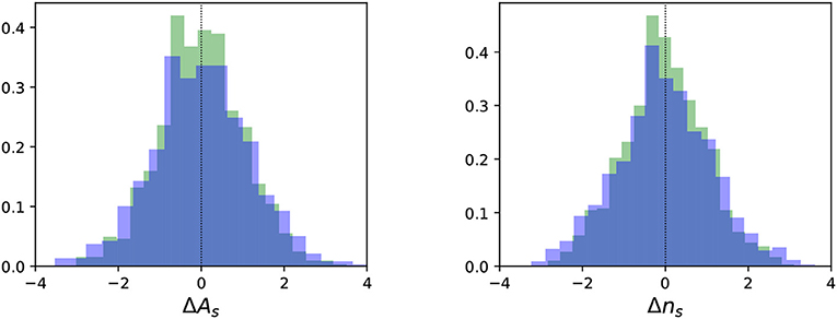
Figure 3. Histograms of the biases for the parameters expectation values estimated from the power spectra of 1000 simulated full-sky maps of CMB temperature and polarization, plus white isotropic noise. Biases are defined with respect to the input parameter values and normalized to the 1σ uncertainty on the parameter, $\Delta p=(\hat{p}-p^{in})/{\sigma }_p$, where p can be either A_s or n_s. We adopt the fiducial Gaussian likelihood approximation, in green the case in which the fiducial model entering the covariance matrix matches the input model of the simulations, whereas in blue a case in which the two models differ as explained in the text.

7.2. Small-Scale Regime—Cut-Sky Tests

We repeat the above analysis introducing some further level of complication, specifically we assume to work with partial-sky and anisotropic noise data. We generate noise simulations which have a different level of noise variance for each pixel, thus mimicking the effect of a realistic scan strategy for which some regions of the sky are observed more often than others. To the simulated CMB plus noise maps we then apply a galactic sky mask, that removes the region of the galactic plane where the emission of foregrounds is expected to dominate over the CMB signal. For the sake of this test, we focus on temperature alone and we use a galactic mask that leaves for the analysis 73% of sky. The mask has been apodised with a Gaussian taper that smooths sharp edges and, thus, it helps in localizing the mask power in multipole space. The angular power spectra of the cut-sky maps are extracted using an estimator that corrects for the loss of modes due to the masking and which is based on the pseudo-C_ℓ formalism. For completeness the estimator is described in Appendix B. The covariance matrix associated to these power spectra has been estimated using the analytic approximation given in Efstathiou [27], and assuming as fiducial model the same model from which the simulations have been generated.

For the parameters recovery test on the cut-sky we explore the fiducial gaussian and Hamimeche-Lewis likelihood approximations. The latter in the single field regime reduces to:

$\begin{array}{ll}-2\ln ℒ\simeq {\displaystyle \sum _{\ell {\ell }^{\prime }}[}g({\hat{C}}_{\ell }/C_{\ell })C_{f\ell }]{[M_f^{-1}]}_{\ell {\ell }^{\prime }}[g({\hat{C}}_{{\ell }^{\prime }}/C_{{\ell }^{\prime }})C_{f{\ell }^{\prime }}],& (69)\end{array}$

where the function g(x) has been introduced in Equation (51), and ${\left[M\right]}_f{}_{\ell {\ell }^{\prime }}$ is the covariance matrix of the Ĉ_ℓ evaluated for C_fℓ.

Following the same procedure described in the previous subsection, we fit for the cosmological parameters A_s and n_s. We find that, also under more realistic conditions, the recovered parameters for the fiducial gaussian are unbiased well within the precision allowed by the finite number of Monte Carlo simulations. For the Hamimeche-Lewis approximation, instead, we detect a small bias at the level of 20 and 11% of the sigma on the parameter for A_s and n_s respectively, see Figure 4. For both likelihood approximations, however, we find that the parameters marginal errors from the bayesian analysis are consistent with the standard deviation of the simulations, and thus they appear to be a good description of the true uncertainties.

FIGURE 4

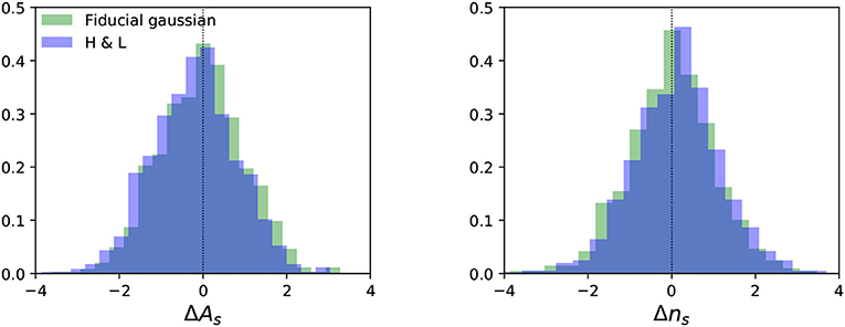
Figure 4. Histograms of the biases for the parameters expectation values estimated from the power spectra of 1000 simulated partial-sky maps of CMB temperature anisotropies plus anisotropic noise. Biases are defined analogously to Figure 3. We compare results from the fiducial gaussian and the Hamimeche-Lewis likelihood approximations.

Despite the small average bias, the Hamimeche-Lewis approximation is expected to be more robust against the choice of the fiducial model entering the likelihood, see [32]. In order to verify this point, when computing the likelihood and the covariance matrix of the Ĉ_ℓ, we use a fiducial model C_fℓ that corresponds to parameters about 10σ away from those used to generate the simulations. As we have already shown in the previous subsection, in this case the fiducial Gaussian approximation provides still unbiased results, but the bayesian error bars on the parameters are not a good description of the true uncertainties. They differ from the standard deviation of the parameters from the simulations by about 14% on A_s and 11% on n_s, respectively. On the contrary, estimates with the Hamimeche-Lewis approximation still show the same level of average bias, but the uncertainties on the parameters are better characterized and they are in agreement with the standard deviation from the simulations.

Furthermore, since it is customary to assess the goodness of the parameters fit with the chi-square statistics, we may use the value of the likelihood at the best-fit to define an effective chi-square as ${\chi }_{eff}^2=\text{min}\left[-2\text{ln}{L}(\theta |{Ĉ}_{\ell })\right]$. If we now compare the values we get for each likelihood approximation when simply varying the fiducial model, we find $\Delta {\chi }_{eff}^2$ of order a few hundreds for the fiducial Gaussian approximation, and $\Delta {\chi }_{eff}^2$ of a few tens for the Hamimeche-Lewis. As a consequence, trying to assess the goodness of the fit with the latter likelihood can surely provide more stable results, regardless of the fiducial model. However, it is worth stressing that in the present test we used a C_fℓ that deviates significantly from the model behind the simulations, had we chosen a model closer to the simulations, also the fiducial Gaussian approximation would have provided sensible results. For further discussion of this topic refer to the appendix B of Hamimeche and Lewis [32].

7.3. Large-Scale Regime

In this subsection, we focus on the comparison of different likelihood approaches devoted to the analysis of large-scale CMB data. We limit the comparison of large-scale likelihoods to the polarization signal only, since this is the main target of future CMB missions [99]. Moreover, the standard approaches used in temperature, i.e., pixel-based and Blackwell-Rao (see section 5.2) likelihoods, have been extensively characterized and validated by the Planck Collaboration, see e.g., [37, 38].

We consider three approaches: pixel-based (see section 5.1), HL (see Equations 49a-54a) and simulation-based (see section 5.3) likelihood. As we did for the small scale regime, we show whether adopting a particular likelihood approximation when estimating cosmological parameters may introduce a bias, either in the recovered values of the parameters or on their associated error bars.

We start by generating a set of 1000 maps of the CMB sky drawn as Gaussian random realizations of a single fiducial power spectrum corresponding to a set of known cosmological parameters. The full sky maps are generated on a N_side = 16 HEALPix grid, which roughly corresponds to a resolution of 3.7 degrees, smoothed with a cosine window function [38, 100]. To each of these maps we add a realization of white isotropic noise corresponding to ${\sigma }_N=0.01\mu K^2$ on a pixel at our resolution. We choose this particular noise level since it is small but not completely negligible with respect to the typical peak-to-peak CMB signal in a model with a reionization optical depth τ = 0.055, that would be roughly ~ 0.5μK. We do not include foreground and systematics effect residuals in our simulations. We process the maps through a QML code computing the auto spectra of all our simulations.

To test the performance of the likelihood approximations, for simplicity, we only fit the reionization optical depth τ parameter keeping fixed the overall amplitude of the perturbations as parametrized through A_sexp(−2τ). For each realization we compute the mean value of τ. The histograms of the τ values, recovered using the three different approximations, are shown in Figure 5. The distributions all show a bias smaller than 5% of σ(τ), perfectly compatible with the resolution of 1000 simulations, (i.e., $1/\sqrt{1000}~3\%$). The Hamimeche-Lewis likelihood and the simulation-based likelihood, both built on the QML estimates, perform similarly and are substantially unbiased. Likewise, the pixel-based likelihood results unbiased as it should, as also already extensively demonstrated by both the WMAP [101] and Planck [37] collaborations. The comparison with the pixel-based likelihood allows also to validate the width of the distributions for the other two likelihood approximations, which are compatible with the pixel based at the 2% level, within the resolution of the Montecarlo (i.e., $1/\sqrt{2\times 1000}~2\%$).

FIGURE 5

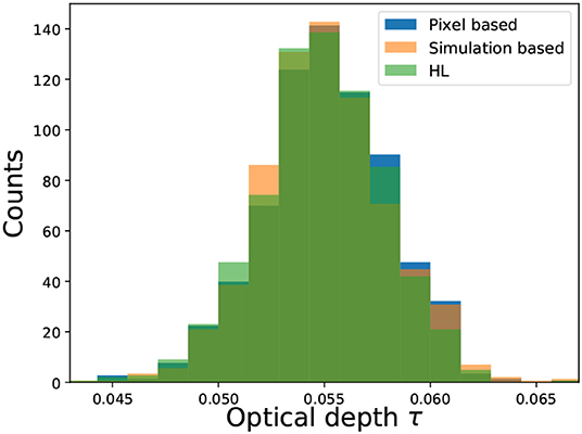
Figure 5. Histograms of the recovered values of τ for the three likelihoods considered: pixel based (blue), simulation based (orange), and Hamimeche-Lewis (green).

8. Conclusions

CMB science is nowadays a mature yet still flourishing branch of physics. The ultimate results from the Planck satellite and from large-aperture ground-based experiments (ACT and SPT) fully characterize the CMB temperature field with great accuracy up to very small angular scales, where the contaminations from Galactic and extra-Galactic foreground emissions become dominant. In addition, they have just scratched the surface of the rich information contained in the CMB polarization fields, also the target of small-aperture telescopes (BICEP/Keck, POLARBEAR/Simons Array, SPIDER). A large number of upcoming CMB surveys (Simons Observatory, CMB-S4, LiteBIRD) will continue the journey toward the understanding of the early phases of our Universe and its subsequent evolution.

In the highly sophisticated process that aims to efficiently compress the information contained in the raw observed data into maps, spectra, and eventually constraints on cosmological parameters, a key ingredient is the likelihood function ${L}(\text{d}|\theta )$, i.e., the probability of observing a certain data collection d given a certain model θ (see section A). In the context of CMB analysis, d can be either a CMB map or CMB spectra, while θ can be the set of cosmological parameters describing the cosmological model under scrutiny. In the simple case of full-sky observations, in absence of foreground contaminations and late-time-Universe effects on the CMB distribution, an exact form of the likelihood function in both real (multivariate Gaussian) and harmonic space (Wishart distribution) can be easily derived, see section 2. Complications arising from realistic observations and data analysis, such as complicated noise properties, foreground obscuration, limited sky coverage, computational costs, etc, may spoil the assumptions on which the derivation of the exact likelihood functions mentioned above is based, or may limit the actual evaluation of the exact functions. Therefore, realistic analysis employ appropriate approximations of the exact likelihood functions, see sections 3, 5. The choice of the likelihood depends on multiple factors, such as sky-fraction retained, data resolution, computational costs, signal-to-noise properties. For example, it may (and actually did) happen that a certain likelihood approximation could work for a certain experiment given its sensitivity, and yet it could turn out to provide biased results for another, more sensitive experiment.

In this review, we have summarized the basics of CMB statistics (section 2) that lead to the definition of the exact likelihoods in real and harmonic space. Then, we have moved to the descriptions of the most common likelihood approximations employed by various CMB collaborations. For the sake of simplicity, we have separated the approximations better suited to the analysis of small angular scales (higher harmonic multipoles) in section 3 and those that better represent the data at large angular scales (lower multipoles) in section 5. Although we have mostly assumed an idealized scenario of isotropic instrumental noise, Gaussian beam, unlensed CMB spectra, and absence of foreground for pedagogical reasons, we have commented about the impact of realistic deviations from the aforementioned scenario, in such a way that the reader is aware of their existence and of the extensive effort devoted to their mitigation. In particular, non-trivial modifications to the primary CMB statistics induced by the gravitational lensing of CMB photons by the evolving large-scale structure in the Universe have been discussed in section 4. In section 6, we have briefly discussed the main foreground contaminants in the microwave sky and mentioned methods of component separation aimed to disentangle the cosmological signal from Galactic and extra-Galactic emissions.

In order to provide concrete examples of the different performance of various likelihood methods, we have reported results of the comparison between different likelihood approximations in section 7. In particular, we have tested the property of the likelihood function to be unbiased, i.e., to produce a posterior distribution of cosmological parameters that matches the true cosmology (the input values, in the case of simulated data) both in terms of the mean and of the variance of the distribution. Again, we have distinguished between approximations at small scales (section 7.1) and at large scales (section 7.3).

In Appendix, the interested reader can find more details about some basics of statistical inference (section A) and about the most common methods adopted to estimate CMB power spectra in the (realistic) cut-sky regime (section B).

The aim of this review is to bring together and summarize a large amount of information related to a crucial aspect of CMB data analysis. The final scope is to provide a handy, yet self-consistent document to those who are approaching the field and those who are interested in learning some basic aspects of the field, and help them to navigate the vast literature produced over the past decades on these topics. If you have gone so far in your reading, we hope to have reached, at least partly, our goal.

Author Contributions

All the authors contributed in a relevant way to the development and finalization of the manuscript. The ordering of the authors (two tiers, alphabetic order in each tier) reflects the relative contribution, with authors within each tier having contributed equally.

Conflict of Interest

The authors declare that the research was conducted in the absence of any commercial or financial relationships that could be construed as a potential conflict of interest.

Acknowledgments

The authors would like to thank D. Poletti for useful discussions. We acknowledge support from the ASI grant 2016-24-H.0 COSMOS Attività di studio per la comunità scientifica di cosmologia. MG acknowledges support by Argonne National Laboratory (ANL). This work was supported by the U.S. Department of Energy, Office of Science, under contract number DE-AC02-06CH11357. ML and MM acknowledge support from INFN through the InDark and Gruppo IV fundings. MM is supported by the program for young researchers Rita Levi Montalcini year 2015. LS acknowledges support from the ERC-StG ClustersXCosmo grant agreement 716762, and from the postdoctoral grant from Centre National d'Études Spatiales (CNES). LC received funding from the European Union's Horizon 2020 research and innovation programme under grant number 776282.

Supplementary Material

The Supplementary Material for this article can be found online at: https://www.frontiersin.org/articles/10.3389/fphy.2020.00015/full#supplementary-material

Footnotes

1. ^The base ΛCDM parameters are: the angular size of the sound horizon at recombination θ_*, the amplitude A_S and tilt n_s of the spectrum of primordial scalar perturbations, the reionization optical depth τ, the energy density in baryonic matter ${\Omega }_b{h}^2$ and in cold dark matter ${\Omega }_c{h}^2$.

2. ^Constraints derived in the context of minimal extensions of the standard ΛCDM model.

3. ^In this section, “observed” stands for what would be observed in the idealized situation considered here, i.e., negligible instrumental noise and absence of contaminants of any kind. A more proper term would be “realized,” but in this context we avoid to use it as we reserve it for simulated CMB sky signals.

4. ^One of the assumptions is that the matrix of the estimators Ĉ_ℓ is positive definite. This assumption may break up at large scales.

5. ^In passing from Equations (49a) to (49b), we have made use of the properties of the trace[] operator.

6. ^Using the invariance of Tr[A] under diagonalization of A, one has that

$\begin{array}{ll}\text{Trace}[g(D_{\ell })]=\text{Trace}[Ug(D_{\ell })U^T]& (\mathrm{52a})\end{array}$

$\begin{array}{ll}=\text{Trace}[C_{\ell }^{-1/2}{\hat{C}}_{\ell }{C}_{\ell }^{-1/2}]& (\mathrm{52b})\end{array}$

$\begin{array}{ll}=\text{Trace}[C_{f\ell }^{-1/2}{C}_{f\ell }^{1/2}\left(C_{\ell }^{-1/2}{\hat{C}}_{\ell }{C}_{\ell }^{-1/2}\right)C_{f\ell }^{1/2}{C}_{f\ell }^{-1/2}]& (\mathrm{52c})\end{array}$

$\begin{array}{ll}=\text{Trace}[C_{f\ell }^{-1/2}{C}_{g\ell }{C}_{f\ell }^{-1/2}]& (\mathrm{52d})\end{array}$

7. ^We are dropping the BB part of the distribution, as we have seen that the full Wishart in full-sky is separable into a T − E and B component. For the B component, all considerations in the single-field regime apply.

8. ^If $a_{\ell m}^i=s_{\ell m}^i+n_{\ell }^i$, with noise nⁱ uncorrelated for any map i = 1, …, nmaps and signal sⁱ, then $\sum _m\left|a_{\ell m}^i{(a_{\ell m}^j)}^{*}\right|=\sum _m|s_{\ell m}^i{(s_{\ell m}^j)}^{*}+n_{\ell m}^i{(n_{\ell m}^j)}^{*}|=(2\ell +1){Ĉ}_{\ell }^{ij}$.

9. ^The unperturbed line of sight in the Born approximation.

10. ^Small enough that the convergence and shear components of the deflection field can be assumed constant in the patch.

11. ^The signal in each pixel is the average over the signal at each point within the surface area of the pixel Ω_p, f_p = ∫dΩw_pf(Ω), where w_p = 1/Ω_p is the weight inside the pixel and zero otherwise. The harmonic transform of the weight w_p is the pixel window function. Including the full dependence of the window function on m, ℓ can be computationally demanding. However, if the size of the pixel is small compared to the angular resolution of the experiment, the m-dependence can be neglected and the m-averaged window function w_ℓ can be defined. The power spectra computed from the pixelised maps $C_{\ell }^p$ are related to the unpixelised spectra C_ℓ via $C_{\ell }^p=w_{\ell }^2{C}_{\ell }$.

12. ^Component separation methods and related references can be accessed at the following url: https://lambda.gsfc.nasa.gov/toolbox/tb_comp_separation.cfm

13. ^Roughly speaking, the resolution identifies the level of the discretization (i.e., the number of pixels). The beam smoothing simulates the angular resolution of the experiment, and exponentially suppresses the scales below the beam width. Note that the beam width is larger than the size of the pixel.

References

1. Hu W, Dodelson S. Cosmic microwave background anisotropies. Annu Rev Astron Astrophys. (2002) 40:171–216. doi: 10.1146/annurev.astro.40.060401.093926

CrossRef Full Text | Google Scholar

2. Kolb EW, Turner MS. The early Universe. Front Phys. (1990) 69:1–547.

Google Scholar

3. Aghanim N, Akrami Y, Ashdown M, Aumont J, Baccigalupi C, Ballardini M, et al. Planck 2018 results. VI. Cosmological parameters. arXiv [Preprint]. arXiv:1807.06209 (2018).

Google Scholar

4. Hinshaw G, Larson D, Komatsu E, Spergel DN, Bennett CL, Dunkley J, et al. Nine-year Wilkinson Microwave Anisotropy Probe (WMAP) observations: cosmological parameter results. Astrophys J. (2012) 208:19. doi: 10.1088/0067-0049/208/2/19

CrossRef Full Text | Google Scholar

5. Bennett CL, Banday A, Gorski KM, Hinshaw G, Jackson P, Keegstra P, et al. Four year COBE DMR cosmic microwave background observations: maps and basic results. Astrophys J. (1996) 464:L1–4. doi: 10.1086/310075

CrossRef Full Text | Google Scholar

6. Fraisse AA, Ade PAR, Amiri M, Benton SJ, Bock JJ, Bond JR, et al. SPIDER: probing the early Universe with a suborbital polarimeter. J Cosmol Astropart Phys. (2013) 1304:047. doi: 10.1088/1475-7516/2013/04/047

CrossRef Full Text | Google Scholar

7. Aboobaker AM, Ade P, Araujo D, Aubin F, Baccigalupi C, Bao C, et al. The EBEX balloon-borne experiment? Optics, receiver, and polarimetry. Astrophys J Suppl. (2018) 239:7. doi: 10.3847/1538-4365/aae434

CrossRef Full Text | Google Scholar

8. de Bernardis P, Ade PAR, Bock JJ, Bond JR, Borrill J, Boscaleri A, et al. A flat universe from high resolution maps of the cosmic microwave background radiation. Nature. (2000) 404:955–9. doi: 10.1038/35010035

PubMed Abstract | CrossRef Full Text | Google Scholar

9. Louis T, Grace E, Hasselfield M, Lungu M, Maurin L, Addison GE, et al. The atacama cosmology telescope: two-season ACTPol spectra and parameters. J Cosmol Astropart Phys. (2017) 1706:031. doi: 10.1088/1475-7516/2017/06/031

CrossRef Full Text | Google Scholar

10. Henning JW, Sayre JT, Reichardt CL, Ade PAR, Anderson AJ, Austermann JE, et al. Measurements of the temperature and E-mode polarization of the CMB from 500 square degrees of SPTpol data. Astrophys J. (2018) 852:97. doi: 10.3847/1538-4357/aa9ff4

CrossRef Full Text | Google Scholar

11. Ade PAR, Ahmed Z, Aikin RW, Alexander KD, Barkats D, Benton SJ, et al. BICEP2 / Keck Array x: constraints on primordial gravitational waves using Planck, WMAP, and New BICEP2/Keck observations through the 2015 season. Phys Rev Lett. (2018) 121:221301. doi: 10.1103/PhysRevLett.121.221301

CrossRef Full Text | Google Scholar

12. Ade PAR, Aguilar M, Akiba Y, Arnold K, Baccigalupi C, Barron D, et al. A measurement of the cosmic microwave background B-Mode polarization power spectrum at sub-degree scales from 2 years of POLARBEAR Data. Astrophys J. (2017) 848:121. doi: 10.3847/1538-4357/aa8e9f

CrossRef Full Text | Google Scholar

13. Essinger-Hileman T, Ali A, Amiri M, Appel JW, Araujo D, Bennett CL, et al. CLASS: the cosmology large angular scale surveyor. Proc SPIE Int Soc Opt Eng. (2014) 9153:91531I. doi: 10.1117/12.2056701

CrossRef Full Text | Google Scholar

14. Akrami Y, Arroja F, Ashdown M, Aumont J, Baccigalupi C, Ballardini M, et al. Planck 2018 results. I. Overview and the cosmological legacy of Planck arXiv [Preprint]. arXiv:1807.06205 (2018).

Google Scholar

15. Henderson SW, Allison R, Austermann J, Baildon T, Battaglia N, Beall JA, et al. Advanced ACTPol cryogenic detector arrays and readout. J Low Temp Phys. (2016) 184:772–9. doi: 10.1007/s10909-016-1575-z

CrossRef Full Text | Google Scholar

16. Benson BA, Ade PAR, Ahmed Z, Allen SW, Arnold K, Austermann JE, et al. SPT-3G: a next-generation cosmic microwave background polarization experiment on the south pole telescope. Proc SPIE Int Soc Opt Eng. (2014) 9153:91531P. doi: 10.1117/12.2057305

CrossRef Full Text | Google Scholar

17. Suzuki A, Ade PAR, Akiba Y, Aleman C, Arnold K, Baccigalupi C, et al. The POLARBEAR-2 and the simons array experiment. J Low Temp Phys. (2016) 184:805–10. doi: 10.1007/s10909-015-1425-4

CrossRef Full Text | Google Scholar

18. Bergman AS, Ade PAR, Akers S, Amiri M, Austermann JA, Beall JA, et al. 280 GHz focal plane unit design and characterization for the spider-2 suborbital polarimeter. J Low Temp Phys. (2018) 193:1075–84. doi: 10.1007/s10909-018-2065-2

CrossRef Full Text | Google Scholar

19. Abazajian KN, Adshead P, Ahmed Z, Allen SW, Alonso D, Arnold KS, et al. CMB-S4 Science Book, 1st Edn. arXiv [Preprint]. arXiv:1610.02743 (2016).

Google Scholar

20. Ade PAR, Aguirre J, Ahmed Z, Aiola S, Ali A, Alonso D, et al. The simons observatory: science goals and forecasts. J Cosmol Astropart Phys. (2019) 1902:056. doi: 10.1088/1475-7516/2019/02/056

CrossRef Full Text | Google Scholar

21. Matsumura T, Akiba Y, Borrill J, Chinone Y, Dobbs M, Fuke H, et al. Mission design of LiteBIRD. J Low Temp Phys. (2014) 176:733. doi: 10.1007/s10909-013-0996-1

CrossRef Full Text | Google Scholar

22. Delabrouille J, de Bernardis P, Bouchet FR, Achùcarro A, Ade PAR, Allison R, et al. Exploring cosmic origins with CORE: survey requirements and mission design. J Cosmol Astropart Phys. (2018) 1804:014. doi: 10.1088/1475-7516/2018/04/014

CrossRef Full Text | Google Scholar

23. Hanany S, Bennett C, Dodelson S, Page L, Bartlett J, Battaglia N, et al. PICO: probe of inflation and cosmic origins. arXiv [Preprint]. arXiv:1902.10541 (2019).

Google Scholar

24. Penzias AA, Wilson RW. A Measurement of excess antenna temperature at 4080-Mc/s. Astrophys J. (1965) 142:419–21. doi: 10.1086/148307

CrossRef Full Text | Google Scholar

25. Akrami Y, Arroja F, Ashdown M, Aumont J, Baccigalupi C, Ballardini M, et al. Planck 2018 results. IX. Constraints on primordial non-Gaussianity arXiv [Preprint]. arXiv:1905.05697 (2019).

Google Scholar

26. Zaldarriaga M, Seljak U. An all sky analysis of polarization in the microwave background. Phys Rev D. (1997) 55:1830–40. doi: 10.1103/PhysRevD.55.1830

CrossRef Full Text | Google Scholar

27. Efstathiou G. Myths and truths concerning estimation of power spectra Mon Not R Astron Soc. (2004) 349:603. doi: 10.1111/j.1365-2966.2004.07530.x

CrossRef Full Text | Google Scholar

28. Zaldarriaga M. The polarization of the cosmic microwave background. arXiv:astro-ph/0305272 (2003).

PubMed Abstract | Google Scholar

29. Percival WJ, Brown ML. Likelihood methods for the combined analysis of CMB temperature and polarisation power spectra Mon Not R Astron Soc. (2006) 372:1104. doi: 10.1111/j.1365-2966.2006.10910.x

CrossRef Full Text | Google Scholar

30. Tegmark M, de Oliveira-Costa A. How to measure CMB polarization power spectra without losing information. Phys Rev D. (2001) 64:063001. doi: 10.1103/PhysRevD.64.063001

CrossRef Full Text | Google Scholar

31. Upham RE, Whittaker L, Brown ML. Exact joint likelihood of pseudo-C_ℓ estimates from correlated Gaussian cosmological fields. Mon Not R Astron Soc. (2020) 491:3165. doi: 10.1093/mnras/stz3225

CrossRef Full Text | Google Scholar

32. Hamimeche S, Lewis A. “Likelihood analysis of CMB temperature and polarization power spectra. Phys Rev D. (2008) 77:103013. doi: 10.1103/PhysRevD.77.103013

CrossRef Full Text | Google Scholar

33. Bond JR, Jaffe AH, Knox LE. Radical compression of cosmic microwave background data. Astrophys J. (2000) 533:19. doi: 10.1086/308625

CrossRef Full Text | Google Scholar

34. Smith S, Challinor A, Rocha G. What can be learned from the lensed cosmic microwave background B-mode polarization power spectrum? Phys Rev D. (2006) 73:023517. doi: 10.1103/PhysRevD.73.023517

CrossRef Full Text | Google Scholar

35. Lewis A, Challinor A, Turok N. Analysis of CMB polarization on an incomplete sky. Phys Rev D. (2001) 65:023505. doi: 10.1103/PhysRevD.65.023505

CrossRef Full Text | Google Scholar

36. Slosar A, Seljak U, Makarov A. Exact likelihood evaluations and foreground marginalization in low resolution WMAP data. Phys Rev D. (2004) 69:123003. doi: 10.1103/PhysRevD.69.123003

CrossRef Full Text | Google Scholar

37. Aghanim N, Arnaud M, Ashdown M, Aumont J, Baccigalupi C, Banday AJ, et al. Planck 2015 results. XI. CMB power spectra, likelihoods, and robustness of parameters. Astron Astrophys. (2016) 594:A11. doi: 10.1051/0004-6361/201526926

CrossRef Full Text | Google Scholar

38. Aghanim N, Akrami Y, Ashdown M, Aumont J, Baccigalupi C, Ballardini M, et al. Planck 2018 results. V. CMB power spectra and likelihoods. arXiv [Preprint]. arXiv:1907.12875 (2019).

Google Scholar

39. Verde L, Peiris HV, Spergel DN, Nolta M, Bennett CL, Halpern M, et al. First year Wilkinson Microwave Anisotropy Probe (WMAP) observations: parameter estimation methodology. Astrophys J Suppl. (2003) 148:195. doi: 10.1086/377335

CrossRef Full Text | Google Scholar

40. Ade PAR, Aghanim N, Armitage-Caplan C, Arnaud M, Ashdown M, Atrio-Barandela F, et al. Planck 2013 results. XV. CMB power spectra and likelihood. Astron Astrophys. (2014) 571:A15. doi: 10.1051/0004-6361/201321573

CrossRef Full Text | Google Scholar

41. Lewis A, Challinor A. Weak gravitational lensing of the CMB. Phys Rept. (2006) 429:1–65. doi: 10.1016/j.physrep.2006.03.002

CrossRef Full Text | Google Scholar

42. Ade PAR, Aghanim N, Armitage-Caplan C, Arnaud M, Ashdown M, Atrio-Barandela F, et al. Planck 2013 results. XVII. Gravitational lensing by large-scale structure. Astron Astrophys. (2014) 571:A17. doi: 10.1051/0004-6361/201321543

CrossRef Full Text | Google Scholar

43. Okamoto T, Hu W. CMB lensing reconstruction on the full sky. Phys Rev D. (2003) 67:083002. doi: 10.1103/PhysRevD.67.083002

CrossRef Full Text | Google Scholar

44. Hu W, Okamoto T. Mass reconstruction with cmb polarization. Astrophys J. (2002) 574:566–74. doi: 10.1086/341110

CrossRef Full Text | Google Scholar

45. Aghanim N, Akrami Y, Ashdown M, Aumont J, Baccigalupi C, Ballardini M, et al. Planck 2018 results. VIII. Gravitational lensing. arXiv [Preprint]. arXiv:1807.06210 (2018).

Google Scholar

46. Sherwin BD, van Engelen A, Sehgal N, Madhavacheril M, Addison GE, Aiola S, et al. Two-season Atacama Cosmology Telescope polarimeter lensing power spectrum. Phys Rev D. (2017) 95:123529. doi: 10.1103/PhysRevD.95.123529

CrossRef Full Text | Google Scholar

47. Omori Y, Chown R, Simard G, Story KT, Aylor K, Baxter EJ, et al. A 2500 deg² CMB lensing map from combined south pole telescope and planck data. Astrophys J. (2017) 849:124. doi: 10.3847/1538-4357/aa8d1d

CrossRef Full Text | Google Scholar

48. Ade PAR, Akiba Y, Anthony AE, Arnold K, Barron D, Boettger D, et al. Evidence for gravitational lensing of the cosmic microwave background polarization from cross-correlation with the cosmic infrared background. Phys Rev Lett. (2014) 112:131302. doi: 10.1103/PhysRevLett.112.131302

PubMed Abstract | CrossRef Full Text | Google Scholar

49. Challinor A, Allison R, Carron J, Errard J, Feeney S, Kitching T, et al. Exploring cosmic origins with CORE: gravitational lensing of the CMB. J Cosmol Astropart Phys. (2018) 1804:018. doi: 10.1088/1475-7516/2018/04/018

CrossRef Full Text | Google Scholar

50. Schmittfull MM, Challinor A, Hanson D, Lewis A. Joint analysis of CMB temperature and lensing-reconstruction power spectra. Phys Rev D. (2013) 88:063012. doi: 10.1103/PhysRevD.88.063012

CrossRef Full Text | Google Scholar

51. Lewis A, Challinor A, Lasenby A. Efficient computation of CMB anisotropies in closed FRW models. Astrophys J. (2000) 538:473–6. doi: 10.1086/309179

CrossRef Full Text

52. Lesgourgues J. The Cosmic Linear Anisotropy Solving System (CLASS) I: overview. arXiv [Preprint]. arXiv:1104.2932 (2011).

Google Scholar

53. Benoit-Lévy A, Smith KM, Hu W. Non-Gaussian structure of the lensed CMB power spectra covariance matrix. Phys Rev D. (2012) 86:123008. doi: 10.1103/PhysRevD.86.123008

CrossRef Full Text | Google Scholar

54. Lewis A. Lensed CMB simulation and parameter estimation. Phys Rev D. (2005) 71:083008. doi: 10.1103/PhysRevD.71.083008

CrossRef Full Text | Google Scholar

55. Motloch P, Hu W. Lens covariance effects on likelihood analyses of CMB power spectra. Phys Rev D. (2017) 96:103517. doi: 10.1103/PhysRevD.96.103517

CrossRef Full Text | Google Scholar

56. Motloch P, Hu W, Benoit-Lévy A. CMB lens sample covariance and consistency relations. Phys Rev D. (2017) 95:043518. doi: 10.1103/PhysRevD.95.043518

CrossRef Full Text | Google Scholar

57. Green D, Meyers J, van Engelen A. CMB delensing beyond the B modes. J Cosmol Astropart Phys. (2017) 1712:005. doi: 10.1088/1475-7516/2017/12/005

CrossRef Full Text | Google Scholar

58. Vanneste S, Henrot-Versillé S, Louis T, Tristram M. Quadratic estimator for CMB cross-correlation. Phys Rev D. (2018) 98:103526. doi: 10.1103/PhysRevD.98.103526

CrossRef Full Text | Google Scholar

59. Aghanim N, Ashdown M, Aumont J, Baccigalupi C, Ballardini M, Banday AJ, et al. Planck intermediate results. XLVI. Reduction of large-scale systematic effects in HFI polarization maps and estimation of the reionization optical depth. Astron Astrophys. (2016) 596:A107. doi: 10.1051/0004-6361/201628890

CrossRef Full Text | Google Scholar

60. Gorski KM, Hivon E, Banday AJ, Wandelt BD, Hansen FK, Reinecke M, et al. HEALPix - A Framework for high resolution discretization, and fast analysis of data distributed on the sphere. Astrophys J. (2005) 622:759–71. doi: 10.1086/427976

CrossRef Full Text | Google Scholar

61. Hinshaw G, Nolta MR, Bennett CL, Bean R, Dore O, Greason MR, et al. Three-year Wilkinson Microwave Anisotropy Probe (WMAP) observations: temperature analysis. Astrophys J Suppl. (2007) 170:288. doi: 10.1086/513698

CrossRef Full Text | Google Scholar

62. Eriksen HK, O'Dwyer IJ, Jewell JB, Wandelt BD, Larson DL, Gorski KM, et al. Power spectrum estimation from high-resolution maps by Gibbs sampling. Astrophys J Suppl. (2004) 155:227–41. doi: 10.1086/425219

CrossRef Full Text | Google Scholar

63. Jewell J, Levin S, Anderson CH. Application of Monte Carlo algorithms to the Bayesian analysis of the cosmic microwave background. Astrophys J. (2004) 609:1–14. doi: 10.1086/383515

CrossRef Full Text | Google Scholar

64. Wandelt BD, Larson DL, Lakshminarayanan A. Global, exact cosmic microwave background data analysis using Gibbs sampling. Phys Rev D. (2004) 70:083511. doi: 10.1103/PhysRevD.70.083511

CrossRef Full Text | Google Scholar

65. Eriksen HK, Jewell JB, Dickinson C, Banday AJ, Gorski KM, Lawrence CR. Joint Bayesian component separation and CMB power spectrum estimation. Astrophys J. (2008) 676:10–32. doi: 10.1086/525277

CrossRef Full Text | Google Scholar

66. Chu M, Eriksen HK, Knox L, Gorski KM, Jewell JB, Larson DL, et al. Cosmological parameter constraints as derived from the Wilkinson Microwave Anisotropy Probe data via Gibbs sampling and the Blackwell-Rao estimator. Phys Rev D. (2005) 71:103002. doi: 10.1103/PhysRevD.71.103002

CrossRef Full Text | Google Scholar

67. Rudjord O, Groeneboom NE, Eriksen HK, Huey G, Gorski KM, Jewell JB. CMB likelihood approximation by a Gaussianized Blackwell-Rao estimator. Astrophys J. (2009) 692:1669–77. doi: 10.1088/0004-637X/692/2/1669

CrossRef Full Text | Google Scholar

68. Akrami Y, Ashdown M, Aumont J, Baccigalupi C, Ballardini M, Banday AJ, et al. Planck 2018 results. IV. Diffuse component separation. arXiv [Preprint]. arXiv:1807.06208 (2018).

Google Scholar

69. Ade PAR, Aghanim N, Alves MIR, Arnaud M, Ashdown M, Aumont J, et al. Planck 2015 results. XXV. Diffuse low-frequency Galactic foregrounds. Astron Astrophys. (2016) 594:A25. doi: 10.1051/0004-6361/201526803

CrossRef Full Text | Google Scholar

70. Ade PAR, Aghanim N, Armitage-Caplan C, Arnaud M, Ashdown M, Atrio-Barandela F, et al. Planck 2013 results. XII. Diffuse component separation. Astron Astrophys. (2014) 571:A12. doi: 10.1051/0004-6361/201321580

CrossRef Full Text | Google Scholar

71. Larson D, Dunkley J, Hinshaw G, Komatsu E, Nolta MR, Bennett CL, et al. Seven-Year Wilkinson Microwave Anisotropy Probe (WMAP) observations: power spectra and WMAP-derived parameters. Astrophys J Suppl. (2011) 192:16. doi: 10.1088/0067-0049/192/2/16

CrossRef Full Text | Google Scholar

72. Pritchard JK, Seielstad MT, Perez-Lezaun A, Feldman MW. Population growth of human y chromosomes: a study of y chromosome microsatellites. Mol Biol Evol. (1999) 16:1791–8.

PubMed Abstract | Google Scholar

73. Beaumont MA, Zhang W, Balding DJ. Approximate bayesian computation in population genetics. Genetics. (2002) 162:2025–35.

PubMed Abstract | Google Scholar

74. Marjoram P, Molitor J, Plagnol V, Tavaré S. Markov chain monte carlo without likelihoods. Proc Natl Acad Sci USA. (2003) 100:15324–8. doi: 10.1073/pnas.0306899100

PubMed Abstract | CrossRef Full Text | Google Scholar

75. Sisson SA, Fan Y, Tanaka MM. Sequential monte carlo without likelihoods. Proc Natl Acad Sci USA. (2007) 104:1760–5. doi: 10.1073/pnas.0607208104

PubMed Abstract | CrossRef Full Text | Google Scholar

76. Toni T, Welch D, Strelkowa N, Ipsen A, Stumpf MP. Approximate bayesian computation scheme for parameter inference and model selection in dynamical systems. J R Soc Interface. (2009) 6:187–202. doi: 10.1098/rsif.2008.0172

PubMed Abstract | CrossRef Full Text | Google Scholar

77. Beaumont MA, Cornuet JM, Marin JM, Robert CP. Adaptive approximate bayesian computation. Biometrika. (2009) 96:983–90. doi: 10.1093/biomet/asp052

CrossRef Full Text | Google Scholar

78. McKinley T, Cook AR, Deardon R. Inference in epidemic models without likelihoods. Int J Biostat. 5:24. doi: 10.2202/1557-4679.1171

CrossRef Full Text | Google Scholar

79. Beaumont MA. Approximate bayesian computation in evolution and ecology. Annu Rev Ecol Evol Syst. (2010) 41:379–406. doi: 10.1146/annurev-ecolsys-102209-144621

CrossRef Full Text | Google Scholar

80. Liepe J, Kirk P, Filippi S, Toni T, Barnes CP, Stumpf MP. A framework for parameter estimation and model selection from experimental data in systems biology using approximate bayesian computation. Nat Protoc.(2014) 9:439–56. doi: 10.1038/nprot.2014.025

PubMed Abstract | CrossRef Full Text | Google Scholar

81. Turner BM, Van Zandt T. A tutorial on approximate bayesian computation. J Math Psychol. (2012) 56:69–85. doi: 10.1016/j.jmp.2012.02.005

CrossRef Full Text | Google Scholar

82. Akeret J, Refregier A, Amara A, Seehars S, Hasner C, Approximate Bayesian computation for forward modeling in cosmology. J Cosmol Astropart Phys. (2015) 1508:043. doi: 10.1088/1475-7516/2015/08/043

CrossRef Full Text | Google Scholar

83. Alsing J, Wandelt B. Nuisance hardened data compression for fast likelihood-free inference. Mon Not R Astron Soc. (2019) 488:5093. doi: 10.1093/mnras/stz1900

CrossRef Full Text | Google Scholar

84. Alsing J, Charnock T, Feeney S, Wandelt B. Fast likelihood-free cosmology with neural density estimators and active learning. Mon Not R Astron Soc. (2019) 488:4440. doi: 10.1093/mnras/stz1960

CrossRef Full Text | Google Scholar

85. Leclercq F. Bayesian optimization for likelihood-free cosmological inference. Phys Rev D. (2018) 98:063511. doi: 10.1103/PhysRevD.98.063511

CrossRef Full Text | Google Scholar

86. Alsing J, Wandelt B, Feeney S. Massive optimal data compression and density estimation for scalable, likelihood-free inference in cosmology. Mon Not R Astron Soc. (2018) 477:2874. doi: 10.1093/mnras/sty819

CrossRef Full Text | Google Scholar

87. Delabrouille J, Betoule M, Melin JB, Miville-Deschenes MA, Gonzalez-Nuevo J, Le Jeune M, et al. The pre-launch Planck Sky Model: a model of sky emission at submillimetre to centimetre wavelengths. Astron. Astrophys. (2013) 553:A96. doi: 10.1051/0004-6361/201220019

CrossRef Full Text | Google Scholar

88. Sehgal N, Bode P, Das S, Hernandez-Monteagudo C, Huffenberger K, Lin Y, et al. Simulations of the microwave sky. Astrophys J. (2010) 709:920–36. doi: 10.1088/0004-637X/709/2/920

CrossRef Full Text | Google Scholar

89. Ichiki K. CMB foreground: a concise review. Prog Theor Exp Phys. 6:2014. doi: 10.1093/ptep/ptu065

CrossRef Full Text | Google Scholar

90. Takakura S, Aguilar M, Akiba Y, Arnold K, Baccigalupi C, Barron D, et al. Performance of a continuously rotating half-wave plate on the POLARBEAR telescope J Cosmol Astropart Phys. (2017) 1705:008. doi: 10.1088/1475-7516/2017/05/008

CrossRef Full Text | Google Scholar

91. Leach SM, Cardoso JF, Baccigalupi C, Barreiro RB, Betoule M, Bobin J, et al. Component separation methods for the Planck mission. Astron Astrophys. (2008) 491:597–615. doi: 10.1051/0004-6361:200810116

CrossRef Full Text | Google Scholar

92. Bennett CL, Smoot GF, Hinshaw G, Wright EL, Kogut A, de Amici G, et al. Preliminary separation of galactic and cosmic microwave emission for the COBE Differential Microwave Radiometer. Astrophys J. (1992) 396:L7–12. doi: 10.1086/186505

CrossRef Full Text | Google Scholar

93. Fernandez-Cobos R, Vielva P, Barreiro RB, Martinez-Gonzalez E. Multi-resolution internal template cleaning: an application to the Wilkinson Microwave Anisotropy Probe 7-yr polarization data. Mon Not R Astron Soc. (2012) 420:2162. doi: 10.1111/j.1365-2966.2011.20182.x

CrossRef Full Text | Google Scholar

94. Delabrouille J, Cardoso JF, Jeune ML, Betoule M, Fay G, Guilloux F. A full sky, low foreground, high resolution CMB map from WMAP. Astron Astrophys. (2009) 493:835. doi: 10.1051/0004-6361:200810514

CrossRef Full Text | Google Scholar

95. Eriksen HK, Dickinson C, Lawrence CR, Baccigalupi C, Banday AJ, Gorski KM, et al. CMB component separation by parameter estimation. Astrophys J. (2006) 641:665–82. doi: 10.1086/500499

CrossRef Full Text | Google Scholar

96. Cardoso JF, Martin M, Delabrouille J, Betoule M, Patanchon G. Component separation with flexible models. Application to the separation of astrophysical emissions. arXiv [Preprint]. arXiv:0803.1814 (2008).

Google Scholar

97. Dunkley J, Calabrese E, Sievers J, Addison GE, Battaglia N, Battistelli ES, et al. The Atacama Cosmology Telescope: likelihood for small-scale CMB data” J Cosmol Astropart Phys. (2013) 1307:025. doi: 10.1088/1475-7516/2013/07/025

CrossRef Full Text | Google Scholar

98. Keisler R, Reichardt CL, Aird KA, Benson BA, Bleem LE, Carlstrom JE, et al. A measurement of the damping tail of the cosmic microwave background power spectrum with the south pole telescope. Astrophys J. (2011) 743:28. doi: 10.1088/0004-637X/743/1/28

CrossRef Full Text | Google Scholar

99. Suzuki A, Ade PAR, Akiba Y, Alonso D, Arnold K, Aumont J, et al. The LiteBIRD Satellite Mission - Sub-Kelvin Instrument. J Low Temp Phys. (2018) 193:1048–56. doi: 10.1007/s10909-018-1947-7

CrossRef Full Text | Google Scholar

100. Benabed K, Cardoso JF, Prunet S, Hivon E. TEASING: a fast and accurate approximation for the low multipole likelihood of the Cosmic Microwave Background temperature. Mon Not R Astron Soc. (2009) 400:219. doi: 10.1111/j.1365-2966.2009.15202.x

CrossRef Full Text | Google Scholar

101. Page L, Hinshaw G, Komatsu E, Nolta MR, Spergel DN, Bennett CL, et al. Three year Wilkinson Microwave Anisotropy Probe (WMAP) observations: polarization analysis. Astrophys J Suppl. (2007) 170:335. doi: 10.1086/513699

CrossRef Full Text | Google Scholar

102. Hivon E, Gorski KM, Netterfield CB, Crill BP, Prunet S, Hansen F. Master of the cosmic microwave background anisotropy power spectrum: a fast method for statistical analysis of large and complex cosmic microwave background data sets. Astrophys J. (2002) 567:2. doi: 10.1086/338126

CrossRef Full Text | Google Scholar

103. Wandelt BD, Hivon E, Gorski KM. The pseudo-C_ℓ method: cosmic microwave background anisotropy power spectrum statistics for high precision cosmology. Phys Rev D. (2001) 64:083003. doi: 10.1103/PhysRevD.64.083003

CrossRef Full Text | Google Scholar

104. Brown ML, Castro PG, Taylor AN. Cosmic microwave background temperature and polarization pseudo-C_ℓ estimators and covariances. Mon Not R Astron Soc. (2005) 360:4. doi: 10.1111/j.1365-2966.2005.09111.x

CrossRef Full Text | Google Scholar

105. Bunn EF, Zaldarriaga M, Tegmark M, de Oliveira-Costa A. E/B decomposition of finite pixelized CMB maps. Phys Rev D. (2003) 67:023501. doi: 10.1103/PhysRevD.67.023501

CrossRef Full Text | Google Scholar

106. Challinor A, Chon G. Error analysis of quadratic power spectrum estimates for CMB polarization: sampling covariance. Mon Not R Astron Soc. (2005) 360:509. doi: 10.1111/j.1365-2966.2005.09076.x

CrossRef Full Text | Google Scholar

107. Grain J, Tristram M, Stompor R. Polarized CMB power spectrum estimation using the pure pseudo-cross-spectrum approach. Phys Rev D. (2009) 79:123515. doi: 10.1103/PhysRevD.79.123515

CrossRef Full Text | Google Scholar

108. Smith KM, Zaldarriaga M. A general solution to the E-B mixing problem. Phys Rev D. (2007) 76:043001. doi: 10.1103/PhysRevD.76.043001

CrossRef Full Text | Google Scholar

109. Smith KM. Pseudo-C_ℓ estimators which do not mix E and B modes. Phys Rev D. (2006) 74:083002. doi: 10.1103/PhysRevD.74.083002

CrossRef Full Text | Google Scholar

110. Zaldarriaga M. Fluctuations in the cosmic microwave background. arXiv:astro-ph/9806122 (1998).

Google Scholar

111. Tegmark M. How to measure CMB power spectra without losing information. Phys Rev D. (1997)55:5895. doi: 10.1103/PhysRevD.55.5895

CrossRef Full Text | Google Scholar

112. Bond JR, Jaffe AH, Knox L. Estimating the power spectrum of the cosmic microwave background. Phys Rev D. (1998) 57:2117. doi: 10.1103/PhysRevD.57.2117

CrossRef Full Text | Google Scholar