Numerical Treatment of Time-Fractional Klein–Gordon Equation Using Redefined Extended Cubic B-Spline Functions

1. Introduction

The subject of fractional-order differential equations has attracted considerable interest due to its applications in a wide range of fields, such as traffic flow, earthquakes and other physical phenomena, signal processing, finance, control theory, fractional dynamics, and mathematical modeling [1–10]. In recent years, the analytical and numerical study of fractional-order differential equations has become a dynamic area of research. Several numerical and analytical techniques have been developed to handle these types of equations [11–22]. There are a number of different definitions of fractional-order derivatives, with different applications. An excellent overview can be found in the works [23–31]. This article is concerned with the following time-fractional non-linear Klein–Gordon equation (KGE):

$\begin{array}{ll}\frac{{\partial }^{\alpha }}{\partial t^{\alpha }}v(x,t)+\rho \frac{{\partial }^2}{\partial x^2}v(x,t)+{\rho }_{1}v(x,t)+{\rho }_2{v}^{\sigma }(x,t)=f(x,t),0<x\le L,t_0<t\le T,& (1)\end{array}$

$\begin{array}{ll}v(x,t_0)={\phi }_1(x),v_t(x,t_0)={\phi }_2(x),& (2)\end{array}$

$\begin{array}{ll}v(0,t)={\phi }_3(t),v(L,t)={\phi }_4(t),& (3)\end{array}$

where $\frac{{\partial }^{\alpha }}{\partial t^{\alpha }}$ represents the Caputo fractional time derivative, v = v(x, t) denotes the displacement of the wave at (x, t), α ∈ (1, 2] is the fractional order of the time derivative, f(x, t) is the source term, ρ, ρ₁ and ρ₂ are real numbers, and σ = 2 or 3.

The fractional KGE plays a significant role in quantum mechanics, the study of solitons, and condensed matter physics. Many approaches have been adopted to solve equations of Klein/sine–Gordon type efficiently, including the Adomian decomposition method, the variational iteration method [32–34], and the homotopy analysis method [35]; see also the references cited in these works. Jafari et al. proposed using fractional B-splines for approximate solution of fractional differential equations [36]. In Vong and Wang [37, 38] space compact difference schemes were applied to one- and two-dimensional time-fractional Klein–Gordon-type equations, and stability and convergence of the proposed numerical approaches were established with the aid of an energy method. In Dehghan et al. [39] the authors used a meshless method based on radial basis functions to develop an unconditionally stable numerical scheme for fractional Klein/sine–Gordon equations. The Adomian decomposition method and an iterative method were applied in Jafari [40] to solve Klein–Gordon-type equations involving fractional time derivatives. A fully spectral approach was employed in Chen et al. [41] that uses finite differences for time discretization and Legendre spectral approximation in the spatial direction to construct numerical solutions of non-linear partial differential equations involving fractional derivatives. A sinc–Chebyshev collocation method (SCCM) was developed in Nagy [42] for numerical treatment of the time-fractional non-linear KGE. Recently, in Kanwal et al. [43], Genocchi polynomials were employed together with the Ritz–Galerkin scheme to solve fractional KGEs and diffusion wave equations. A linearized second-order scheme was introduced in Lyu and Vong [44] to solve non-linear time-fractional Klein–Gordon-type equations. Later on, in Doha et al. [45], a space–time spectral approximation was proposed for solving non-linear variable-order fractional Klein/sine–Gordon differential equations.

In this article we propose using redefined extended cubic B-spline (RECBS) functions for numerical solution of the time-fractional KGE. RECBS functions are basically a generalization of typical cubic B-spline functions that involve a free parameter which provides the flexibility to fine-tune the solution curve. We employ the usual finite central difference approach to discretize the Caputo fractional time derivative and use RECBS functions for spatial integration.

This article is organized as follows. The Caputo definition of fractional time derivative and the finite difference formulation for temporal discretization are reviewed in section 2; this section also includes a brief introduction to extended cubic B-spline and RECBS functions and their applications to space discretization. The stability analysis of the proposed algorithm is presented in section 3, and the description of theoretical convergence is given in section 4. The approximate results are reported and discussed in section 5. Finally, concluding remarks are given in section 6.

2. Description of Numerical Technique

2.1. Time Discretization

Let the time domain [0, T] be divided into R subintervals of equal length $\Delta t=\frac{T}{R}$ with endpoints 0 = t₀ < t₁ < ⋯ < t_R = T, where t_r = rΔt and r = 0:1:R. We first discretize the Caputo fractional derivative at t = t_r+1 as [46]

$\begin{array}{l}\frac{{\partial }^{\alpha }v(x,t_{r+1})}{\partial t^{\alpha }}=\frac{1}{\Gamma (2-\alpha )}{\displaystyle \underset{0}{\overset{t_k}{\int }}}\frac{{\partial }^{2}v(x,w)}{\partial w^2}{(t_{r+1}-w)}^{-\alpha +1}dw\\ (1<\alpha \le 2)\\ =\frac{1}{\Gamma (2-\alpha )}{\displaystyle \sum _{k=0}^r}{\displaystyle \underset{t_k}{\overset{t_{k+1}}{\int }}}\frac{{\partial }^{2}v(x,w)}{\partial w^2}{(t_{r+1}-w)}^{-\alpha +1}dw.\\ =\frac{1}{\Gamma (2-\alpha )}{\displaystyle \sum _{k=0}^r}\frac{v(x,t_{k+1})-2v(x,t_k)+v(x,t_{k-1})}{\Delta t^2}\\ \begin{array}{l}{\displaystyle \underset{t_k}{\overset{t_{k+1}}{\int }}}{(t_{r+1}-w)}^{-\alpha +1}dw+l_{\Delta t}^{r+1}\end{array}\\ \begin{array}{l}=\frac{1}{\Gamma (2-\alpha )}{\displaystyle \sum _{k=0}^r}\frac{v(x,t_{k+1})-2v(x,t_k)+v(x,t_{k-1})}{\Delta t^2}\\ {\displaystyle \underset{t_{r-k}}{\overset{t_{r-k+1}}{\int }}}{(ϵ)}^{-\alpha +1}dϵ+l_{\Delta t}^{r+1}\\ =\frac{1}{\Gamma (2-\alpha )}{\displaystyle \sum _{k=0}^r}\frac{v(x,t_{r-k+1})-2v(x,t_{r-k})+v(x,t_{r-k-1})}{\Delta t^2}\\ {\displaystyle \underset{t_k}{\overset{t_{k+1}}{\int }}}{(ϵ)}^{-\alpha +1}dϵ+l_{\Delta t}^{r+1}\\ =\frac{1}{\Gamma (3-\alpha )}{\displaystyle \sum _{k=0}^r}\frac{v(x,t_{r-k+1})-2v(x,t_{r-k})+v(x,t_{r-k-1})}{\Delta t^{\alpha }}\\ ({(k+1)}^{2-\alpha }-k^{2-\alpha })+l_{\Delta t}^{r+1}\\ =\frac{1}{\Gamma (3-\alpha )}{\displaystyle \sum _{k=0}^r}{p}_k\frac{\begin{array}{c}v(x,t_{r-k+1})-2v(x,t_{r-k})+\\ v(x,t_{r-k-1})\end{array}}{\Delta t^{\alpha }}+l_{\Delta t}^{r+1},\end{array}& (4)\end{array}$

where $p_k={(k+1)}^{2-\alpha }-k^{2-\alpha }$, ϵ = (t_r+1 − w), and $l_{\Delta t}^{r+1}$ is the truncation error. The truncation error is bounded, i.e.,

$\begin{array}{ll}\left|l_{\Delta t}^{r+1}\right|\le \psi {(\Delta t)}^{2-\alpha },& (5)\end{array}$

where ψ is a constant. The coefficients p_k in (4) possess the following attributes:

• the p_k's are non-negative for k = 0, 1, 2, …, r;

• 1 = p₀ > p₁ > p₂ > p₃ > ⋯ > p_n, and p_n → 0 as n → ∞;

• $(2p_0-p_1)+\sum _{k=1}^{r-1}(-p_{k+1}+2p_k-p_{k-1})+(2p_r-p_{r-1})-p_r=1$.

Substituting Equation (4) into Equation (1), we get

$\begin{array}{l}\frac{1}{\Gamma (3-\alpha ){(\Delta t)}^{\alpha }}{\displaystyle \sum _{k=0}^r}{p}_k[v(x,t_{r-k+1})-2v(x,t_{r-k})+v(x,t_{r-k-1})]\\ +\rho v_{xx}(x,t)+{\rho }_{1}v(x,t)+{\rho }_2{v}^{\sigma }(x,t)=f(x,t)\\ \begin{array}{l}(r=0,1,2,\dots ,R-1).\end{array}& (6)\end{array}$

Suppose $\beta =\frac{1}{\Gamma (3-\alpha ){(\Delta t)}^{\alpha }}$ and $v(x,t_{r+1})=v^{r+1}$. Applying a θ-weighted scheme, Equation (6) takes the form

$\begin{array}{l}\beta p_0(v^{r+1}-2v^r+v^{r-1})+\beta {\displaystyle \sum _{k=1}^r{p}_k}(v^{r-k+1}-2v^{r-k}+v^{r-k-1})\\ +\theta (\rho v_{xx}^{r+1}\\ +{\rho }_1{v}^{r+1})=f^{r+1}-(1-\theta )(\rho v_{xx}^r+{\rho }_1{v}^r)-{\rho }_2{(v^{\sigma })}^r\\ (r=0,1,2,\dots ,R-1).& (7)\end{array}$

For θ = 1, we obtain the following semi-discretized numerical scheme:

$\begin{array}{l}(\beta p_0+{\rho }_1)v^{r+1}+\rho v_{xx}^{r+1}=2\beta p_0{v}^r+\beta {\displaystyle \sum _{k=1}^r{p}_k}(v^{r-k+1}-2v^{r-k}\\ +v^{r-k-1})-{\rho }_2{(v^{\sigma })}^r-\beta p_0{v}^{r-1}+f^{r+1}(r=0,1,2,\dots ,R-1).& (8)\end{array}$

2.2. Extended Cubic B-Spline Functions

Let the spatial domain [a, b] be partitioned into M parts of equal length $h=\frac{b-a}{M}$ with boundary points a = x₀ < x₁ < ⋯ < x_M = b, where x_m = x₀ + mh for m = 0:1:M. For a sufficiently continuous function v(x, t), there always exists a unique extended cubic B-spline (ECBS) approximation V^*(x, t):

$\begin{array}{ll}{V}^{*}(x,t)={\displaystyle \sum _{m=-1}^{M+1}}{\xi }_m(t)S_m(x,\lambda ),& (9)\end{array}$

where the ξ_m(t) are to be calculated and the fourth-degree ECBS blending functions S_m(x, λ) are defined as [47]

$\begin{array}{ll}{S}_m(x,\lambda )=\frac{1}{24h^4}\{\begin{array}{cc}4h{(x-x_{m-2})}^3(1-\lambda )+3{(x-x_{m-2})}^4\lambda \hfill & \text{if }x\in [x_{m-2},x_{m-1}),\hfill \\ h^4(4-\lambda )+12h^3(x-x_{m-1})+6h^2{(x-x_{m-1})}^2(2+\lambda )\hfill \\ -12h{(x-x_{m-1})}^3-3{(x-x_{m-1})}^4\lambda \hfill & \text{if }x\in [x_{m-1},x_m),\hfill \\ h^4(4-\lambda )-12h^3(x-x_{m+1})-6h^2{(x-x_{m+1})}^2(2+\lambda )\hfill \\ +12h{(x-x_{m+1})}^3+3{(x-x_{m-1})}^4\lambda \hfill & \text{if }x\in [x_m,x_{m+1}),\hfill \\ -4h{(x-x_{m+2})}^3(1-\lambda )-3{(x-x_{m+2})}^4\lambda \hfill & \text{if }x\in [x_{m+1},x_{m+2}),\hfill \\ 0\hfill & \text{otherwise}.\hfill \end{array}\hfill & (10)\end{array}$

Here λ, with −n(n − 2) ≤ λ ≤ 1, is a real number responsible for fine-tuning the curve, and n gives the degree of the ECBS used to generate different forms of ECBS functions. The approximate solution ${(V^{*})}_m^r=V^{*}(x_m,t^r)$ and its first two derivatives with respect to the spatial variable x at the rth time step can be expressed in terms of ξ_m as [48]

$\begin{array}{ll}\{\begin{array}{c}{(V^{*})}_m^r=b_1{\xi }_{m-1}^r+b_2{\xi }_m^r+b_1{\xi }_{m+1}^r,\hfill \\ {(V_x^{*})}_m^r=b_3{\xi }_{m-1}^r-b_3{\xi }_{m+1}^r,\hfill \\ {(V_{xx}^{*})}_m^r=b_4{\xi }_{m-1}^r+b_5{\xi }_m^r+b_4{\xi }_{m+1}^r,\hfill \end{array}\hfill & (11)\end{array}$

where $b_1=\frac{4-\lambda }{24}$, $b_2=\frac{16+2\lambda }{24}$, $b_3=\frac{-1}{2h}$, $b_4=\frac{2+\lambda }{2h^2}$, and $b_5=\frac{-4-2\lambda }{2h^2}$.

2.3. Redefined Extended Cubic B-Spline Functions

In the typical ECBS collocation method, the basis functions S₋₁, S₀, …, S_M+1 do not vanish at the boundaries of the spatial domain when Dirichlet-type end conditions are imposed. Therefore, we need to redefine them so that the resulting set of basis functions will vanish at the boundaries. For this, a weight function Φ(x, t) is introduced to eliminate ξ₋₁ and ξ_M+1 from Equation (9) in the following manner [49]:

$\begin{array}{ll}V(x,t)=\Phi (x,t)+{\displaystyle \sum _{m=0}^M}{\xi }_m(t){\tilde{S}}_m(x,\lambda ),& (12)\end{array}$

where the weight function Φ(x, t) and the redefined ECBS (RECBS) functions are given by

$\begin{array}{ll}\Phi (x,t)=\frac{S_{-1}(x,\lambda )}{S_{-1}(x_0,\lambda )}{\phi }_3(t)+\frac{S_{M+1}(x,\lambda )}{S_{M+1}(x_M,\lambda )}{\phi }_4(t)& (13)\end{array}$

and.

$\begin{array}{ll}\{\begin{array}{cc}{\tilde{S}}_m(x,\lambda )=S_m(x,\lambda )-\frac{S_m(x_0,\lambda )}{S_{-1}(x_0,\lambda )}{S}_{-1}(x,\lambda )\hfill & \text{for }m=0,1,\hfill \\ {\tilde{S}}_m(x,\lambda )=S_m(x,\lambda )\hfill & \text{for }m=2:1:M-2,\hfill \\ {\tilde{S}}_m(x,\lambda )=S_m(x,\lambda )-\frac{S_m(x_M,\lambda )}{S_{M+1}(x_M,\lambda )}{S}_{M+1}(x,\lambda )\hfill & \text{for }m=M-1,M.\hfill \end{array}\hfill & (14)\end{array}$

2.4. Space Discretization

Using Equation (12) in Equation (8) at t = t_r+1, we obtain

$\begin{array}{l}(\beta p_0+{\rho }_1)V^{r+1}+\rho V_{xx}^{r+1}=2\beta p_0{V}^r+\beta {\displaystyle \sum _{k=1}^r{p}_k}(V^{r-k+1}\\ -2V^{r-k}+V^{r-k-1})-{\rho }_2{(V^{\sigma })}^r-\beta p_0{V}^{r-1}+f^{r+1}.& (15)\end{array}$

Discretizing at x = x_j, we get

$\begin{array}{l}(\beta +{\rho }_1)V_j^{r+1}+\rho {(V_{xx})}_j^{r+1}=2\beta V_j^r+\beta {\displaystyle \sum _{k=1}^r{p}_k}(V_j^{r-k+1}-2V_j^{r-k}\\ +V_j^{r-k-1})-{\rho }_2{(V^{\sigma })}_j^r-\beta V_j^{r-1}+f_j^{r+1}(j=0,1,2,\dots ,M).& (16)\end{array}$

Using (12), the last expression takes the form

$\begin{array}{l}(\beta +{\rho }_1)\left[{\Phi }_j^{r+1}+{\displaystyle \sum _{m=0}^M{\xi }_m^{r+1}}{\tilde{S}}_m(x_j,\lambda )\right]+\rho [{({\Phi }_{xx})}_j^{r+1}\\ +{\displaystyle \sum _{m=0}^M{\xi }_m^{r+1}}{\tilde{S}}_m(x_j,\lambda )]\\ =2\beta V_j^r+\beta {\displaystyle \sum _{k=1}^r{p}_k}(V_j^{r-k+1}-2V_j^{r-k}+V_j^{r-k-1})\\ -{\rho }_2{(V^{\sigma })}_j^r-\beta V_j^{r-1}+f_j^{r+1}\\ (j=0,1,2,\dots ,M).& (17)\end{array}$

Consequently, we get the following system of M + 1 equations in M + 1 unknowns:

$\begin{array}{ll}\left(\begin{array}{ccccccc}{a}_1^{*}& \text{}& \text{}& \text{}& \text{}& \text{}& \text{}\\ a_1& a_2& a_1& \text{}& \text{}& \text{}& \text{}\\ \text{}& a_1& a_2& a_1& \text{}& \text{}& \text{}\\ \text{}& \text{}& \ddots & \ddots & \ddots & \text{}& \text{}\\ \text{}& \text{}& \text{}& a_1& a_2& a_1& \text{}\\ \text{}& \text{}& \text{}& \text{}& a_1& a_2& a_1\\ \text{}& \text{}& \text{}& \text{}& \text{}& \text{}& a_1^{*}\end{array}\right)\left(\begin{array}{c}{\xi }_0^{r+1}\\ {\xi }_1^{r+1}\\ ⋮\\ ⋮\\ {\xi }_{M-1}^{r+1}\\ {\xi }_M^{r+1}\end{array}\right)=\left(\begin{array}{c}{y}_0\\ y_1\\ ⋮\\ ⋮\\ y_{M-1}\\ y_M\end{array}\right),& (18)\end{array}$

where

$\begin{array}{l}{a}_1^{*}=\frac{12\rho (\lambda +2)}{h^2(\lambda -4)},a_1=\frac{h^2(\beta +{\rho }_1)(\lambda -4)+12\rho (\lambda +2)}{24h^2},\\ a_2=\frac{h^2(\beta +{\rho }_1)(\lambda +8)-12\rho (\lambda +2)}{12h^2},\\ y_j=2\beta V_j^r+\beta {\displaystyle \sum _{k=1}^r}{p}_k(V_j^{r-k+1}-2V_j^{r-k}+V_j^{r-k-1})\\ -{\rho }_2{(V^{\sigma })}_j^r-\beta V_j^{r-1}+{\text{Ψ}}_j^{r+1},\\ {\text{Ψ}}_j^r=f_j^r-(\beta +{\rho }_1){\Phi }_j^r-\rho {({\Phi }_{xx})}_j^r.\end{array}$

To start the numerical procedure, we use the given initial conditions to obtain the set of equations

$\begin{array}{ll}\{\begin{array}{cc}{(V^{\prime })}_m^0={{\phi }^{\prime }}_1(x_m)\hfill & \text{ for }m=0,\hfill \\ {(V)}_m^0={\phi }_1(x_m)\hfill & \text{ for }m=1:1:M-1,\hfill \\ {(V^{\prime })}_m^0={{\phi }^{\prime }}_1(x_m)\hfill & \text{ for }m=M.\hfill \end{array}\hfill & (19)\end{array}$

The matrix representation of (19) is

$\begin{array}{l}\left(\begin{array}{ccccccc}{b}_1^{*}& b_2^{*}& \text{}& \text{}& \text{}& \text{}& \text{}\\ b_1& b_2& b_1& \text{}& \text{}& \text{}& \text{}\\ \text{}& b_1& b_2& b_1& \text{}& \text{}& \text{}\\ \text{}& \text{}& \ddots & \ddots & \ddots & \text{}& \text{}\\ \text{}& \text{}& \text{}& b_1& b_2& b_1& \text{}\\ \text{}& \text{}& \text{}& \text{}& b_1& b_2& b_1\\ \text{}& \text{}& \text{}& \text{}& \text{}& -b_2^{*}& -b_1^{*}\end{array}\right)\left(\begin{array}{c}{\xi }_0^0\\ {\xi }_1^0\\ ⋮\\ ⋮\\ {\xi }_{M-1}^0\\ {\xi }_M^0\end{array}\right)\\ =\left(\begin{array}{c}{({\phi }_1^{\prime })}_0-{({\Phi }^{\prime })}_0^0\\ {({\phi }_1)}_1-{\Phi }_1^0\\ ⋮\\ ⋮\\ {({\phi }_1)}_{M-1}-{\Phi }_{M-1}^0\\ {({\phi }_1^{\prime })}_M-{({\Phi }^{\prime })}_M^0\end{array}\right),& (20)\end{array}$

where $b_1^{*}=\frac{8+\lambda }{h(4-\lambda )}$ and $b_2^{*}=\frac{1}{h}$. We solve (20) to obtain ${\left[{\xi }_0^0,{\xi }_1^0,\dots ,{\xi }_M^0\right]}^T$. The ξ_j values are then substituted into (12) to get V⁰. Now we can use (18) for r = 0, 1, 2, …, R − 1. However, for r = 0 the term involving V⁻¹ appears in Equation (18). This issue is resolved by using the following substitution derived from the velocity condition given in (2):

$\begin{array}{l}{V}^{-1}=V^0-\Delta t{\varphi }_2(x).\end{array}$

3. Stability Analysis

We use the Fourier method to study the stability of the proposed numerical method. Let ${\epsilon }_m^r$ and ${\tilde{\epsilon }}_m^r$ denote, respectively, the exact and approximate growth factors of the Fourier modes. The error, ${\varrho }_m^r$, is given by

$\begin{array}{ll}{\varrho }_m^r={\epsilon }_m^r-{\tilde{\epsilon }}_m^r,m=1:1:M-1,r=0:1:R,& (21)\end{array}$

where ${\varrho }^r={\left[{\epsilon }_1^r,{\epsilon }_2^r,\dots ,{\epsilon }_{M-1}^r\right]}^T$.

For the sake of simplicity, we shall investigate the stability of the proposed scheme with f = 0. The equation for the round-off error is derived from Equations (8) and (21) as

$\begin{array}{l}(\beta b_1+{\rho }_1{b}_1+\rho b_4){\varrho }_{m-1}^{r+1}+(\beta b_2+{\rho }_1{b}_2+\rho b_5){\varrho }_m^{r+1}\\ +(\beta b_1+{\rho }_1{b}_1+\rho b_4){\varrho }_{m+1}^{r+1}\\ =2\beta (b_1{\varrho }_{m-1}^r+b_2{\varrho }_m^r+b_1{\varrho }_{m+1}^r)-\beta (b_1{\varrho }_{m-1}^{r-1}+b_2{\varrho }_m^{r-1}\\ +b_1{\varrho }_{m+1}^{r-1})\\ -\beta {\displaystyle \sum _{k=1}^r{p}_k}{\displaystyle \left[b_1\right({\varrho }_{m-1}^{r-k+1}-2{\varrho }_{m-1}^{r-k}+{\varrho }_{m-1}^{r-k-1})}\\ +b_2({\varrho }_m^{r-k+1}-2{\varrho }_m^{r-k}+{\varrho }_m^{r-k-1})\\ {\displaystyle +b_1({\varrho }_{m+1}^{r-k+1}-2{\varrho }_{m+1}^{r-k}+{\varrho }_{m+1}^{r-k-1})].}& (22)\end{array}$

The error equation satisfies the end conditions

$\begin{array}{ll}{\varrho }_m^0={\phi }_1(x_m),m=1:1:M,& (23)\end{array}$

and

$\begin{array}{ll}{\varrho }_0^r={\phi }_3(t_r),{\varrho }_M^r={\phi }_4(t_r),r=0:1:R.& (24)\end{array}$

We define the grid function as

$\begin{array}{ll}{\varrho }^r=\{\begin{array}{cc}{\varrho }_m^r\hfill & \text{if }{x}_m-\frac{h}{2}<x\le x_m+\frac{h}{2},\text{ for }m=1:1:M-1,\hfill \\ 0\hfill & \text{if }a\le x\le \frac{2a+h}{2}\text{or}\frac{2b-h}{2}\le x\le b.\hfill \end{array}\hfill & (25)\end{array}$

Now, ϱ^r(x) can be written in the form of a Fourier series as follows:

$\begin{array}{ll}{\varrho }^r(x)={\displaystyle \sum _{r=-\infty }^{\infty }}{\epsilon }_r(n)e^{\frac{2\pi \iota nx}{b-a}},r=1:1:R,& (26)\end{array}$

where

$\begin{array}{ll}{\epsilon }_r(n)=\frac{1}{b-a}{\displaystyle {\int }_a^b}{\varrho }^r(x)e^{\frac{-2\pi \iota nx}{b-a}}dx.& (27)\end{array}$

Taking the ‖·‖₂ norm, we get

$\begin{array}{l}\Vert {\varrho }^r{\Vert }_2={\left({\displaystyle \sum _{n=1}^{R-1}}h|{\varrho }_n^r{|}^2\right)}^{\frac{1}{2}}\\ ={\left({\displaystyle {\int }_a^{a+\frac{h}{2}}}|{\varrho }^r{|}^{2}dx+{\displaystyle \sum _{n=1}^{R-1}}{\displaystyle {\int }_{x_n-\frac{h}{2}}^{x_n+\frac{h}{2}}}|{\varrho }^r{|}^{2}dx+{\displaystyle {\int }_{b-\frac{h}{2}}^b}|{\varrho }^r{|}^{2}dx\right)}^{\frac{1}{2}}\\ ={\left({\displaystyle {\int }_a^b}|{\varrho }^r{|}^{2}dx\right)}^{\frac{1}{2}}.\end{array}$

From Parseval's equality we have ${\int }_a^b|{\varrho }^r(n){|}^{2}dx={\sum }_{-\infty }^{\infty }|{\epsilon }_n(m){|}^2$, so the above expression can be written as

$\begin{array}{ll}\begin{array}{l}\Vert {\varrho }^r{\Vert }^{22}={\displaystyle \sum _{r=-\infty }^{\infty }|{\epsilon }_r(n){|}^2.}\hfill \end{array}& (28)\end{array}$

Next, we consider the solution in terms of Fourier series,

$\begin{array}{ll}{\varrho }_k^r={\epsilon }_r{e}^{\iota \nu kh},& (29)\end{array}$

where $\iota =\sqrt{-1}$ and $\nu =\frac{2\pi n}{b-a}$. Using Equation (29) in Equation (22) and then dividing by e^iνkh gives

$\begin{array}{l}(\beta b_1+{\rho }_1{b}_1+\rho b_4){\epsilon }_{r+1}{e}^{-\iota \nu h}+(\beta b_2+{\rho }_1{b}_2+\rho b_5){\epsilon }_{r+1}\\ +(\beta b_1+{\rho }_1{b}_1+\rho b_4){\epsilon }_{r+1}{e}^{\iota \nu h}\\ =2\beta (b_1{\epsilon }_r{e}^{-\iota \nu h}+b_2{\epsilon }_r+b_1{\epsilon }_r{e}^{i\nu h})-\beta (b_1{\epsilon }_{r-1}{e}^{-\iota \nu h}\\ +b_2{\epsilon }_{r-1}+b_1{\epsilon }_{r-1}{e}^{i\nu h})\\ -\beta {\displaystyle \sum _{k=1}^r{p}_k}{\displaystyle [b_1({\epsilon }_{r-k+1}{e}^{-\iota \nu h}-2{\epsilon }_{r-k}+{\epsilon }_{r-k-1}{e}^{\iota \nu h})}\\ +b_2({\epsilon }_{r-k+1}-2{\epsilon }_{r-k}+{\epsilon }_{r-k-1})\\ +b_1({\epsilon }_{r-k+1}{e}^{-\iota \nu h}-2{\epsilon }_{r-k}{e}^{\iota \nu h}+{\epsilon }_{r-k-1}{e}^{\iota \nu h})].& (30)\end{array}$

We know that e^iνh + e^−iνh = 2 cos(νh), so after collecting like terms, the following useful relation is obtained:

$\begin{array}{ll}{\epsilon }_{r+1}=\frac{1}{\eta }[2{\epsilon }_r-{\epsilon }_{r-1}-{\displaystyle \sum _{k=1}^r}{p}_k({\epsilon }_{r-k+1}-2(b_1+b_2){\epsilon }_{r-k}+{\epsilon }_{r-k-1})],& (31)\end{array}$

where $\eta =1+\frac{\rho 1}{\beta }+\frac{12\rho (2+\nu ){\text{sin}}^2(\nu h/2)}{\beta h^2\left\{-6+(4-\nu ){\text{sin}}^2(\nu h/2)\right\}}$. Now it is obvious that η ≥ 1 for ν > −2.

Lemma 3.1. Let ε_r be the solution of Equation (31). Then |ε_r| ≤ |ε₀| for r = 0:1:R.

Proof: For r = 0 in (31), we have

$\begin{array}{l}\left|{\epsilon }_1\right|=\frac{1}{\eta }\left|{\epsilon }_0\right|\le \left|{\epsilon }_0\right|\text{ for }\eta \ge 1.\end{array}$

Suppose that the result is true for r = 1:1:R. Then, from Equation (31) we get

$\begin{array}{l}|{\epsilon }_{r+1}|\le \frac{1}{\eta }|{\epsilon }_r|-\frac{1}{\eta }{\displaystyle \sum _{k=1}^r}{p}_k(|{\epsilon }_{r-k+1}|-2|{\epsilon }_{r-k}|+|{\epsilon }_{r-k-1}|)\\ \le \frac{1}{\eta }|{\epsilon }_0|-\frac{1}{\eta }|{\epsilon }_0|-{\displaystyle \sum _{k=1}^r}{p}_k(|{\epsilon }_0|-|{\epsilon }_0|)\\ \le |{\epsilon }_0|.\end{array}$

Theorem 1. The implic it collocation technique presented in Equation (13) is unconditionally stable.

Proof: Using Lemma (3.1) and Equation (28), we obtain

$\begin{array}{l}\Vert {\varrho }^r{\Vert }_2\le |{\varrho }^0{|}_2,r=0:1:R.\end{array}$

4. Convergence of the Scheme

To investigate the convergence of the proposed scheme, we follow the approach in Khalid et al. [50]. Before proceeding, we state the following useful theorems [51, 52].

Theorem 2. Let Π = {a = x₀, x₁, …, x_M = b} be a partition of [a, b] with x_m = mh for m = 0, …, M, and let v ∈ C⁴[a, b] and f ∈ C²[a, b]. Suppose $\tilde{V}$(x, t) is the spline that interpolates the solution curve of this problem at the knots x_m ∈ Π. Then there exist constants Ϝ_m, not depending on h, such that

$\begin{array}{ll}\Vert {\xi }^j(v(x,t)-\tilde{V}(x,t)){\Vert }_{\infty }\le {Ϝ}_j{h}^{4-j}\forall t\ge 0,j=0,1,2.& (32)\end{array}$

Lemma 4.1. The extended B-splines in (10) satisfy the inequality

$\begin{array}{ll}{\displaystyle \sum _{m=0}^M}\left|S_m(x,\lambda )\right|\le 1.75for0\le x\le 1.& (33)\end{array}$

Proof: By the triangle inequality we have

$\begin{array}{l}\left|{\displaystyle \sum _{m=0}^M}{S}_m(x,\lambda )\right|\le {\displaystyle \sum _{m=0}^M}|S_m(x,\lambda )|.\end{array}$

For any knot x_m, we have

$\begin{array}{l}{\displaystyle \sum _{m=0}^M}|S_m(x,\lambda )|=|S_{m-1}(x_m,\lambda )|+|S_m(x_m,\lambda )|\\ +|S_{m+1}(x_m,\lambda )|=1<\frac{7}{4}.\end{array}$

From (11) we obtain

$\begin{array}{llllllll}\hfill S_m(x_m,\lambda )=\frac{1}{12}(8+\lambda ),& \hfill S_{m-1}(x_{m-1},\lambda )=\frac{1}{12}(8+\lambda ),& \hfill & & \hfill & & & \\ \hfill S_{m+1}(x_m,\lambda )=\frac{1}{24}(4-\lambda ),& \hfill S_{m-2}(x_{m-1},\lambda )=\frac{1}{24}(4-\lambda ).& \hfill & & \hfill & & & \\ \hfill & & \hfill & & \hfill & & \hfill & \end{array}$

Then, for x ∈ [x_m−1, x_m], S_m(x, λ) and S_m−1(x, λ) are bounded above by $\frac{1}{12}(8+\lambda )$.

Similarly, S_m+1(x, λ) and S_m−2(x, λ) are bounded above by $\frac{1}{24}(4-\lambda )$

For any point x_m−1 ≤ x ≤ x_m, we obtain

$\begin{array}{l}{\displaystyle \sum _{m=0}^M}|S_m(x,\lambda )|=|S_{m-1}(x,\lambda )|+|S_m(x,\lambda )|+|S_{m+1}(x,\lambda )|\\ +|S_{m-2}(x,\lambda )|=\frac{1}{12}(\lambda +20).\end{array}$

Since λ ∈ [−8, 1], we have $1\le \frac{5}{3}+\lambda \le 1.75$. Hence,

$\begin{array}{l}{\displaystyle \sum _{m=0}^M}|S_m(x,\lambda )|\le 1.75.\end{array}$

Theorem 3. The extended cubic B-spline approximation V(x, t) for the analytical exact solution v(x, t) of problem (1)–(3) exists, and if f ∈ C²[0, 1] then

$\begin{array}{ll}\Vert v(x,t)-V(x,t){\Vert }_{\infty }\le \widetilde{Ϝ}{h}^2\forall t\ge 0,& (34)\end{array}$

where h is reasonably small and $\widetilde{Ϝ}>0$ is a constant not depending on h.

Proof: Let $\tilde{V}(x,t)=\sum _{m=0}^M{d}_m(t){\eta }_m(x)$ be the calculated spline for the approximate solution V(x, t) and the exact solution v(x, t).

Let Lv(x_m, t) = LV(x_m, t) = $\tilde{y}$(x_m, t), with m = 0:1:M, be the collocation conditions. Then

$\begin{array}{l}L\tilde{V}(x,t)=\tilde{y}(x_m,t),m=0:1:M.\end{array}$

Now, at any time step, the problem can be expressed in the form of a difference equation L($\tilde{V}$(x_m, t) − V(x_m, t)) as

$\begin{array}{l}\left(\beta b_1+{\rho }_1{b}_1+\rho b_4\right){\zeta }_{m-1}^{r+1}+\left(\beta b_2+{\rho }_1{b}_2+\rho b_5\right){\zeta }_m^{r+1}\\ +\left(\beta b_1+{\rho }_1{b}_1+\rho b_4\right){\zeta }_{m+1}^{r+1}\\ =2\beta \left(b_1{\zeta }_{m-1}^r+b_2{\zeta }_m^r+b_1{\zeta }_{m+1}^r\right)-\beta (b_1{\zeta }_{m-1}^{r-1}+b_2{\zeta }_m^{r-1}\\ +b_1{\zeta }_{m+1}^{r-1})-\beta {\displaystyle \sum _{k=1}^r{p}_k}[b_1\left({\zeta }_{m-1}^{r-k+1}-2{\zeta }_{m-1}^{r-k}+{\zeta }_{m-1}^{r-k-1}\right)\\ +b_2\left({\zeta }_m^{r-k+1}-2{\zeta }_m^{r-k}+{\zeta }_m^{r-k-1}\right)\\ +b_1\left({\zeta }_{m+1}^{r-k+1}-2{\zeta }_{m+1}^{r-k}+{\zeta }_{m+1}^{r-k-1}\right)]\frac{1}{h^2}{\eta }_m^{r+1}.& (35)\end{array}$

The boundary conditions can be rewritten as

$\begin{array}{l}{b}_1{\zeta }_{m-1}^{r+1}+b_2{\zeta }_m^{r+1}+b_1{\zeta }_{m+1}^{r+1}=0,m=0,M,\end{array}$

where

$\begin{array}{l}{\zeta }_m^r={\xi }_m^r-d_m^r,m=0:1:M,\end{array}$

and

$\begin{array}{l}{\eta }_m^r=h^2\left[y_m^r-{\tilde{y}}_m^r\right],m=0:1:M.\end{array}$

From (32) we have

$\begin{array}{l}|{\eta }_m^r|=h^2|y_m^r-{\tilde{y}}_m^r|\le Ϝh^4.\end{array}$

We define ${\eta }^r=\text{max}\{|{\eta }_m^r|:0\le m\le M\}$, ${\tilde{e}}_m^r=|{\zeta }_m^r|$ and ${\tilde{e}}^r=\text{max}\{|e_m^r|:0\le m\le M\}$.

For r = 0, Equation (35) transforms into the following relation:

$\begin{array}{l}(\beta b_1+{\rho }_1{b}_1+\rho b_4){\zeta }_{m-1}^1+(\beta b_2+{\rho }_1{b}_2+\rho b_5){\zeta }_m^1\\ +(\beta b_1+{\rho }_1{b}_1+\rho b_4){\zeta }_{m+1}^1\\ =(\beta +{\rho }_1)(b_1{\zeta }_{m-1}^0+b_2{\zeta }_m^0+b_1{\zeta }_{m+1}^0)+\frac{1}{h^2}{\eta }_m^1.\end{array}$

Using the initial condition e⁰ = 0, we obtain

$\begin{array}{l}(\beta b_2+{\rho }_1{b}_2+\rho b_5){\zeta }_m^1=(\beta b_1+\rho b_4)({\zeta }_{m+1}^1-{\zeta }_{m-1}^1)\\ +{\rho }_1{b}_1({\zeta }_{m+1}^1-{\zeta }_{m-1}^1)+\frac{1}{h^2}{\eta }_m^1.\end{array}$

Taking absolute values of ${\eta }_m^r$ and ${\zeta }_m^r$ and with adequately small h, we have

$\begin{array}{l}{\tilde{e}}_m^1\le \frac{6Ϝh^4}{\beta h^2(\lambda +2)+12(-2-\lambda )\rho +{\rho }_1{h}^2(2+\lambda )}\end{array}$

using the boundary conditions, from which we conclude that

$\begin{array}{ll}{\tilde{e}}^1\le {Ϝ}_1{h}^2,& (36)\end{array}$

where Ϝ₁ is independent of the spatial grid spacing.

Using the induction technique, we assume that ${\tilde{e}}_m^k\le {Ϝ}_k{h}^2$ is true for k = 1:1:r.

Let Ϝ = max{Ϝ_k:0 ≤ k ≤ r}; then Equation (35) becomes

$\begin{array}{l}(\beta b_1+{\rho }_1{b}_1+\rho b_4){\zeta }_{m-1}^{r+1}+(\beta b_2+{\rho }_1{b}_2+\rho b_5){\zeta }_m^{r+1}\\ +(\beta b_1+{\rho }_1{b}_1+\rho b_4){\zeta }_{m+1}^{r+1}\\ =2\beta (b_1{\zeta }_{m-1}^r+b_2{\zeta }_m^r+b_1{\zeta }_{m+1}^r)-\beta (b_1{\zeta }_{m-1}^{r-1}+b_2{\zeta }_m^{r-1}+b_1{\zeta }_{m+1}^{r-1})\\ +\beta {\displaystyle [(p_0-2p_1+p_2)(b_1{\zeta }_{m-1}^r+b_2{\zeta }_m^r+b_1{\zeta }_{m+1}^r)}\\ +(p_1-2p_2+p_3)(b_1{\zeta }_{m-1}^{r-1}+b_2{\zeta }_m^{r-1}+b_1{\zeta }_{m+1}^{r-1})\\ +\cdots +(p_{r-4}-2p_{r-3}+p_{r-2})(b_1{\zeta }_{m-1}^1+b_2{\zeta }_m^1\\ +b_1{\zeta }_{m+1}^1)+p_{r-1}(b_1{\zeta }_{m-1}^0{\displaystyle +b_2{\zeta }_m^0+b_1{\zeta }_{m+1}^0)]}+\frac{1}{h^2}{\eta }_m^{r+1}.\end{array}$

Again, taking absolute values of ${\eta }_m^r$ and ${\zeta }_m^r$, we have

$\begin{array}{l}{\tilde{e}}_m^{r+1}\le \frac{6Ϝh^2}{\beta h^2(2+\lambda )+12(-2-\lambda )\rho +{\rho }_1{h}^2(2+\lambda )}\\ [2\beta (b_1{\zeta }_{m-1}^r+b_2{\zeta }_m^r+b_1{\zeta }_m^r)\\ -\beta {\displaystyle \underset{r-1}{\overset{k=0}{{\sum }^{\text{}}}}}(p_{k+1}-2p_k-p_{k-1})Ϝh^2+Ϝh^2].\end{array}$

Using the boundary conditions, we have

$\begin{array}{l}{\tilde{e}}_m^{r+1}\le Ϝh^2.\end{array}$

Hence, for all values of n,

$\begin{array}{ll}{\tilde{e}}_m^{r+1}\le Ϝh^2.& (37)\end{array}$

Now,

$\begin{array}{l}\tilde{V}(x,t)-V(x,t)={\displaystyle \sum _{m=0}^M}(d_m(t)-{\xi }_m(t))S_m(x).\end{array}$

Taking the infinity norm and applying Lemma (3.1), we obtain

$\begin{array}{ll}\Vert \tilde{V}(x,t)-V(x,t){\Vert }_{\infty }\le 1.75Ϝh^2.& (38)\end{array}$

Making use of the triangle inequality, we get

$\begin{array}{ll}\Vert v(x,t)-V(x,t){\Vert }_{\infty }\le \Vert v(x,t)-\tilde{V}(x,t){\Vert }_{\infty }+\Vert \tilde{V}(x,t)-V(x,t){\Vert }_{\infty }.& (39)\end{array}$

Using the inequalities (32) and (38) in (39), we obtain

$\begin{array}{l}\Vert v(x,t)-V(x,t){\Vert }_{\infty }\le {Ϝ}_0{h}^4+1.75Ϝh^2=\widetilde{Ϝ}{h}^2,\end{array}$

where $\widetilde{Ϝ}={Ϝ}_0{h}^2+1.75Ϝ$.

Using the above theorem with expression (5), it is easy to conclude that the numerical approach converges unconditionally. Therefore,

$\begin{array}{l}\Vert v(x,t)-V(x,t){\Vert }_{\infty }\le \widetilde{Ϝ}{h}^2+\psi {(\Delta t)}^{2-\alpha },\end{array}$

where $\widetilde{Ϝ}$ is a constant and α ∈ (1, 2]. Hence, theoretically, the proposed scheme is O(h² + Δt^2−α) accurate.

5. Numerical Results and Discussion

To examine the accuracy of the proposed method, we conduct a numerical study of some test problems. The L_∞ and L₂ error norms are calculated as [53]

$\begin{array}{l}{L}_{\infty }={\displaystyle \underset{0\le m\le M}{\text{max}}}|V(x_m,t)-v(x_m,t)|,\\ L_2=\sqrt{h{\displaystyle \sum _{m=0}^M}|V(x_m,t)-v(x_m,t){|}^2}.\end{array}$

Also, the experimental order of convergence (EOC) is computed by the following important formula [54]:

$\begin{array}{l}\text{EOC}=\frac{1}{\text{log }2}\text{log}\left[\frac{L_{\infty }(2m)}{L_{\infty }(m)}\right].\end{array}$

All numerical computations were performed using Mathematica 9.0.

Example 5.1. Consider the non-linear time-fractional KGE [42]

$\begin{array}{ll}\frac{{\partial }^{\alpha }v}{\partial t^{\alpha }}-\frac{{\partial }^{2}v}{\partial x^2}+v^2(x,t)=f(x,t),0<t\le 1,0<x\le 1,& (40)\end{array}$

where $f(x,t)=\frac{\Gamma (\frac{5}{2})}{\Gamma (\frac{5}{2}-\alpha )}{(1-x)}^{\frac{5}{2}}{t}^{\frac{3}{2}-\alpha }-\frac{15}{4}{(1-x)}^{\frac{1}{2}}{t}^{\frac{3}{2}}+{(1-x)}^5{t}^3$. The initial/end conditions can be extracted from the analytical exact solution ${(1-x)}^{\frac{5}{2}}{t}^{\frac{3}{2}-\alpha }$.

For Example 5.1, the piecewise-defined approximate solution obtained using the proposed method with α = 1.25, 0 ≤ x ≤ 1, n = 100, and Δt = 0.01 is given by

$\begin{array}{l}V(x)=\{\begin{array}{cc}0.+x(297.276+x(-29930.4+x(993222.+225927.x)))\hfill & \text{if }x\in \left[0.00,0.01\right],\hfill \\ 0.999999+x(-2.49738+x(1.82587+(1.38305-27.8749x)x))\hfill & \text{if }x\in \left[0.01,0.02\right],\hfill \\ 0.99999+x(-2.49605+x(1.75961+(2.48215-27.7432x)x))\hfill & \text{if }x\in \left[0.02,0.03\right],\hfill \\ 0.99996+x(-2.49308+x(1.66094+(3.57055-27.6103x)x))\hfill & \text{if }x\in \left[0.03,0.04\right],\hfill \\ \hfill ⋮\hfill & ⋮\hfill \\ -0.118298+x(6.72761+x(-26.6775+(38.9565-20.3042x)x))\hfill & \text{if }x\in \left[0.49,0.50\right],\hfill \\ -0.201484+x(7.21369+x(-27.5747+(39.3734-20.1068x)x))\hfill & \text{if }x\in \left[0.50,0.51\right],\hfill \\ \hfill ⋮\hfill & ⋮\hfill \\ -2.7339+x(13.6165+x(-24.3154+(18.715-5.28228x)x))\hfill & \text{if }x\in \left[0.96,0.97\right],\hfill \\ -1.89304+x(10.2593+x(-19.2941+(15.3811-4.45319x)x))\hfill & \text{if }x\in \left[0.97,0.98\right],\hfill \\ -0.518579+x(5.07656+x(-12.0155+(10.8746-3.41708x)x))\hfill & \text{if }x\in \left[0.98,0.99\right],\hfill \\ 4.86293+x(-13.1733+x(10.3424+(-0.616646-1.41541x)x))\hfill & \text{if }x\in \left[0.99,1.00\right].\hfill \end{array}\hfill \end{array}$

The absolute numerical errors at different grid points of the RECBS solution for Example 5.1 using Δt = 0.001 and M = 100 are reported in Table 1. It can easily be seen that our scheme is more accurate than the SCCM [42]. In Table 2 the absolute and relative numerical errors are listed for our method with M = 100, Δt = 0.001, and α = 1.6 at x = 0.4, 0.6, 0.8 when t = 0.4, 0.8. We can see that the computational results are superior to those obtained from the SCCM [42]. Table 3 compares the absolute errors of the proposed method, the variational iteration method (VIM) [34], and the SCCM [42] under different values of α. Figure 1 shows the behavior at different time stages of numerical solutions obtained using α = 1.5, M = 100, and Δt = 0.001. The 3D visuals of exact and numerical solutions with α = 1.5 and M = 100 are shown in Figure 2. The comparison between the exact and approximate solutions using M = 100 is plotted in Figure 3. Figure 4 depicts the absolute error between the exact and numerical solutions when α = 1.3, M = 100, and Δt = 0.001. The values of the EOC along the spatial grid, using Δt = 0.001 and α = 1.5, are given in Table 4. The experimental rate of convergence of the proposed method is found to be in line with the theoretical results.

TABLE 1

Table 1. Absolute errors for Example 5.1 with M = 100, Δt = 0.001, and different values of α.

TABLE 2

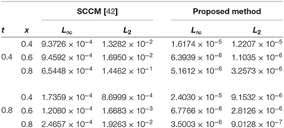
Table 2. Absolute and relative errors for Example 5.1 with M = 100, Δt = 0.001, and α = 1.6.

TABLE 3

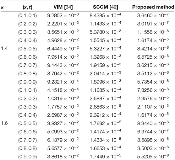
Table 3. Comparison of absolute errors for Example 5.1 using three different methods with M = 100, Δt = 0.001, and α = 1.4 or 1.6.

FIGURE 1

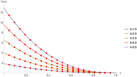
Figure 1. Numerical solution of Example 5.1 with Δt = 0.001, M = 100, and α = 1.5 at different time stages.

FIGURE 2

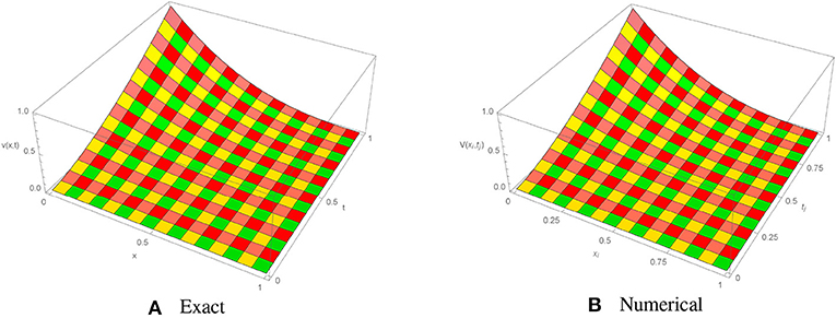
Figure 2. Exact and approximate solutions of Example 5.1 with M = 100, Δt = 0.001, and α = 1.50. (A) Exact. (B) Numerical.

FIGURE 3

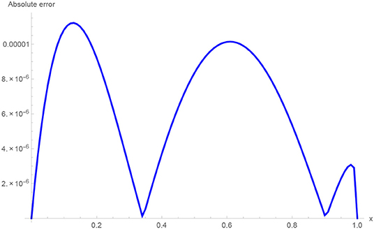
Figure 3. Absolute error for Example 5.1 when M = 100, α = 1.50, and Δt = 0.001.

FIGURE 4

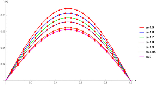
Figure 4. Approximate solution of Example 5.1 with M = 100, t = 0.5, and different values of α.

TABLE 4

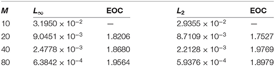
Table 4. Experimental order of convergence (EOC) for Example 5.1 with α = 1.3 and Δt = 0.001.

Example 5.2. Consider the fractional KGE [34, 42]

$\begin{array}{l}\frac{{\partial }^{\alpha }}{\partial t^{\alpha }}v(x,t)-\frac{{\partial }^2}{\partial x^2}v(x,t)+v(x,t)+\frac{3}{2}{v}^3(x,t)=f(x,t),\\ \begin{array}{l}0<x\le 1,0<t\le 1,\end{array}& (41)\end{array}$

where the forcing term f(x, t) on right-hand side is given by

$\begin{array}{l}f(x,t)=\frac{1}{2}\Gamma (3+\alpha )\text{sin}(\pi x)t^2+(1+{\pi }^2)t^{2+\alpha }\text{sin}(\pi x)\\ +\frac{3}{2}[\text{sin}(\pi x)t^{2+\alpha }{]}^3,\end{array}$

For Example 5.2, the piecewise-defined numerical solution obtained using the proposed method with α = 1.5, 0 ≤ x ≤ 1, n = 100, and Δt = 0.01 is given by

$\begin{array}{l}V(x)=\{\begin{array}{cc}8.71156\times 10^{-19}+x(3.13867+x(2.8549\times 10^{-}14+(-4.97167-11.4015x)x))\hfill & \text{if }x\in \left[0.00,0.01\right],\hfill \\ -1.14461\times 10^{-6}+x(3.13904+x(-0.041176+(-3.14329-34.194x)x))\hfill & \text{if }x\in \left[0.01,0.02\right],\hfill \\ -0.0000194466+x(3.14196+x(-0.205754+(0.51013-56.9551x)x))\hfill & \text{if }x\in \left[0.02,0.03\right],\hfill \\ -0.000112001+x(3.15183+x(-0.575584+(5.98188-79.6639x)x))\hfill & \text{if }x\in \left[0.03,0.04\right],\hfill \\ \hfill ⋮\hfill & ⋮\hfill \\ -40.7681+x(339.328+x(-1039.38+(1422.21-733.23x)x))\hfill & \text{if }x\in \left[0.49,0.50\right],\hfill \\ -44.2829+x(360.934+x(-1083.83+(1453.18-733.97x)x))\hfill & \text{if }x\in \left[0.50,0.51\right],\hfill \\ \hfill ⋮\hfill & ⋮\hfill \\ -71.1059+x(298.709+x(-460.613+(312.674-79.6639x)x))\hfill & \text{if }x\in \left[0.96,0.97\right],\hfill \\ -53.5088+x(223.56+x(-340.406+(227.31-56.9551x)x))\hfill & \text{if }x\in \left[0.97,0.98\right],\hfill \\ -34.2394+x(143.149+x(-214.635+(139.919-34.194x)x))\hfill & \text{if }x\in \left[0.98,0.99\right],\hfill \\ -13.2345+x(57.3823+x(-83.3239+(50.5776-11.4015x)x))\hfill & \text{if }x\in \left[0.99,1.00\right].\hfill \end{array}\hfill \end{array}$

The initial/boundary conditions can be extracted from the analytical exact solution v(x, t) = sin(πx)t^2+α. The absolute numerical errors at different grid points of the RECBS solution for Example 5.2 using Δt = 0.001 and M = 100 are listed in Table 5. Again it can be observed that our scheme is more accurate than the SCCM [42]. Table 6 reports the absolute and relative errors in our numerical computation with M = 100, Δt = 0.001, and α = 1.6 at x = 0.4, 0.6, 0.8 when t = 0.4, 0.8. It is clear that the results are better than those obtained by the SCCM [42]. Table 7 compares the absolute errors of the proposed method, VIM [34], and SCCM [42] under different values of α. The EOC in the spatial direction, using Δt = 0.001 and α = 1.50, is tabulated in Table 8. The experimental rate of convergence of the proposed scheme is found to be in line with the theoretical prediction. Figure 5 shows the behavior at different time stages of numerical solutions obtained using α = 1.5, M = 100, and Δt = 0.001. The 3D plots of exact and numerical solutions with α = 1.5 and M = 100 are displayed in Figure 6. The absolute error between the exact and approximate solutions using α = 1.3, M = 100, and Δt = 0.001 is plotted in Figure 7.

TABLE 5

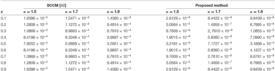
Table 5. Absolute errors for Example 5.2 when M = 100, Δt = 0.001 using different values of α.

TABLE 6

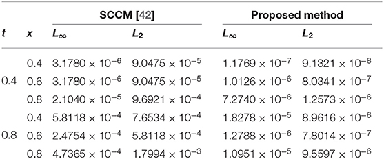
Table 6. Absolute and relative errors for Example 5.2 when M = 100, Δt = 0.001 and α = 1.6.

TABLE 7

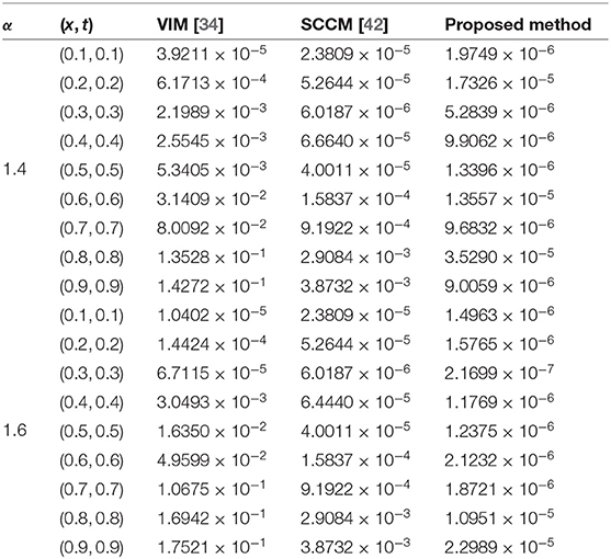
Table 7. Absolute errors for Example 5.2 when M = 100 and Δt = 0.001.

TABLE 8

Table 8. Experimental order of convergence (EOC) for Example 5.2 with α = 1.5 and Δt = 0.001.

FIGURE 5

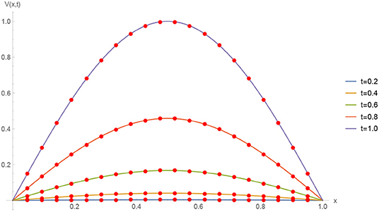
Figure 5. Numerical solution for Example 5.2 with Δt = 0.001, M = 100, and α = 1.5 at different time stages.

FIGURE 6

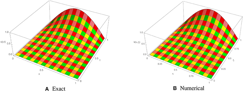
Figure 6. Exact and numerical solutions of Example 5.2 with M = 100, Δt = 0.001, and α = 1.5. (A) Exact. (B) Numerical.

FIGURE 7

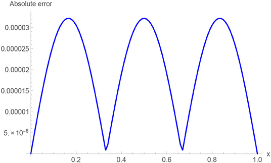
Figure 7. Absolute error for Example 5.2 when M = 100, α = 1.5, and Δt = 0.001.

6. Conclusion

In this work we have conducted a numerical investigation of the time-fractional Klein–Gordon equation by applying the redefined extended cubic B-spline collocation method. A finite central difference formulation is employed for temporal discretization, while a set of redefined extended cubic B-spline functions is used to interpolate the solution curve in the spatial direction. The unconditional stability of the proposed scheme is established, and the orders of convergence along the space and time grids are shown to be O(h²) and O(Δt)^2−α, respectively. The computational outcomes of the proposed algorithm show that the order of convergence agrees with the theoretical results. The numerical scheme has been tested on different problems, and comparison of the results reveals our method's advantage over VIM [34] and SCCM [42].

Author Contributions

All authors listed have made a substantial, direct and intellectual contribution to the work, and approved it for publication.

Conflict of Interest

The authors declare that the research was conducted in the absence of any commercial or financial relationships that could be construed as a potential conflict of interest.

References

1. Rossikhin YA, Shitikova M. Application of fractional derivatives to the analysis of damped vibrations of viscoelastic single mass systems. Acta Mech. (1997) 120:109–25. doi: 10.1007/BF01174319

CrossRef Full Text | Google Scholar

2. Rudolf H. Applications of FractionalCalculus in Physics. Singapore; River Edge, NJ: World Scientific (2000).

Google Scholar

3. Metzler R, Klafter J. The restaurant at the end of the random walk: recent developments in the description of anomalous transport by fractional dynamics. J Phys A Math Gen. (2004) 37:R161. doi: 10.1088/0305-4470/37/31/R01

CrossRef Full Text | Google Scholar

4. Luo MJ, Milovanovic GV, Agarwal P. Some results on the extended beta and extended hypergeometric functions. Appl Math Comput. (2014) 248:631–51. doi: 10.1016/j.amc.2014.09.110

PubMed Abstract | CrossRef Full Text | Google Scholar

5. Zhang Y. Time-fractional Klein-Gordon equation: formulation and solution using variational methods. WSEAS Trans Math. (2016) 15:206–14.

Google Scholar

6. Ruzhansky M, Cho YJ, Agarwal P, Area I. Advances in Real and Complex Analysis With Applications. Singapore: Springer (2017).

Google Scholar

7. Owolabi KM, Hammouch Z. Mathematical modeling and analysis of two-variable system with noninteger-order derivative. Chaos. (2019) 29:013145. doi: 10.1063/1.5086909

PubMed Abstract | CrossRef Full Text | Google Scholar

8. Agarwal P, Baleanu D, Chen Y, Momani S, Machado JAT. Fractional calculus. In: ICFDA: International Workshop on Advanced Theory and Applications of Fractional Calculus. Amman (2019). doi: 10.1007/978-981-15-0430-3

PubMed Abstract | CrossRef Full Text | Google Scholar

9. Babaei A, Jafari H, Ahmadi M. A fractional order HIV/AIDS model based on the effect of screening of unaware infectives. Math Methods Appl Sci. (2019) 42:2334–43. doi: 10.1002/mma.5511

CrossRef Full Text | Google Scholar

10. Babaei A, Jafari H, Liya A. Mathematical models of HIV/AIDS and drug addiction in prisons. Eur Phys J Plus. (2020) 135:395. doi: 10.1140/epjp/s13360-020-00400-0

CrossRef Full Text | Google Scholar

11. Yuste SB, Acedo L. An explicit finite difference method and a new von Neumann-type stability analysis for fractional diffusion equations. SIAM J Numer Anal. (2005) 42:1862–74. doi: 10.1137/030602666

CrossRef Full Text | Google Scholar

12. Sweilam N, Nagy A. Numerical solution of fractional wave equation using Crank-Nicholson method. World Appl Sci J. (2011) 13:71–5.

Google Scholar

13. Ur-Rehman M, Khan RA. The Legendre wavelet method for solving fractional differential equations. Commun Nonlin Sci Numer Simul. (2011) 16:4163–73. doi: 10.1016/j.cnsns.2011.01.014

CrossRef Full Text | Google Scholar

14. Bhrawy A, Tharwat M, Yildirim A. A new formula for fractional integrals of Chebyshev polynomials: application for solving multi-term fractional differential equations. Appl Math Modell. (2013) 37:4245–52. doi: 10.1016/j.apm.2012.08.022

CrossRef Full Text | Google Scholar

15. Rad J, Kazem S, Shaban M, Parand K, Yildirim A. Numerical solution of fractional differential equations with a Tau method based on Legendre and Bernstein polynomials. Math Methods Appl Sci. (2014) 37:329–42. doi: 10.1002/mma.2794

CrossRef Full Text | Google Scholar

16. Mohebbi A, Abbaszadeh M, Dehghan M. High-order difference scheme for the solution of linear time fractional Klein-Gordon equations. Numer Methods Partial Differ Equat. (2014) 30:1234–53. doi: 10.1002/num.21867

CrossRef Full Text | Google Scholar

17. Heydari M, Hooshmandasl M, Mohammadi F, Cattani C. Wavelets method for solving systems of nonlinear singular fractional Volterra integro-differential equations. Commun Nonlin Sci Numer Simul. (2014) 19:37–48. doi: 10.1016/j.cnsns.2013.04.026

CrossRef Full Text | Google Scholar

18. Salahshour S, Ahmadian A, Senu N, Baleanu D, Agarwal P. On analytical solutions of the fractional differential equation with uncertainty: application to the basset problem. Entropy. (2015) 17:885–902. doi: 10.3390/e17020885

CrossRef Full Text | Google Scholar

19. Sweilam N, Nagy A, El-Sayed AA. Second kind shifted Chebyshev polynomials for solving space fractional order diffusion equation. Chaos Solit Fract. (2015) 73:141–7. doi: 10.1016/j.chaos.2015.01.010

CrossRef Full Text | Google Scholar

20. Ramezani M, Jafari H, Johnston SJ, Baleanu D. Complex b-spline collocation method for solving weakly singular Volterra integral equations of the second kind. Miskolc Math Notes. (2015) 16:1091–103. doi: 10.18514/MMN.2015.1469

CrossRef Full Text | Google Scholar

21. Badr M, Yazdani A, Jafari H. Stability of a finite volume element method for the time-fractional advection-diffusion equation. Numer Methods Partial Differ Equat. Wiley online Library. (2018) 34:1459–71. doi: 10.1002/num.22243

CrossRef Full Text | Google Scholar

22. Agarwal P, Agarwal RP, Ruzhansky M. Special Functions and Analysis of Differential Equations. (2020).

Google Scholar

23. Atangana A, Secer A. A note on fractional order derivatives and table of fractional derivatives of some special functions. Abstr Appl Anal. (2013) 2013:279681. doi: 10.1155/2013/279681

CrossRef Full Text | Google Scholar

24. Srivastava H, Agarwal P. Certain fractional integral operators and the generalized incomplete hypergeometric functions. Appl Appl Math. (2013) 8:333–45.

Google Scholar

25. Goufo EFD. Solvability of chaotic fractional systems with 3D four-scroll attractors. Chaos Solit Fract. (2017) 104:443–51. doi: 10.1016/j.chaos.2017.08.038

CrossRef Full Text | Google Scholar

26. Asif N, Hammouch Z, Riaz M, Bulut H. Analytical solution of a Maxwell fluid with slip effects in view of the Caputo-Fabrizio derivative. Eur Phys J Plus. (2018) 133:272. doi: 10.1140/epjp/i2018-12098-6

CrossRef Full Text | Google Scholar

27. Singh J, Kumar D, Hammouch Z, Atangana A. A fractional epidemiological model for computer viruses pertaining to a new fractional derivative. Appl Math Comput. (2018) 316:504–15. doi: 10.1016/j.amc.2017.08.048

CrossRef Full Text | Google Scholar

28. Atangana A, Goufo EFD. Conservatory of Kaup-Kupershmidt equation to the concept of fractional derivative with and without singular kernel. Acta Math Appl Sin. (2018) 34:351–61. doi: 10.1007/s10255-018-0757-7

CrossRef Full Text | Google Scholar

29. Owolabi KM, Atangana A. Computational study of multi-species fractional reaction-diffusion system with ABC operator. Chaos Solit Fract. (2019) 128:280–9. doi: 10.1016/j.chaos.2019.07.050

CrossRef Full Text | Google Scholar

30. Uçar S, Uçar E, Özdemir N, Hammouch Z. Mathematical analysis and numerical simulation for a smoking model with Atangana-Baleanu derivative. Chaos Solit Fract. (2019) 118:300–6. doi: 10.1016/j.chaos.2018.12.003

CrossRef Full Text | Google Scholar

31. Goufo EFD, Toudjeu IT. Analysis of recent fractional evolution equations and applications. Chaos Solit Fract. (2019) 126:337–50. doi: 10.1016/j.chaos.2019.07.016

CrossRef Full Text | Google Scholar

32. Batiha B, Noorani MSM, Hashim I. Numerical solution of sine-Gordon equation by variational iteration method. Phys Lett A. (2007) 370:437–40. doi: 10.1016/j.physleta.2007.05.087

CrossRef Full Text | Google Scholar

33. Yusufoğlu E. The variational iteration method for studying the Klein-Gordon equation. Appl Math Lett. (2008) 21:669–74. doi: 10.1016/j.aml.2007.07.023

CrossRef Full Text | Google Scholar

34. Odibat Z, Momani S. The variational iteration method: an efficient scheme for handling fractional partial differential equations in fluid mechanics. Comput Math Appl. (2009) 58:2199–208. doi: 10.1016/j.camwa.2009.03.009

CrossRef Full Text | Google Scholar

35. Jafari H, Saeidy M, Arab Firoozjaee M. Solving nonlinear Klein-Gordon equation with a quadratic nonlinear term using homotopy analysis method. Iran J Optimiz. (2010) 2:130–38.

Google Scholar

36. Jafari H, Khalique CM, Ramezani M, Tajadodi H. Numerical solution of fractional differential equations by using fractional B-spline. Central Eur J Phys. (2013) 11:1372–6. doi: 10.2478/s11534-013-0222-4

CrossRef Full Text | Google Scholar

37. Vong S, Wang Z. A compact difference scheme for a two dimensional fractional Klein-Gordon equation with Neumann boundary conditions. J Comput Phys. (2014) 274:268–82. doi: 10.1016/j.jcp.2014.06.022

CrossRef Full Text | Google Scholar

38. Vong S, Wang Z. A high-order compact scheme for the nonlinear fractional Klein-Gordon equation. Numer Methods Partial Differ Equat. (2015) 31:706–22. doi: 10.1002/num.21912

CrossRef Full Text | Google Scholar

39. Dehghan M, Abbaszadeh M, Mohebbi A. An implicit RBF meshless approach for solving the time fractional nonlinear sine-Gordon and Klein-Gordon equations. Eng Anal Bound Elements. (2015) 50:412–34. doi: 10.1016/j.enganabound.2014.09.008

CrossRef Full Text | Google Scholar

40. Jafari H. Numerical solution of time-fractional Klein-Gordon equation by using the decomposition methods. J Comput Nonlin Dyn. (2016) 11:041015. doi: 10.1115/1.4032767

CrossRef Full Text | Google Scholar

41. Chen H, Lü S, Chen W, et al. A fully discrete spectral method for the nonlinear time fractional Klein-Gordon equation. Taiwan J Math. (2017) 21:231–51. doi: 10.11650/tjm.21.2017.7357

CrossRef Full Text | Google Scholar

42. Nagy A. Numerical solution of time fractional nonlinear Klein-Gordon equation using Sinc-Chebyshev collocation method. Appl Math Comput. (2017) 310:139–48. doi: 10.1016/j.amc.2017.04.021

CrossRef Full Text | Google Scholar

43. Kanwal A, Phang C, Iqbal U. Numerical solution of fractional diffusion wave equation and fractional Klein-Gordon equation via two-dimensional Genocchi polynomials with a Ritz-Galerkin method. Computation. (2018) 6:40. doi: 10.3390/computation6030040

CrossRef Full Text | Google Scholar

44. Lyu P, Vong S. A linearized second-order scheme for nonlinear time fractional Klein-Gordon type equations. Numer Algorithms. (2018) 78:485–511. doi: 10.1007/s11075-017-0385-y

CrossRef Full Text | Google Scholar

45. Doha E, Abdelkawy M, Amin A, Lopes AM. A space-time spectral approximation for solving nonlinear variable-order fractional sine and Klein-Gordon differential equations. Comput Appl Math. (2018) 37:6212–29. doi: 10.1007/s40314-018-0695-2

CrossRef Full Text | Google Scholar

46. Amin M, Abbas M, Iqbal MK, Ismail AIM, Baleanu D. A fourth order non-polynomial quintic spline collocation technique for solving time fractional superdiffusion equations. Adv Differ Equat. (2019) 2019:1–21. doi: 10.1186/s13662-019-2442-4

CrossRef Full Text | Google Scholar

47. Khalid N, Abbas M, Iqbal MK, Baleanu D. A numerical algorithm based on modified extended B-spline functions for solving time-fractional diffusion wave equation involving reaction and damping terms. Adv Differ Equat. (2019) 2019:378. doi: 10.1186/s13662-019-2318-7

CrossRef Full Text | Google Scholar

48. Wasim I, Abbas M, Iqbal M. A new extended B-spline approximation technique for second order singular boundary value problems arising in physiology. J Math Comput Sci. (2019) 19:258–67. doi: 10.22436/jmcs.019.04.06

CrossRef Full Text | Google Scholar

49. Sharifi S, Rashidinia J. Numerical solution of hyperbolic telegraph equation by cubic B-spline collocation method. Appl Math Comput. (2016) 281:28–38. doi: 10.1016/j.amc.2016.01.049

CrossRef Full Text | Google Scholar

50. Khalid N, Abbas M, Iqbal MK, Baleanu D. A numerical investigation of Caputo time fractional Allen-Cahn equation using redefined cubic B-spline functions. Adv Differ Equat. (2020) 2020:1–22. doi: 10.1186/s13662-020-02616-x

CrossRef Full Text | Google Scholar

51. De Boor C. On the convergence of odd-degree spline interpolation. J Approx Theory. (1968) 1:452–63. doi: 10.1016/0021-9045(68)90033-6

CrossRef Full Text | Google Scholar

52. Hall CA. On error bounds for spline interpolation. J Approx Theory. (1968) 1:209–18. doi: 10.1016/0021-9045(68)90025-7

CrossRef Full Text | Google Scholar

53. Iqbal MK, Abbas M, Zafar B. New quartic B-spline approximations for numerical solution of fourth order singular boundary value problems. Punjab Univ J Math. (2020) 52:47–63.

Google Scholar

54. Wasim I, Abbas M, Amin M. Hybrid B-spline collocation method for solving the generalized Burgers-Fisher and Burgers-Huxley equations. Math Probl Eng. (2018) 2018:6143934. doi: 10.1155/2018/6143934

CrossRef Full Text | Google Scholar