 Xue Zhang
 Juntao Wang
- 1China Institute of Rural Education Development, Northeast Normal University, Changchun, China
- 2School of Mathematics and Statistics, Northeast Normal University, Changchun, China
Model data fit plays an important role in any statistical analysis, and the primary goal is to detect the preferred model based on certain criteria. Under the cognitive diagnostic assessment (CDA) framework, a family of sequential cognitive diagnostic models (CDMs) is introduced to handle polytomously scored data, which are attained by answering constructed-response items sequentially. The presence of attribute hierarchies, which can provide useful information about the nature of attributes, will help understand the relation between attributes and response categories. This article introduces the sequential hierarchical CDM (SH-CDM), which adapts the sequential CDM to deal with attribute hierarchy. Furthermore, model fit analysis for SH-CDMs is assessed using eight model fit indices (i.e., three absolute fit indices and five relative fit indices). Two misfit sources were focused; that is, misspecifying attribute structures and misfitting processing functions. The performances of those indices were evaluated via Monte Carlo simulation studies and a real data illustration.
Introduction
Cognitive diagnostic assessment (CDA) has gained widespread use since its introduction, as it can provide fine-grained feedback through pinpointing the presence or absence of multiple fine-grained skills or attributes (Leighton and Gierl, 2007; Templin and Bradshaw, 2013) based on some cognitive diagnostic models (CDMs). Many different names according to their different connotations (Rupp et al., 2010; Ma, 2017) can be applied to refer to the CDM, in which the diagnostic classification model (DCM; Rupp et al., 2010) is most widely applied.
For dichotomously scored items, a number of CDMs can be found in literature, among others, the deterministic inputs, noisy “and” gate (DINA; Haertel, 1989; Junker and Sijtsma, 2001) model, the deterministic inputs, noisy “or” gate (DINO; Templin and Henson, 2006) model, and the additive CDM (A-CDM; de la Torre, 2011) were most widely used. Furthermore, three most general CDMs, the general diagnostic model (GDM; von Davier, 2008), the log-linear CDM (LCDM; Henson et al., 2009), and the generalized deterministic input noisy and gate model (GDINA; de la Torre, 2011), were proposed to better understand and handle the above models. Specifically, the GDINA model is equivalent to the LCDM when the logit link is used, and the GDM is a general version of both of them.
For polytomously scored items, which yield graded responses with ordered categories or nominal responses, a few models have been developed, such as the GDM for graded response (von Davier, 2008), the nominal response diagnostic model (NRDM; Templin et al., 2008), the partial credit DINA model (de la Torre, 2010), the polytomous LCDM (Hansen, 2013), the sequential CDM (sCDM; Ma and de la Torre, 2016), and the diagnostic tree model (DTM; Ma, 2019). Among them, only sCDM and DTM can model the possible relation between attributes and response categories. Furthermore, Liu and Jiang (2020) proposed the rating scale diagnostic model (RSDM), which was a special version of the NRDM with fewer parameters. Culpepper (2019) presented an exploratory diagnostic framework for ordinal data.
On the other hand, attribute dependencies often occur in practical applications, instead of that all attributes are independent for each examinee. To this end, four different types of attribute hierarchies (i.e., linear, convergent, divergent, and unstructured) were considered to reflect attribute dependencies (Gierl et al., 2007). An example of different types of attribute hierarchies is shown in Figure 1. For an external shape, a directed acyclic graph (DAG) is used to express the attribute hierarchy; and for an internal organization, all possible attribute profiles are provided. Let α1, α2, α3, α4 denote four attributes measured by a CDA. Take the linear structure as an example, αk is the prerequisite of αk+1 (k = 1, 2, 3), as a result, the number of all possible attribute patterns is 5, which is less than 24 = 16. To model attribute hierarchy, Templin and Bradshaw (2014) proposed a hierarchical diagnostic classification model (HDCM). Zhan et al. (2020) proposed a sequential higher-order DINA model with attribute hierarchy to handle the higher-order and hierarchical structures simultaneously using the sequential tree. Interested readers can refer to Rupp et al. (2010) and von Davier and Lee (2019) for detailed information.
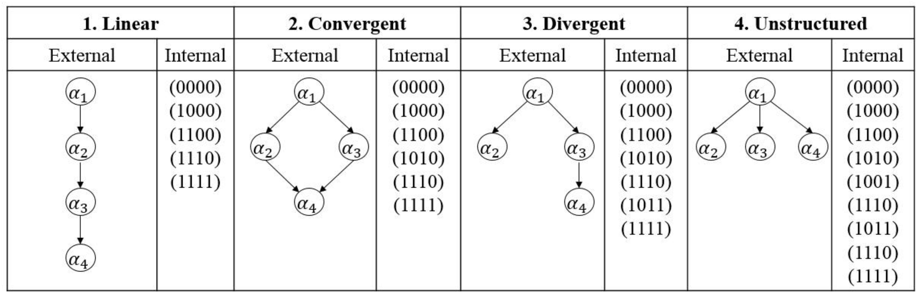
Figure 1. Types of hierarchical attribute structures. For the convergent structure, mastering α4 needs to master both α2 and α3 (Zhan et al., 2020), as well as α1.
It is a central concern to assess global-level fit (i.e., model fit) in the psychometric area. Model fit analysis can be evaluated by two aspects: absolute fit analysis, which assesses how well a given model reproduces the sample data directly; and relative fit analysis, which recommends a better-fit model through comparing at least two candidates. Under the CDA framework, the sources of model misfit include inaccurate item response function (IRF), Q-matrix misspecification, misspecifying attribute pattern structures (Han and Johnson, 2019), abnormal response behaviors (e.g., rapid guessing, and cheating), local item dependence, and so on.
Regarding absolute fit assessment, for the sequential GDINA model, Ma and de la Torre (2019) proposed category-level model selection criteria based on the Wald test and the likelihood ratio (LR) test to identify different IRFs; and Ma (2020) used limited-information indices [i.e., Mord and standardized mean square root of squared residual (SRMSR)] to detect model misspecification or Q-matrix misspecification. On the other hand, Lim and Drasgow (2019) proposed the Mantel–Haenszel (MH) chi-square statistic to detect latent attribute misspecification in non-parametric cognitive diagnostic methods.
In terms of relative fit assessment, Sen and Bradshaw (2017) compared the Akaike information criterion (AIC), Bayesian information criterion (BIC), and adjusted BIC (aBIC), and found that they performed poorly to differentiate CDMs and multidimensional item response theory (MIRT) models for dichotomous response data.
Furthermore, some researches focused on the performances of both absolute fit indices (AFIs) and relative fit indices (RFIs) for dichotomous CDMs. Under Bayesian framework, Sinharay and Almond (2007) used Bayesian residuals, which are based on the individuals’ raw scores, as AFI and deviance information criterion (DIC) as RFI to distinguish different measurement models. Chen et al. (2013) used both AFIs [i.e., abs(fcor), residuals based on the proportion correct of individual items and the log-odds ratios of item pairs] and RFIs (i.e., -2LL, AIC, and BIC) to identify model and/or Q-matrix misspecifications. Hu et al. (2016) investigated the usefulness of AIC, BIC, and consistent AIC (CAIC) as RFIs, and limited information root mean square error of approximation (RMSEA2), abs(fcor), and max() as AFIs to detect model or Q-matrix misspecification. Lei and Li (2016) detected model and Q-matrix misspecifications using AFIs [i.e., RMSEA, mean of absolute values of Q3 statistic (MADQ3), mean of absolute values of pairwise item covariance residuals (MADres), mean of absolute deviations in observed and expected correlations (MADcor), and mean of all item pair statistics (M)] and RFIs (i.e., AIC and BIC). Empirically, Han and Johnson (2019) assessed global-level fit for dichotomous CDMs using both RFIs (i.e., AIC, BIC, and aBIC) and AFIs [i.e., M2, RMSEA2, and maximum of all item pair statistics (max())] through a real data illustration.
As no prior studies have analyzed the CDM fit for polytomous response data with attribute hierarchy, the current study concentrates on a novel model, named as the sequential hierarchical CDM (SH-CDM), and assesses model-data fit. This study provides important evidence and insight to support the usefulness of SH-CDMs in the future. The remainder of this article is listed as follows. First, we introduce the sequential hierarchical CDMs and review different model fit indices. Next, simulation studies and a real data illustration are provided to evaluate the performances of those indices. Finally, we end with some concluding remarks. Supplementary Appendix A and Supplementary Material are provided to complement the detailed information and simulation results.
Materials and Methods
Model Description
In this section, SH-CDMs are introduced based on Templin and Bradshaw (2014) and Ma and de la Torre (2016). The sCDM (Ma and de la Torre, 2016) is a special version of SH-CDM with non-hierarchical attribute structure, and the HDCM (Templin and Bradshaw, 2014) is a special version of SH-CDM when all response data are scored dichotomously.
To analyze the polytomously scored data from constructed-response items, the sCDM is built upon a sequential process model. As a result, it can provide the detailed problem-solving procedures to support subsequent inference. For a constructed-response test with J items, assuming item j (j = 1, 2, …, J) involves Hj tasks that need to be solved sequentially; therefore, if the 1st task is failed, the score should be 0; if the first h (0 < h < Hj) tasks are successful but the (h + 1)th task is failed, the score should be h; else if all tasks are successful, the score should be Hj. To this end, Ma and de la Torre (2016) proposed a –by–K category-level matrix, named as the Qc-matrix, the element of which is a binary indicator of whether the task of the corresponding item measures this attribute. In this article, only the restricted Qc-matrix is considered. Mathematically, let Qc = {qjh,k}, qjh,k = 1 if attribute k (k = 1, 2, … K) is measured by item j for task h (h = 1, 2, …, Hj), otherwise, qjh,k = 0.
Let the processing function, Sjh, be the probability of examinees with attribute pattern answering the firsth tasks of item j correctly given answering the first (h-1)th tasks correctly, where g = 1, 2, …, G, and G denotes the total number of latent classes. Notating as the reduced attribute profile of examinee l (l = 1, 2, …, N), which contains all the required attributes of item j for task h. Then, . In this article, the DINA model, DINO model, A-CDM, and GDINA model are considered, which represent the conjunctive, disjunctive, additive, and general condensation rules, respectively. Hereafter, only the identity link is considered for the GDINA model, which is equivalent to the logit link1. Assuming that all categories share the same condensation rule, let be the total number of required attributes by item j for task h; the expressions for processing functions are summarized in Table 1.
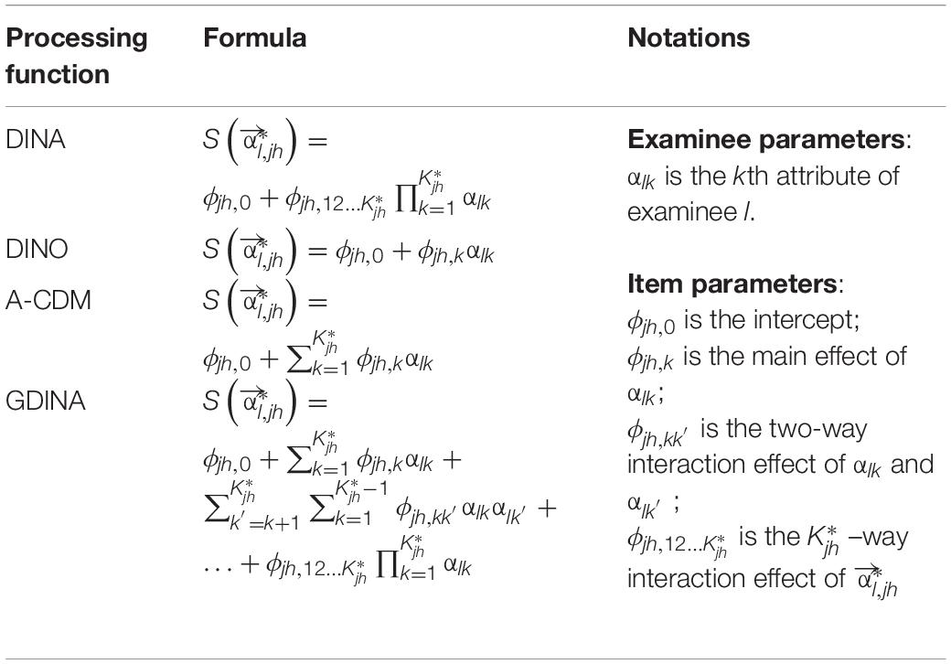
Table 1. Summary of S() for different processing functions.
Furthermore, the existence of attribute hierarchy will reduce the model complexity of IRF. To deal with attribute hierarchies, the HDCM was proposed by Templin and Bradshaw (2014). As the HDCM is nested within more general CDMs, the SH-CDM is introduced by combining it with the sCDM. In the SH-CDM, the influence of attribute hierarchy is reflected in the processing function. Take the SH-GDINA model as an example, assuming four linear attributes (Figure 1) are measured in the test and three attributes are required by item j for task h, , where the subscript of k denotes the order of the required attributes.
To ensure joint identifiability of the HDCMs, Gu and Xu (2019) restricted that the sparsified version of Q-matrix had at least three entries of “1”s in each column and Q-matrix can be rearranged as , where Q0 was equivalent to a K-by-K identity matrix IK under the attribute hierarchy and the densified version of Q∗ contained K distinct column vectors. In addition, if Q-matrix was constrained to contain an IK, the HDCMs were identified. The SH-CDM identifiability shares the same restrictions as those mentioned above. Interested reader can refer to Gu and Xu (2019) for further discussion on model identifiability.
Model Fit Indices
To assess global-level fit of CDMs, both absolute fit assessment and relative fit assessment are done to identify adequate-fit models and select the best-fit model, respectively. To ensure the comparability of different AFIs, SRMSR, 100∗MADRESIDCOV, and MADcor are considered as they share the same rule. To choose the best-fit model among all candidates, five widely used RFIs [i.e., AIC, BIC, the second-order information criterion (AICc), aBIC, and CAIC] are evaluated and compared.
Absolute Fit Index
The SRMSR (Maydeu-Olivares, 2013) is a measure of pairwise correlations. As a standardized statistic, test length has few influences on the performance of SRMSR. The SRMSR can be calculated as
where rjj’ and denote the observed and predicted pairwise item correlations, respectively. The model with smaller SRMSR will be identified as a good fit one.
The mean absolute deviation (MAD) is a fundamental statistic to calculate the last two AFIs mentioned before, which measures the discrepancy between the observed item conditional probabilities of success and the predicted ones. The RESIDCOV denotes the residual covariance of pairwise items. Then, we can obtain the mean of absolute deviations of residual covariances (MADRESIDCOV; McDonald and Mok, 1995) by replacing the conditional probabilities in MAD by the RESIDCOVs. The MADRESIDCOV measures the discrepancy between observed and predicted pairwise item residual covariance (RESIDCOV). Let,
Then, we can obtain
100∗MADRESIDCOV is used equivalently, as the magnitude of MADRESIDCOV is usually small. The MADcor (DiBello et al., 2007) is the mean of absolute deviations in observed and expected correlations of pairwise items. The MADcor equals, where rjj’ and have the same meanings as those in SRMSR. For MAD-type indices, a smaller value (i.e., value near to zero) denotes better fit.
Relative Fix Index
Different types of information criteria are calculated with respect to the penalty term, the expressions of which are presented in Table 2. AIC (Akaike, 1974) and BIC (Schwarz, 1978) are most widely applied since their introductions. The second-order information criterion (AICc; Sugiura, 1978) was derived to deal with the small ratio of sample size to estimated number of parameters case (i.e., less than 40; Burnham and Anderson, 2002). As the sample size gets large, AICc converges to AIC. The aBIC (Sclove, 1987) modified BIC by adjusting the sample size term to handle the small sample size case well. The CAIC was proposed by Bozdogan (1987), in which then penalty terms include both the order of the model and the sample size. The candidate model with smaller RFI is recommended.
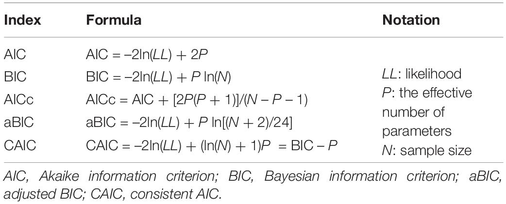
Table 2. Formulas of different relative fit indices.
Simulation Studies
The simulation studies aim (a) to examine parameter recovery for SH-CDMs and (b) to compare the performances of different AFIs and RFIs for SH-CDMs. Two different sources of misfit are considered: the first type of misfit is due to attribute structures misspecification, and the second type of misfit relies on different processing functions. To this end, three simulation studies are conducted: (I) to examine whether parameters of SH-CDMs can be recovered well; (II) to investigate the performances of model fit indices to identity attribute structures; and (III) to investigate their performances to detect the processing function misspecification, respectively.
The simulation conditions are summarized in Table 3. More details will be given in the simulation design sections. In this article, the GDINA R package (Ma and de la Torre, 2020) was used to estimate different SH-CDMs and assess the model fit. The source code including the computation of indices, which were not provided in the GDINA R package, was provided in Supplementary Appendix A. The mapping matrix method (Tutz, 1997) and the expected a posteriori (EAP) method, which are the default methods in the GDINA package for sequential CDMs, were used to estimate item parameters and attribute profiles, respectively. Five hundred replications were conducted for each condition.
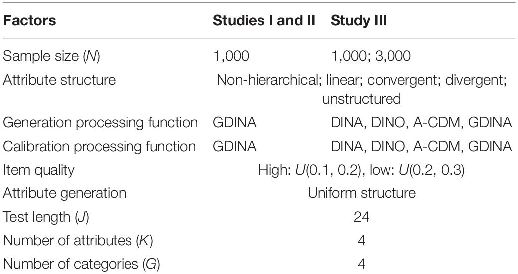
Table 3. Summary of simulation conditions.
Study Design I
In this study, the GDINA model was chosen as the processing function, as its generality. Attribute profiles were generated from the uniform structure; that is, all the possible latent classes shared the same probability. Sample size was 1,000. A 24-item test, in which there were 20 four-category items and four dichotomously scored items, was used. For four-category items, four attributes were measured totally and no more than three attributes were required by each item. Without loss of generality, the last four items were dichotomously scored with an identity subQ-matrix to ensure model identifiability. Two manipulated factors included attribute structure (non-hierarchical, linear, convergent, divergent, and unstructured) and item quality (high and low). For each data set, item parameters and attribute profiles were simulated separately and the Q-matrix was kept consistent.
The item parameter recovery was calculated in terms of average root mean square error (RMSE), average bias, and average relative absolute bias (RAbias), and the classification accuracies were examined using pattern-wise agreement rate (PAR) and attribute-wise agreement rate (AAR).
Simulation Result I
Hereafter, for convenience, let S1 = the SH-GDINA model with non-hierarchical attribute structure; S2 = the SH-GDINA model with linear attribute structure; S3 = the SH-GDINA model with convergent attribute structure; S4 = the SH-GDINA model with divergent attribute structure; S5 = the SH-GDINA model with unstructured attribute structure.
Table 4 summarizes the estimation accuracy and precision of SH-GDINA models. For different attribute structures, attribute profiles in high item quality cases could be recovered better than in the corresponding low item quality cases. The estimation accuracy of item parameters had a similar trend except for convergent attribute structure cases, although the values of RMSE and bias in low item quality cases were smaller than those in high item quality cases, which is because true item parameters’ values in the low cases were smaller, and the smaller true values led to larger RAbiases.
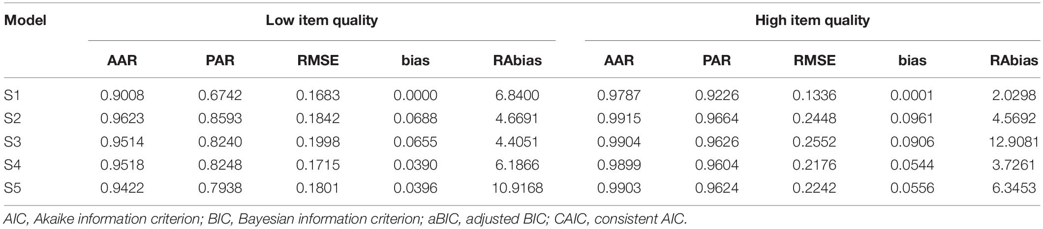
Table 4. Summary of parameter recovery when CM = GM.
Furthermore, the SH-GDINA model with non-hierarchical attribute structure, which was the most general one among these models, was used to fit response data generated by different SH-GDINA models. The parameter recovery is summarized in Table 5. Compared with results shown in Table 4, AAR and PAR were smaller, and RMSE and RAbias were larger. It appears that specifying the attribute hierarchy can significantly improve the estimation accuracy and precision, which supports the introduction of SH-CDMs.
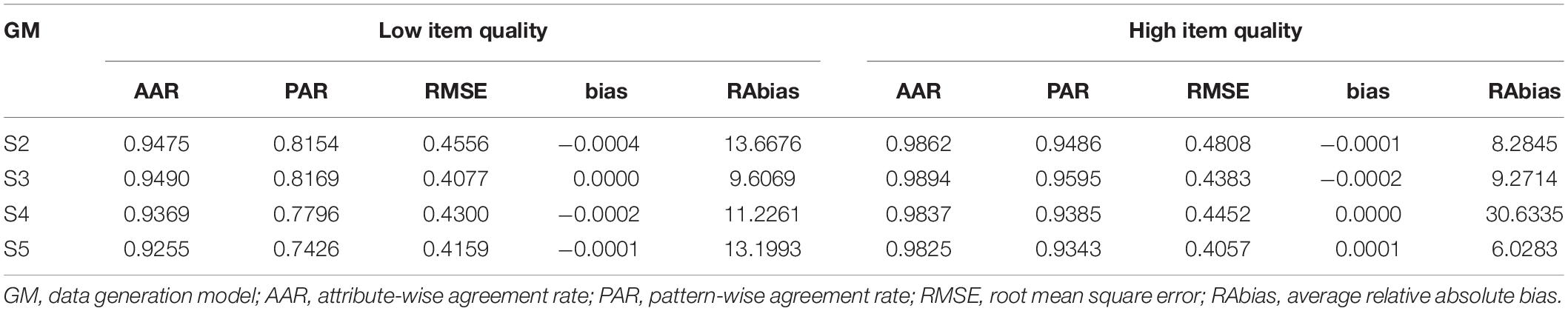
Table 5. Summary of parameter recovery when data were fitted by S1.
Study Design II
In this study, the same simulation settings as the simulation study I were considered. Correct detection rates (CDRs) were used to evaluate the performances of different indices. For AFIs, as there is no sufficient evidence for the cutoff values of these AFIs to support model fit assessment, the CDR is calculated as the rate of the smallest values for all replications. Meanwhile, the box plot of AFIs is also provided to compare the performances of different AFIs intuitively.
Simulation Result II
A popular rule for AIC (Burnham and Anderson, 2002) is that a difference of 2 or less is considered negligible and a difference exceeding 10 constitutes strong support. In this article, the same rule is used for all the RFIs. For the non-hierarchical attribute structure, all AFIs of the data generation model had the smallest values, and all RFIs recommended the true model with strong support. For hierarchical attribute structures, Tables 6, 7 provide CDRs of RFIs and AFIs, respectively.
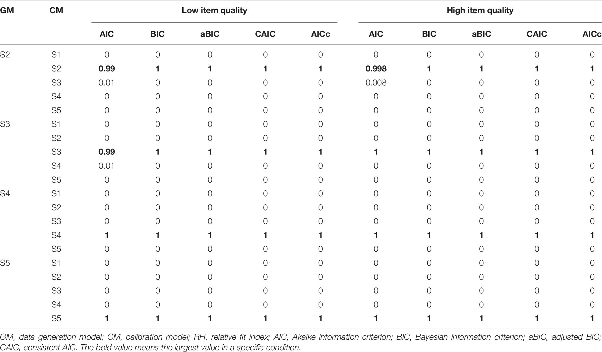
Table 6. Correct detection rates of RFIs for different hierarchical attribute structures.
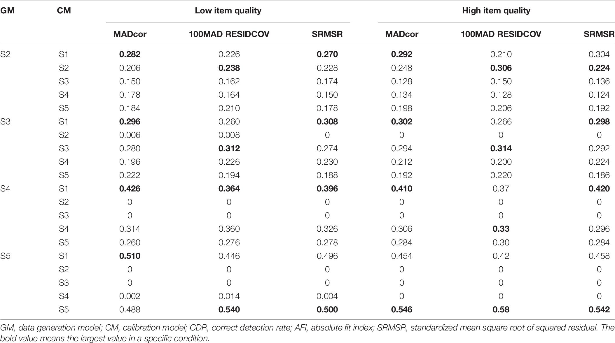
Table 7. CDRs of AFIs for different hierarchical attribute structures.
As shown in Table 6, all RFIs could select the true model with a probability larger than 0.99. Regarding the effectiveness of detecting distinguished models with similar RFIs, we calculated the rates of the differences between RFI values of two candidates, which were smaller than 10, and named as the indistinguishable proportion. When response data were generated by S2, the indistinguishable proportions of AIC to differentiate S3 were 4.8% and 27.2% for the high item quality case and the low item quality case, respectively; and the indistinguishable proportion of AICc was 0.2% for the high item quality case. To generate response data using S3, for the high item quality case, the indistinguishable proportion of AIC to differentiate S4 was 3.8%; for the low item quality case, the indistinguishable proportion of AIC to differentiate S4 was 29%, among them 1% of the time AIC could not differentiate S3, S4, and S5. For the case in which data were generated by S4, the indistinguishable proportion of AIC to differentiate S4 and S5 was less than 6%. Other cases could be differentiated well.
In terms of AFIs (Table 7), S1 mostly had the smallest AFIs. The CDRs of different AFIs were similar. According to the box plots of AFIs (Figures 2, 3), when generating data using S2, it was very hard to differentiate these models. Similarly, it was difficult to distinguish S3 from S1 and S5, S4 from S1 and S5, or S5 from S1. High item quality led to large values of AFIs. It appears that RFIs outperform AFIs for SH-GDINA models, and RFIs distinguish SH-GDINA models with convergent attribute structures from models with unstructured attribute structures with difficulty.
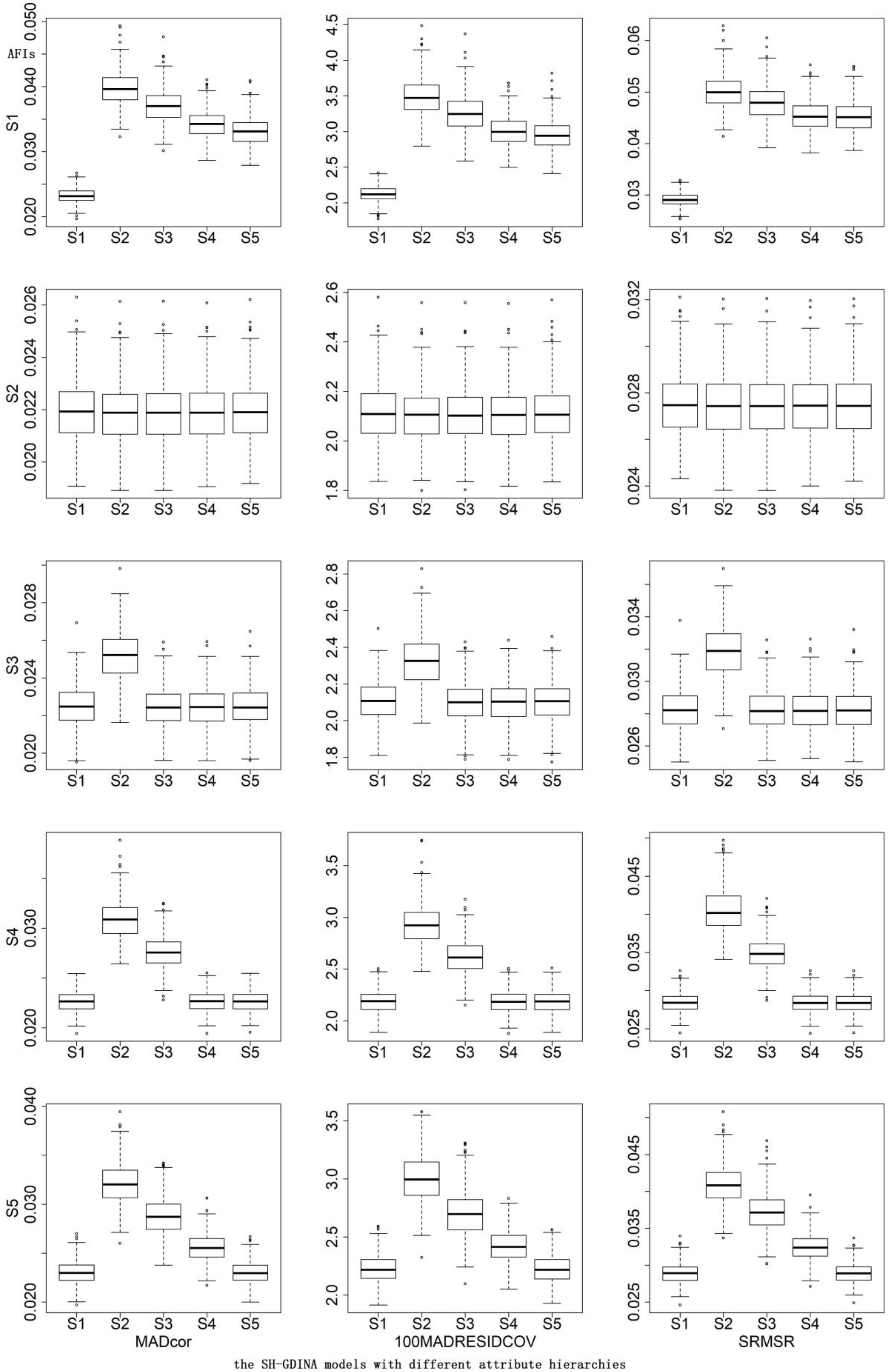
Figure 2. Box plots of absolute fit indices (AFIs) in low item quality cases of simulation study II.
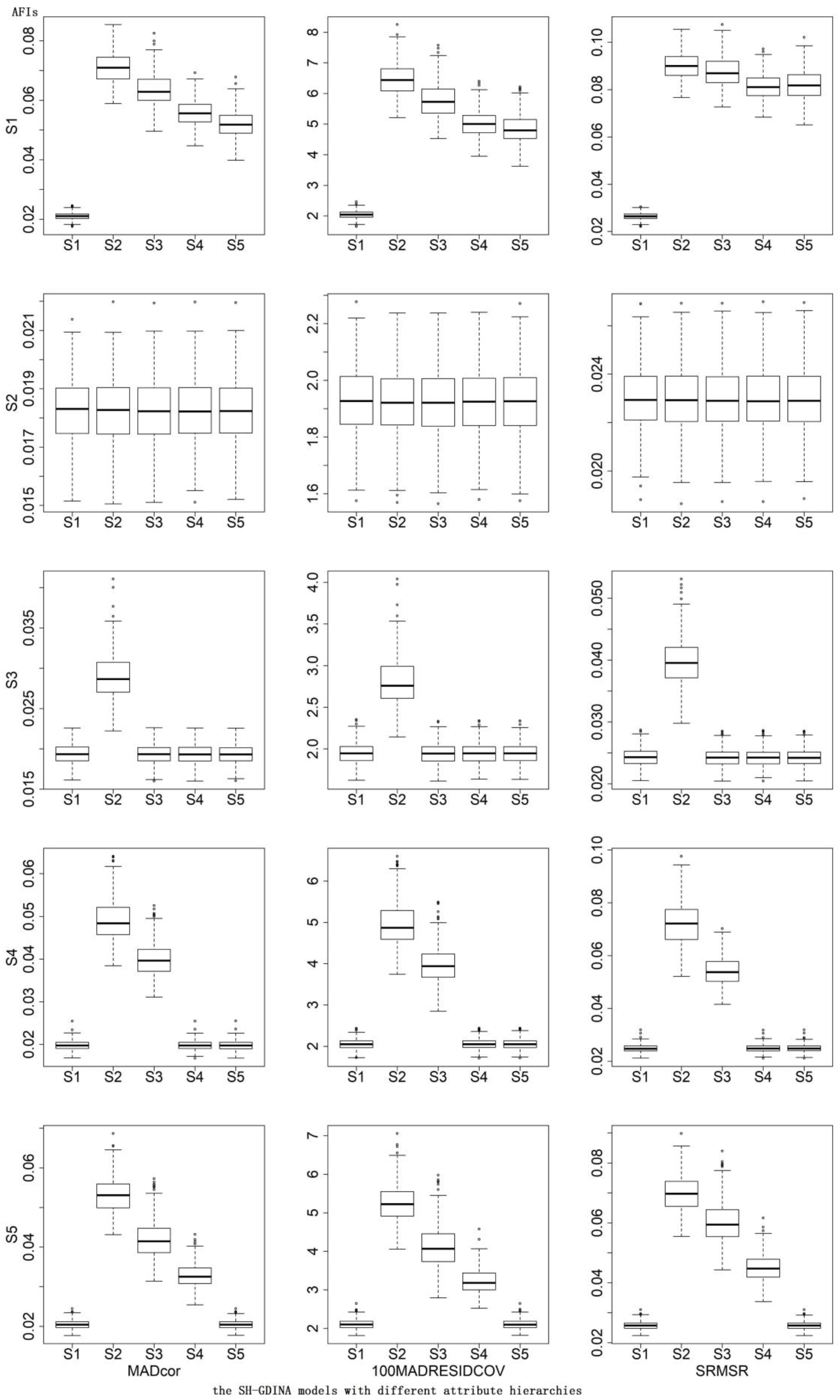
Figure 3. Box plots of absolute fit indices (AFIs) in high item quality cases of simulation study II.
Simulation Design III
In this study, attribute generation method, test length, and test structure were kept the same as those in simulation studies I and II. The manipulated factors included sample size (1,000 and 3,000), attribute structure (non-hierarchical, linear, convergent, divergent, and unstructured), item quality (high and low), and data generation/calibration model (SH-DINA, SH-DINO, SH-ACDM, and SH-GDINA). To evaluate the performances of different indices, the CDRs were reported. Hence, item parameters and the Q-matrix were fixed for each condition, and attribute profiles were simulated separately.
Simulation Result III
For convenience, let M1 = the SH-DINA model, M2 = the SH-DINO model, M3 = the SH-ACDM, and M4 = the SH-GDINA model.
Relative Fit Index
Limited by the space, we only provided the results when the probabilities of true model selection by different RFIs were different or incorrect in Table 8. The whole results (i.e., CDRs of both RFIs and AFIs, box plots of AFIs) were provided in the Supplementary Material. The different performances were reflected in the SH-ACDM and the SH-GDINA model. Under the conditions mentioned in Table 8, AIC and AICc always chose the true model, BIC and CAIC always chose the alternative model, and aBIC mostly selected the true model. Besides, for linear attribute structures, when the data generation model was the SH-ACDM, all RFIs recommended the SH-GDINA model with a probability larger than 0.98. In other cases, all RFIs could select the data generation model as the better fitting one with a probability larger than 0.93.
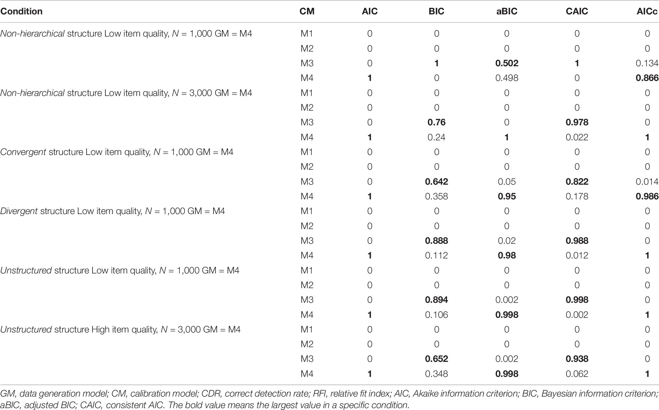
Table 8. Selected results of CDRs of RFIs for different models.
When data were generated by M4 with non-hierarchical attribute structures, in low item quality cases, the indistinguishable proportions of aBIC and AICc to differentiate M3 and M4 were about 10% for a small sample size; for a large sample size, BIC could not differentiate M3 and M4 5.4% of the time and the indistinguishable proportion of CAIC was 1%.
For linear attribute structures, AIC could not distinguish M1 from M3 or M4 for one or two replications under different conditions. When the generation model was M2, the indistinguishable proportions of AIC with high item quality were similar to those in the “GM = M1” case. When response data were generated by M3 or M4, all RFIs could not differentiate M3 and M4.
For convergent attribute structures, AIC could not distinguish M2 from M4 in no more than one replication under different conditions. M3 and M4 could not be distinguished well. When generating response data using M3, the indistinguishable proportions of AIC to differentiate M4 ranged from 45% to 69%, the corresponding indistinguishable proportions of AICc ranged from 3% to 27%, and BIC was not able to differentiate M3 from M4 11% of the time for the high item quality case with small sample size. When “GM = M4,” for the low item quality case with the large sample size, aBIC was not able to differentiate M4 and M3 32% of the time, and the indistinguishable proportion of CAIC was 8%; the indistinguishable proportions of AIC, BIC, aBIC, CAIC, and AICc for the low item quality case with the small sample size were about 1.6%, 39%, 7.8%, 30.2%, and 7.6%, respectively; and for the high item quality case with the small sample size, the indistinguishable proportions of BIC and aBIC were 11.4% and 24.8%, respectively.
For divergent attribute structures, in one replication, AIC could not distinguish M1 from M4. Furthermore, AIC was not able to distinguish M3 from M4 about 8.4% of the time, and the corresponding indistinguishable proportion of AICc was 2%. When data were generated by M4, the indistinguishable proportions of BIC and CAIC for high item quality with the small sample size were 7.2% and 14%; for low item quality, the corresponding proportions of BIC, aBIC, CAIC, and AICc with the small sample size were 7.6%, 5.2%, 2.8%, and 1.4%, respectively, and those of BIC and CAIC with the large sample size were 2.2% and 5.6%, respectively.
For unstructured attribute structures, distinguishing M3 from M4 using AIC would fail about 1.4% of the time, and the indistinguishable proportions of BIC, aBIC, and CAIC to differentiate M4 from M3 were about 11%, 2%, and 3%, respectively. Overall, AICc can select the true model and almost distinguish it from others for all manipulated conditions.
Absolute Fit Index
As M4 almost had the smallest values of AFIs for all conditions except the linear attribute structure cases, only the results of these cases were presented in Table 9. Both small sample size and high item quality led to larger values of AFIs. For linear attribute structures, it was hard to differentiate M3 and M4, when to generate data using M4, the difference between AFIs of M3 and M4 decreased as item quality became low. For other structures, the trends were similar. This observation indicates that AFIs cannot easily differentiate SH-CDMs that differ by processing functions.
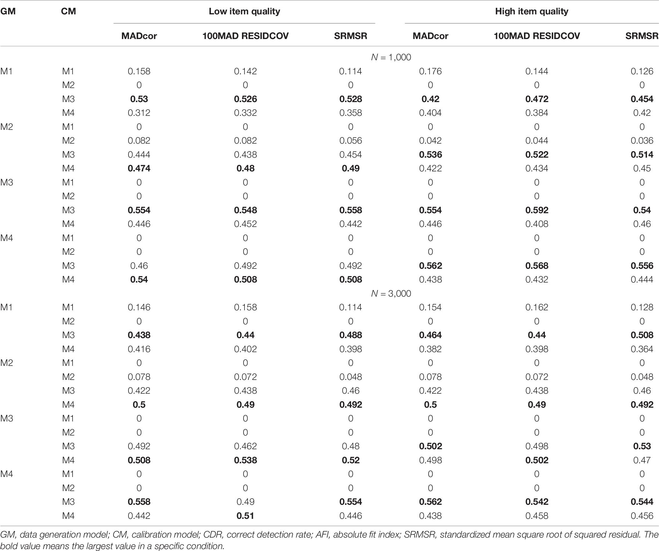
Table 9. CDRs of AFIs for different models with linear attribute structures.
Real Data Illustration
Data Source
This example application is from the TIMSS 2007 eighth-grade mathematics assessment, which is from Booklet 1 that measured three attributes (Lee et al., 2013): Attribute 1 (α1): whole numbers and integers; Attribute 2 (α2): fractions, decimals, and percentages; and Attribute 3 (α3): data analysis and probability. There are 12 dichotomously scored items and one three-category item answered by 544 students from the United States.
The Qc-matrix based on the works by Lee et al. (2013) and Ma (2019) is presented in Figure 4. According to general knowledge about numeric, α2 cannot be the prerequisite of α1. Hence, including the non-hierarchical attribute structure (#structure = 1), 11 different attribute structures are analyzed. The detailed DAGs of different hierarchical attribute structures are shown in Table 10. Without loss of generality, the GDINA model is chosen as the processing function in this section because, in simulation studies, we noticed that it is not easy to differentiate the SH-GDINA model from others. This dataset is analyzed using the GDINA R package (Ma and de la Torre, 2020).
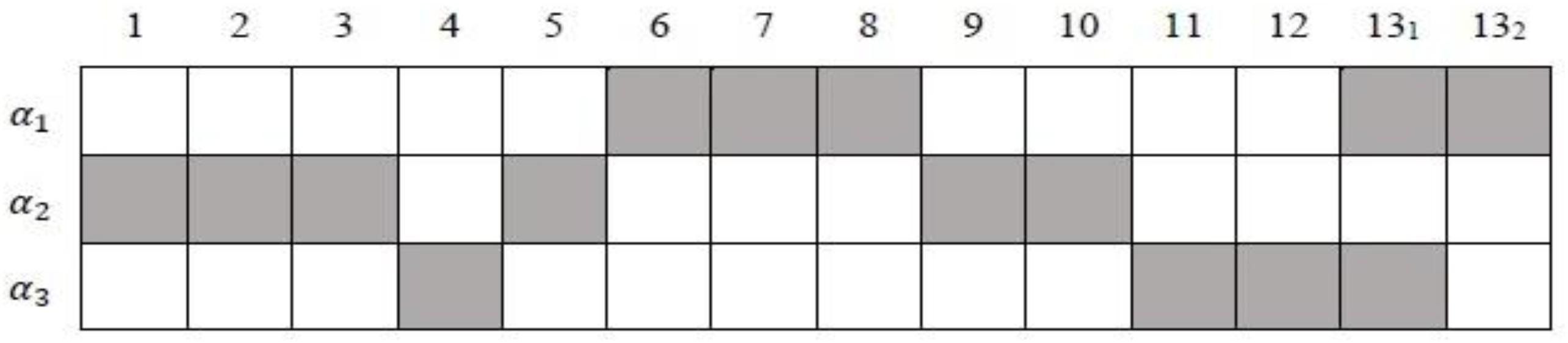
Figure 4. The Qc-matrix for Booklet 1 data from TIMSS 2007. 131 and 132 denote the 1st and 2nd tasks of item 13, respectively.
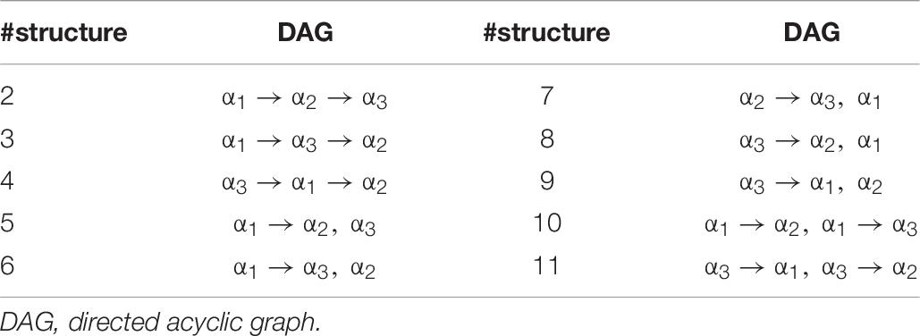
Table 10. Summary of hierarchical attribute structures.
Results
Table 11 shows the comparison among different structures using both AFIs and RFIs. The smallest values are in boldface. Different indices performed similarly to assess model-data fit that is because most of the items required only one attribute. From an item-level perspective, if only one attribute is required by one item, there is no difference among candidate models with different attribute structures.
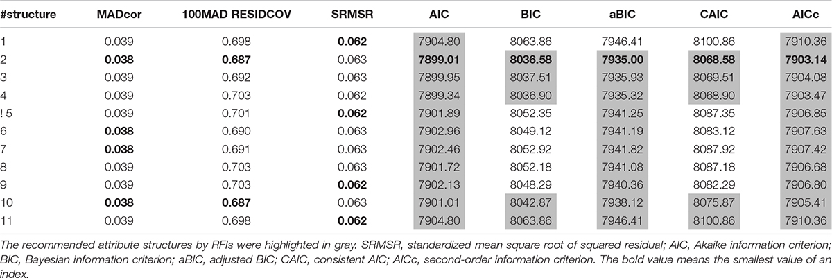
Table 11. Model fit indices of SH-GDINA models for TIMSS data.
On the other hand, Wang and Lu (2020) proposed two predetermined cutoff values (i.e., 0.025 and 0.05) of estimated proportions of latent classes to identify the labels for estimated latent classes. The estimated proportions of latent classes were shown in Table 12. All estimated proportions of (000), (100), (001), and (111) were larger than 0.025, and except (000) and (111), only (001) modeled using 4th structure had an estimated proportion larger than 0.05. It is not enough to distinguish different structures, which may be because the sample size of this dataset was small.
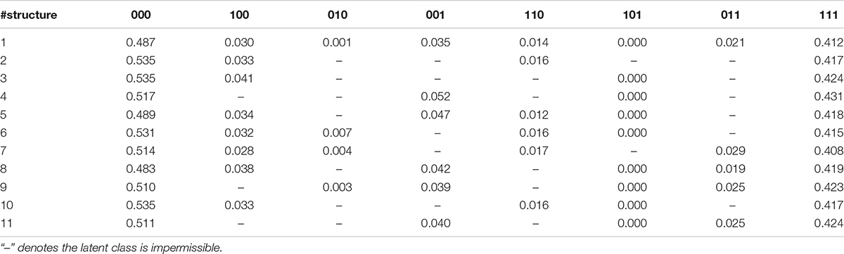
Table 12. Summary of estimated proportion of each latent class.
Conclusion
In order to avoid possible misleading conclusion, model-data fit must be thoroughly assessed before drawing the model-based inference. Although there are abundant research examining model fit assessment for CDMs, there is a lack of an effective guidance on how to deal with polytomously scored items with hierarchical attribute structures, and the aim of the present study is to fill in this gap. In this paper, we developed a sequential hierarchical cognitive diagnostic model to handle polytomous response data with hierarchical attribute structures and further evaluated model-data fit using both absolute fit indices and relative fit indices.
Across all simulation conditions, the SH-CDM can be recovered well, and aBIC and AICc are recommended for the SH-CDMs due to their high CDRs and acceptable distinguishable proportions. To distinguish different attribute structures for SH-GDINA models, RFIs outperform AFIs. Furthermore, AFIs used in this study are inappropriate to differentiate processing functions of the SH-CDM.
This study was the first attempt at assessing global-level fit of hierarchical CDMs and polytomous response data. However, the results are limited to SH-CDMs using the same condensation rules; future research pertaining to mixture measurement model and different condensation rules for different tasks in one item should be expanded to enhance the practicability of SH-CDMs. Also, it is necessary to extend the study to deal with sparse Q-matrix with large K. In addition, local-level (i.e., item-level) fit should be further examined to complement global fit analysis. On the other hand, as smaller values (close to zero) of AFIs indicate a good model-data fit, it would be worthwhile to identify the corresponding cutoff values using the resampling technique.
Data Availability Statement
Publicly available datasets were analyzed in this study. This data can be found here: https://timss.bc.edu/TIMSS2007/idb_ug.html.
Author Contributions
XZ provided original thoughts and completed the writing of this article. JW provided key technical support. Both authors contributed to the article and approved the submitted version.
Funding
This research was supported by the Fundamental Research Funds for the Central Universities (Grant 2412020QD004) and the Key Laboratory of Applied Statistics of MOE.
Conflict of Interest
The authors declare that the research was conducted in the absence of any commercial or financial relationships that could be construed as a potential conflict of interest.
Supplementary Material
The Supplementary Material for this article can be found online at: https://www.frontiersin.org/articles/10.3389/fpsyg.2020.579018/full#supplementary-material
Footnotes
- ^ A simulation check has been done to test the equivalence using the GDINA package; results indicated there was no significant difference between the identity link and the logit link.
References
Akaike, H. (1974). A new look at the statistical model identification. IEEE Trans. Autom. Control 19, 716–723. doi: 10.1109/tac.1974.1100705
Bozdogan, H. (1987). Model selection and Akaike’s information criterion (AIC): the general theory and its analytical extensions. Psychometrika 52, 345–370. doi: 10.1007/bf02294361
Burnham, K. P., and Anderson, D. R. (2002). Model Selection and Multimodel Inference: A Practical Information-Theoretic Approach. New York, NY: Springer.
Chen, J., de la Torre, J., and Zhang, Z. (2013). Relative and absolute fit evaluation in cognitive diagnosis modeling. J. Educ. Measur. 50, 123–140. doi: 10.1111/j.1745-3984.2012.00185.x
Culpepper, S. A. (2019). An exploratory diagnostic model for ordinal responses with binary attributes: identifiability and estimation. Psychometrika 84, 921–940. doi: 10.1007/s11336-019-09683-4
de la Torre, J. (2010). The partial-credit DINA model. Paper Presented at the International Meeting of the Psychometric Society, Athens, GA.
de la Torre, J. (2011). The generalized DINA model framework. Psychometrika 76, 179–199. doi: 10.1007/s11336-011-9207-7
DiBello, L. V., Roussos, L. A., and Stout, W. F. (2007). “Review of cognitively diagnostic assessment and a summary of psychometric models,” in Handbook of Statistics, Vol. 26, eds C. R. Rao and S. Sinharay (Amsterdam: Elsevier), 979–1030. doi: 10.1016/s0169-7161(06)26031-0
Gierl, M. J., Leighton, J. P., and Hunka, S. M. (2007). “Using the attribute hierarchy method to make diagnostic inferences about respondents’ cognitive skills,” in Cognitive Diagnostic Assessment for Education: Theory and Applications, eds J. P. Leighton and M. J. Gierl (Cambridge: Cambridge University Press), 242–274. doi: 10.1017/cbo9780511611186.009
Gu, Y., and Xu, G. (2019). Identification and estimation of hierarchical latent attribute models. arXiv [Preprint], Available online at: https://arxiv.org/abs/1906.07869v1 (accessed July 5, 2020).
Haertel, E. H. (1989). Using restricted latent class models to map the skill structure of achievement items. J. Educ. Measur. 26, 301–321. doi: 10.1111/j.1745-3984.1989.tb00336.x
Han, Z., and Johnson, M. S. (2019). “Global-and item-level model fit indices,” in Handbook of Diagnostic Classification Models, eds M. von Davier and Y. S. Lee (Cham: Springer), 265–285. doi: 10.1007/978-3-030-05584-4_13
Hansen, M. (2013). Hierarchical Item Response Models for Cognitive Diagnosis, Doctoral thesis, University of California, Los Angeles, CA.
Henson, R. A., Templin, J. L., and Willse, J. T. (2009). Defining a family of cognitive diagnosis models using log-linear models with latent variables. Psychometrika 74, 191–210. doi: 10.1007/s11336-008-9089-5
Hu, J., Miller, M. D., Huggins-Manley, A. C., and Chen, Y. H. (2016). Evaluation of model fit in cognitive diagnosis models. Intern. J. Test. 16, 119–141. doi: 10.1080/15305058.2015.1133627
Junker, B. W., and Sijtsma, K. (2001). Cognitive assessment models with few assumptions, and connections with nonparametric item response theory. Appl. Psychol. Measur. 25, 258–272. doi: 10.1177/01466210122032064
Lee, Y.-S., Johnson, M. S., Park, J. Y., Sachdeva, R., Zhang, J., and Waldman, M. (2013). A MDS Approach for investigating student’s cognitive weakness and strength on the TIMSS 2007 mathematics assessment. Paper Presented at the Annual Meeting of the American Educational Research Association, San Francisco, CA.
Lei, P. W., and Li, H. (2016). Performance of fit indices in choosing correct cognitive diagnostic models and Q-matrices. Appl. Psychol. Measur. 40, 405–417. doi: 10.1177/0146621616647954
Leighton, J., and Gierl, M. (2007). Cognitive Diagnostic Assessment for Education: Theory and Applications. Cambridge: Cambridge University Press.
Lim, Y. S., and Drasgow, F. (2019). Conditional independence and dimensionality of cognitive diagnostic models: a test for model fit. J. Classif. 36, 295–305. doi: 10.1007/s00357-018-9287-5
Liu, R., and Jiang, Z. (2020). A general diagnostic classification model for rating scales. Behav. Res. Methods 52, 422–439. doi: 10.3758/s13428-019-01239-9
Ma, W. (2017). A Sequential Cognitive Diagnosis Model for Graded Response: Model Development, Q-Matrix Validation, and Model Comparison. Doctoral thesis, Rutgers University-School of Graduate Studies, New Brunswick, NJ.
Ma, W. (2019). A diagnostic tree model for polytomous responses with multiple strategies. Br. J. Math. Statist. Psychol. 72, 61–82. doi: 10.1111/bmsp.12137
Ma, W. (2020). Evaluating the fit of sequential G-DINA model using limited-information measures. Appl. Psychol. Measur. 44, 167–181. doi: 10.1177/0146621619843829
Ma, W., and de la Torre, J. (2016). A sequential cognitive diagnosis model for polytomous responses. Br. J. Math. Statist. Psychol. 69, 253–275. doi: 10.1111/bmsp.12070
Ma, W., and de la Torre, J. (2019). Category-level model selection for the sequential G-DINA model. J. Educ. Behav. Statist. 44, 45–77. doi: 10.3102/1076998618792484
Ma, W., and de la Torre, J. (2020). GDINA: an R package for cognitive diagnosis modeling. J. Statist. Softw. 93, 1–26. doi: 10.14689/ejer.2019.80.9
Maydeu-Olivares, A. (2013). Goodness-of-fit assessment of item response theory models (with discussion). Measur. Interdiscipl. Res. Perspect. 11, 71–137. doi: 10.1080/15366367.2013.831680
McDonald, R. P., and Mok, M. M.-C. (1995). Goodness of fit in item response models. Multiv. Behav. Res. 30, 23–40. doi: 10.1207/s15327906mbr3001_2
Rupp, A. A., Templin, J., and Henson, R. A. (2010). Diagnostic Measurement: Theory, Methods, and Applications. New York, NY: Guilford Press.
Schwarz, G. (1978). Estimating the dimension of a model. Ann. Statist. 6, 461–464. doi: 10.1214/aos/1176344136
Sclove, L. (1987). Application of model-selection criteria to some problems in multivariate analysis. Psychometrika 52, 333–343. doi: 10.1007/bf02294360
Sen, S., and Bradshaw, L. (2017). Comparison of relative fit indices for diagnostic model selection. Appl. Psychol. Measur. 41, 422–438. doi: 10.1177/0146621617695521
Sinharay, S., and Almond, R. G. (2007). Assessing fit of cognitive diagnostic models a case study. Educ. Psychol. Measur. 67, 239–257. doi: 10.1177/0013164406292025
Sugiura, N. (1978). Further analysis of the data by Akaike’s information criterion and the finite corrections. Commun. Statist. Theor. Methods A 7, 13–26. doi: 10.1080/03610927808827599
Templin, J., and Bradshaw, L. (2013). Measuring the reliability of diagnostic classification model examinee estimates. J. Classific. 30, 251–275. doi: 10.1007/s00357-013-9129-4
Templin, J., and Bradshaw, L. (2014). Hierarchical diagnostic classification models: a family of models for estimating and testing attribute hierarchies. Psychometrika 79, 317–339. doi: 10.1007/s11336-013-9362-0
Templin, J. L., and Henson, R. A. (2006). Measurement of psychological disorders using cognitive diagnosis models. Psychol. Methods 11, 287–305. doi: 10.1037/1082-989x.11.3.287
Templin, J. L., Henson, R. A., Rupp, A. A., Jang, E., and Ahmed, M. (2008). Cognitive diagnosis models for nominal response data. Paper Presented at the Annual Meeting of the National Council on Measurement in Education, New York, NY.
Tutz, G. (1997). “Sequential models for ordered responses,” in Handbook of modern item response theory, eds W. J. van der Linden and R. K. Hambleton (New York, NY: Springer), 139–152. doi: 10.1007/978-1-4757-2691-6_8
von Davier, M. (2008). A general diagnostic model applied to language testing data. Br. J. Math. Statist. Psychol. 61, 287–307. doi: 10.1348/000711007x193957
von Davier, M., and Lee, Y. S. (2019). Handbook of Diagnostic Classification Models. Cham: Springer International Publishing.
Wang, C., and Lu, J. (2020). Learning attribute hierarchies from data: two exploratory approaches. J. Educ. Behav. Statist. [Epub ahead of print].
Keywords: sequential hierarchical cognitive diagnostic model, polytomous response data, attribute hierarchy, processing function, model fit
Citation: Zhang X and Wang J (2020) On the Sequential Hierarchical Cognitive Diagnostic Model. Front. Psychol. 11:579018. doi: 10.3389/fpsyg.2020.579018
Received: 01 July 2020; Accepted: 04 September 2020;
Published: 07 October 2020.
Edited by:
Liu Yanlou, Qufu Normal University, ChinaReviewed by:
Peida Zhan, Zhejiang Normal University, ChinaWenchao Ma, University of Alabama, United States
Copyright © 2020 Zhang and Wang. This is an open-access article distributed under the terms of the Creative Commons Attribution License (CC BY). The use, distribution or reproduction in other forums is permitted, provided the original author(s) and the copyright owner(s) are credited and that the original publication in this journal is cited, in accordance with accepted academic practice. No use, distribution or reproduction is permitted which does not comply with these terms.
*Correspondence: Juntao Wang, d2FuZ2p0NTY2QG5lbnUuZWR1LmNu