Albertson (Alb) spectral radii and Albertson (Alb) energies of graph operation

1 Introduction

Let G be a simple undirected connected regular graph with the vertex set V(G) = {v₁, v₂, … , v_z} and edge set E(G). If v_k and v_l are two nearby vertices of graph G, then v_kv_l is used to refer to the edge that connects them. We conventionally writes the vertex degree d_k related to the vertex v_k ∈ V(G) that represent total counting of edges end at a vertex v_k of a graph. The adjacency matrix for the graph G is a square matrix denoted as A(G) = Adj(G) = [a_kl], in which [a_kl] = 1 when two vertices v_k and v_l are adjacent otherwise it defines to be as zero, mathematically it can be formulated as $A(G)=\left\{\begin{array}{cc}1\hfill & \text{if}{v}_k\sim v_l,\hfill \\ 0\hfill & \text{elsewhere}.\hfill \end{array}\right.$. The adjacency eigenvalues of G labelled as $(\acute{{\gamma }_1},\acute{{\gamma }_2},\dots ,\acute{{\gamma }_z})$ are the eigenvalues of A(G). With the help of these eigenvalues we define the spectrum of related graph G (Cvetković et al., 2009) and then concluded their energy.

The graph energy is one of the very few mathematical ideas which are chemically motivated into the modern subject of mathematics. Additionally, Graph theory encompasses various invariants that are significant for understanding the properties of a graph. Among these, the energy and spectral radius hold particular importance. Furthermore, the concept of graph energy, denoted as ɛ(G), was initially introduced by Gutman in 1978 (Gutman, 1978). However, Initially, this notion was met with skepticism and was explored by only a limited group of scientists due to its unconventional nature. Nevertheless, it wasn’t until the year 2000 that mathematicians truly embraced this concept. At present, the idea of graph energy has gained substantial recognition due to its wide-ranging applications across diverse industries. Consequently, there is a surge of interest in this field, leading to the constant emergence of graph energy and fundamental algebraic identities. Notably, graph energy captures the graphical characteristic, while the spectral radius of a graph represents the largest absolute eigenvalue among all the eigenvalues of its adjacency matrix, denoted by the notation ℘(G). Moreover, these mathematical tools have found several applications in algebraic graph theory (Zhang et al., 2022). Both of these tools, i.e., the energy and spectral radius, play pivotal roles in comprehending the structural properties and behavior of graphs across various disciplines. They offer valuable insights into a graph’s connectivity, stability, expansion, and spread dynamics, making them indispensable for the analysis and characterization of graphs in different contexts.

There is a considerable and visible connection between chemistry and graph theory. Specifically in graph theory, the degree of a molecular graph vertex corresponds to the valency of an atom. Moreover, A variety of topological indices have been built on the product of the degrees d_k and d_l of the terminal vertices k and l of the edge (chemical bond) kl, which has attracted the interest of mathematical chemists. In recent decades, topological indices have undergone extensive research in a number of fields, including mathematics (Gutman and Polansky, 2012; Janezic et al., 2015), physics (Labanowski et al., 1991), biology (Bajorath and Bajorath, 2011). Notably, they have found applications especially in chemical disciplines (Klein et al., 1992; Trinajstić and Nikolić, 2000), such as chemical documentation, isomer discrimination, study of molecular complexity, and other related fields like QSAR and QSPR, drug design, database choice, etc. A topological index (Gutman, 2013) is a numerical value intrinsically tied to a graph, serving as a fundamental characterizer of the graph’s topology while retaining its consistency through graph transformations. Within the realm of chemical graph theory, degree-based topological indices assume a paramount role and hold immense significant. Topological indices and graph invariants based on vertex degree and the distance between vertices are commonly serve as indispensable tools in characterizing molecular graphs. In the work of Gao et al. (2016a); Gao et al. (2016b) several noteworthy findings on topological indices of chemical graphs have emerged. These techniques establish a profound link between a molecule’s structure attributes and its properties, thereby enabling the predictions of biological activity for chemical compounds, and contributing to the development of various chemical applications. Among these indices, Wiener index, the pioneer and extensively researched topological index, has accumulate significant attention in terms of both theoretical standpoint and practical applications. Similarly, the Zagreb indices, which are degree-based topological indices, have been the subject of extensive exploration and were originally introduced by Gutman and Trinajsti$\acute{c}$ (Gutman and Trinajstić, 1972). These indices provide valuable insights into the graph’s overall structure and the characteristics of its vertices. Specifically, the first Zagreb index, denoted as ZI₁(G), is defined as the sum of the squares of the vertex degrees within a molecular graph. On the other hand, the second Zagreb index ZI₂(G) corresponds to the sum of the product of the vertex degrees of pairs of adjacent vertices. In a mathematical approach, this relationship is expressed as follow: $Z{I}_1(G)={\sum }_{v\in V(G)}{d}_G^2(v)={\sum }_{kl\in E(G)}(d_G(k)+d_G(l))$ and is ZI₂(G) = ∑_kl∈E(G)(d_G(k)d_G(l)). Moving on, M.O. Albertson (Albertson, 1997) introduced Albertson matrix, which contains the entries ∣d_G(k) − d_G(l)∣ when two vertices v_k and v_l are adjacent (i.e., v_k ∼ v_l) and zeroes elsewhere. It is occasionally famed as the Albertson Index (Gutman et al., 2005) and referred to as the third zagreb index in a recent work (Fath-Tabar, 2011). The topological indicator known as the Albertson index serves to describe the structural characteristic of molecule, particulary in the context of quantitative structure activity relationship (QSAR) research in chemistry. QSAR is a technique employed for predicting a chemical compound’s biological activity or characteristic based on its molecular structure. In essence, it assesses the connectedness, interconnectedness, and robustness of a graph. It also gauges the effectiveness of information or signal transmission within the network and the degree of connectedness between vertices. It’s worth noting that a graph with a higher index value tends to be more robust and resilient.

The significance of energy and spectral radii of a graph extends across diverse fields. In the realm of social network analysis, energy serves as a crucial metric for measuring network stability, while spectral radius highlights influential nodes within the network. Likewise, in the domain of electrical circuit analysis, graphs play a pivotal role in illustrating circuit components and their interconnections. The energy of a graph becomes a meaningful measure, reflecting the total energy or power dissipation within an electrical circuit, while spectral radius aids stability analysis and the determination of maximum gain or amplification within feedback systems. Furthermore, the spectral radius determines visual patterns in the realm of image processing while energy gauges pixel cohesiveness. Beyond this, the energy of a graph finds utility in epidemiology and disease spread modeling, where it can illustrate the potential for disease transmission between individuals. A lower energy value may indicate a situation that is less contagious, providing valuable insights for disease control strategies. On the other hand, the spectral radius plays a key role in the calculation of the basic reproduction number (R₀) in epidemic models, with a larger spectral radius suggesting a higher potential for an outbreak. In addition to these applications, recommender systems utilize energy to gauge user-item compatibility and the spectral radius to identify influential factors. These metrics offer valuable across a spectrum of systems, including social networks, electrical circuits, and epidemiology, enhancing analysis and making predictions more accurate.

The energy and spectral radii of the original graph and those of the splitting and shadow graphs have recently been found to have a substantial relationship. The dimer problem and Huckle′s theory, which serve as examples of how graph spectra are used in statistical physics and chemistry, have also been used in this study to make general findings and emphasise this application. Notably, the utilization of graph spectra in these domains is well-documented, as evidenced by the work of Cvetkovic et al. (1980). Furthermore, Bilal et al. made significant strides in uncovering the significance correlation between the ISI energies and the ISI spectral radii of the base graph, as well as those of the splitting and shadow graphs, in their recent research (Ahmad et al., 2023). These findings illuminate the structural characteristics of the graph and underscore the interdependence of these measurements. In a complementary vein, another recent study by Ahmad and Munir (2022a) offers noteworthy insights into the strong relation between the ABC energies and ABC spectral radii of the base graph, as well as those of the splitting and shadow graphs. Bilal et al. in his recent study (Ahmad and Munir, 2022b) unveiled some valueable relationship concerning the randic and reciprocal randic energy and spectral radii of original graph and in correspondence to splitting and shadow graphs. The references (Yu et al., 2004) serve as valuable resources for insights on spectral radii. In (Shao et al., 2021), Shao et al. made a notable discovery regarding the minimum augmented Zagreb energy of trees. Additionally, researchers such as Horn et al. (Horn and Johnson, 1991) and Gatmacher (Gantmacher, 1959) delved into matrix analysis in relation to graph energies, further expanding our understanding of this field. Xavier et al. (2022) described energy of Cartesian product of graph nework. Samir et al. (Vaidya and Popat, 2017a) developed one-splitting and two-shadow graphs of a simple connected graph, revealing that these graphs’ adjacency energies are constant multiples of the energies of the original graph. Expanding on these ideas, Samir et al. (Vaidya and Popat, 2017b) contributed significant findings related to adjacency energies. In Liu et al. (2019) explored the distance and adjacency energy of multiple-level wheel networks, adding another layer of depth to the study of graph energies. The signless Laplacian and Laplacian energies, as well as their spectra, were established by Chu et al. (2020) by means of multi-step wheels. A remarable work on graph energy and its uses was published by I. Gutman et al. in (Li et al., 2012), which included information on more than a hundred different types of graph energies and their applications in various fields. Numerous graph energies have applications in crystallography (Yuge, 2018), as well as in the theory of macromolecules (Pražnikar et al., 2019), biology (Giuliani et al., 2014), protein sequencing (Wu et al., 2015; Yu et al., 2017), air travel problems (Jiang et al., 2016), and spacecraft architecture (Pugliese and Nilchiani, 2017).

In Section 2, we delve into the core concepts centered around the Albertson Estrada (Alb) energy and spectral radii of splitting and shadow of regular graphs. Our exploration commences by examining regular graph G and formulating general results employing the splitting and shadow graph invariant. Subsequently, we extrapolate from these general findings to obtain specific results that pertain to various regular graph types, including cycle(C_z) graphs, complete graphs(K_z), complete bipartite(K_z,z) graphs, etc. The Alb spectral radius and energy of the splitting graph and shadow graph come under scrutiny in Section 3.

2 Preliminaries

In this section, we will lay out the essential ideas and present pertinent background data related to our key discoveries. Spectral graph theory plays a key role in different applications across different areas ranging from computer science, networking, chemistry, physics, as well as almost all areas of mathematics. The application of spectral graph theory in chemistry is highly significant, particularly in constructing a connection between graph eigenvalues and the levels of energy of molecular orbital associated with $\acute{\pi }$-electrons in conjugated hydrocarbons. In the context of the H$\ddot{u}$ckel Molecular Orbital $(\acute{H}MO)$ approximation (Zimmerman, 2011), the levels of energy of $\acute{\pi }$-electrons in conjugated hydrocarbon molecules can be more closely related with the eigenvalues of a chemical graph referred to as the molecular graph. To provide a tangible example, consider the chemical structure of Perylene depicted in Figure 1, which serve as a representative conjugated hydrocarbon with the formula $\acute{H}$. It consists of a total of 20-carbon atoms, it exhibits a graph with z = 20.

FIGURE 1

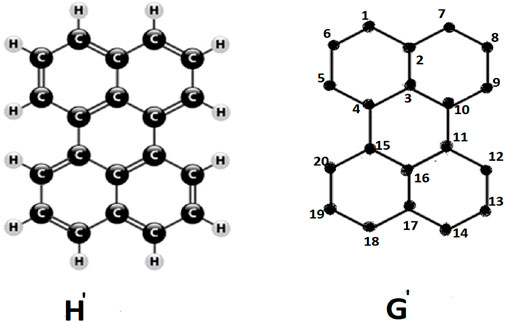
FIGURE 1. Perylene H′ and it’s molecular graph G′.

Perylene, H′, is an example of a conjugated hydrocarbon, characterized by its carbon atom structure illustrate as chemical graph G′ in above figure. The vertices of the graph G′ are denoted as 1, 2, … , 20, which represent the carbon atoms in the chemical formula H′. In the H$\ddot{u}$ckel Molecular Orbital $(\acute{H}MO)$ model, the wave functions of a conjugated hydrocarbon with a specified number of carbon atoms, indicated as ’z,’ are represented as a linear combination within an z-dimensional space made up of orthogonal basis functions. Simultaneously, Hamiltonian Matrix, which is a square matrix of order z by z, is defined as:

$\acute{H_{ij}}=\left\{\begin{array}{cc}\gamma ,\hfill & \text{If}\mathrm{i}=\mathrm{j},\hfill \\ \kappa ,\hfill & \text{If\hspace{0.17em}there\hspace{0.17em}is\hspace{0.17em}a\hspace{0.17em}chemical\hspace{0.17em}bond\hspace{0.17em}between\hspace{0.17em}atoms}\mathrm{i}\text{and}\mathrm{j},\hfill \\ 0,\hfill & \text{If\hspace{0.17em}there\hspace{0.17em}is\hspace{0.17em}no\hspace{0.17em}chemical\hspace{0.17em}bond\hspace{0.17em}between\hspace{0.17em}atoms}\mathrm{i}\text{and}\mathrm{j},\hfill \end{array}\right.$

where the parameters γ and κ are constants. As a demonstration, the $(\acute{H}MO)$ Hamiltonian matrix related to Perylene is:

$\acute{H}=\left[\begin{array}{cccccccccccccccccccc}\hfill \gamma \hfill & \hfill \kappa \hfill & \hfill 0\hfill & \hfill 0\hfill & \hfill 0\hfill & \hfill \kappa \hfill & \hfill 0\hfill & \hfill 0\hfill & \hfill 0\hfill & \hfill 0\hfill & \hfill 0\hfill & \hfill 0\hfill & \hfill 0\hfill & \hfill 0\hfill & \hfill 0\hfill & \hfill 0\hfill & \hfill 0\hfill & \hfill 0\hfill & \hfill 0\hfill & \hfill 0\hfill \\ \hfill \kappa \hfill & \hfill \gamma \hfill & \hfill \kappa \hfill & \hfill 0\hfill & \hfill 0\hfill & \hfill 0\hfill & \hfill \kappa \hfill & \hfill 0\hfill & \hfill 0\hfill & \hfill 0\hfill & \hfill 0\hfill & \hfill 0\hfill & \hfill 0\hfill & \hfill 0\hfill & \hfill 0\hfill & \hfill 0\hfill & \hfill 0\hfill & \hfill 0\hfill & \hfill 0\hfill & \hfill 0\hfill \\ \hfill 0\hfill & \hfill \kappa \hfill & \hfill \gamma \hfill & \hfill \kappa \hfill & \hfill 0\hfill & \hfill 0\hfill & \hfill 0\hfill & \hfill 0\hfill & \hfill 0\hfill & \hfill \kappa \hfill & \hfill 0\hfill & \hfill 0\hfill & \hfill 0\hfill & \hfill 0\hfill & \hfill 0\hfill & \hfill 0\hfill & \hfill 0\hfill & \hfill 0\hfill & \hfill 0\hfill & \hfill 0\hfill \\ \hfill 0\hfill & \hfill 0\hfill & \hfill \kappa \hfill & \hfill \gamma \hfill & \hfill \kappa \hfill & \hfill 0\hfill & \hfill 0\hfill & \hfill 0\hfill & \hfill 0\hfill & \hfill 0\hfill & \hfill 0\hfill & \hfill 0\hfill & \hfill 0\hfill & \hfill 0\hfill & \hfill \kappa \hfill & \hfill 0\hfill & \hfill 0\hfill & \hfill 0\hfill & \hfill 0\hfill & \hfill 0\hfill \\ \hfill 0\hfill & \hfill 0\hfill & \hfill 0\hfill & \hfill \kappa \hfill & \hfill \gamma \hfill & \hfill \kappa \hfill & \hfill 0\hfill & \hfill 0\hfill & \hfill 0\hfill & \hfill 0\hfill & \hfill 0\hfill & \hfill 0\hfill & \hfill 0\hfill & \hfill 0\hfill & \hfill 0\hfill & \hfill 0\hfill & \hfill 0\hfill & \hfill 0\hfill & \hfill 0\hfill & \hfill 0\hfill \\ \hfill \kappa \hfill & \hfill 0\hfill & \hfill 0\hfill & \hfill 0\hfill & \hfill \kappa \hfill & \hfill \gamma \hfill & \hfill 0\hfill & \hfill 0\hfill & \hfill 0\hfill & \hfill 0\hfill & \hfill 0\hfill & \hfill 0\hfill & \hfill 0\hfill & \hfill 0\hfill & \hfill 0\hfill & \hfill 0\hfill & \hfill 0\hfill & \hfill 0\hfill & \hfill 0\hfill & \hfill 0\hfill \\ \hfill 0\hfill & \hfill \kappa \hfill & \hfill 0\hfill & \hfill 0\hfill & \hfill 0\hfill & \hfill 0\hfill & \hfill \gamma \hfill & \hfill \kappa \hfill & \hfill 0\hfill & \hfill 0\hfill & \hfill 0\hfill & \hfill 0\hfill & \hfill 0\hfill & \hfill 0\hfill & \hfill 0\hfill & \hfill 0\hfill & \hfill 0\hfill & \hfill 0\hfill & \hfill 0\hfill & \hfill 0\hfill \\ \hfill 0\hfill & \hfill 0\hfill & \hfill 0\hfill & \hfill 0\hfill & \hfill 0\hfill & \hfill 0\hfill & \hfill \kappa \hfill & \hfill \gamma \hfill & \hfill \kappa \hfill & \hfill 0\hfill & \hfill 0\hfill & \hfill 0\hfill & \hfill 0\hfill & \hfill 0\hfill & \hfill 0\hfill & \hfill 0\hfill & \hfill 0\hfill & \hfill 0\hfill & \hfill 0\hfill & \hfill 0\hfill \\ \hfill 0\hfill & \hfill 0\hfill & \hfill 0\hfill & \hfill 0\hfill & \hfill 0\hfill & \hfill 0\hfill & \hfill 0\hfill & \hfill \kappa \hfill & \hfill \gamma \hfill & \hfill \kappa \hfill & \hfill 0\hfill & \hfill 0\hfill & \hfill 0\hfill & \hfill 0\hfill & \hfill 0\hfill & \hfill 0\hfill & \hfill 0\hfill & \hfill 0\hfill & \hfill 0\hfill & \hfill 0\hfill \\ \hfill 0\hfill & \hfill 0\hfill & \hfill \kappa \hfill & \hfill 0\hfill & \hfill 0\hfill & \hfill 0\hfill & \hfill 0\hfill & \hfill 0\hfill & \hfill \kappa \hfill & \hfill \gamma \hfill & \hfill \kappa \hfill & \hfill 0\hfill & \hfill 0\hfill & \hfill 0\hfill & \hfill 0\hfill & \hfill 0\hfill & \hfill 0\hfill & \hfill 0\hfill & \hfill 0\hfill & \hfill 0\hfill \\ \hfill 0\hfill & \hfill 0\hfill & \hfill 0\hfill & \hfill 0\hfill & \hfill 0\hfill & \hfill 0\hfill & \hfill 0\hfill & \hfill 0\hfill & \hfill 0\hfill & \hfill \kappa \hfill & \hfill \gamma \hfill & \hfill \kappa \hfill & \hfill 0\hfill & \hfill 0\hfill & \hfill 0\hfill & \hfill \kappa \hfill & \hfill 0\hfill & \hfill 0\hfill & \hfill 0\hfill & \hfill 0\hfill \\ \hfill 0\hfill & \hfill 0\hfill & \hfill 0\hfill & \hfill 0\hfill & \hfill 0\hfill & \hfill 0\hfill & \hfill 0\hfill & \hfill 0\hfill & \hfill 0\hfill & \hfill 0\hfill & \hfill \kappa \hfill & \hfill \gamma \hfill & \hfill \kappa \hfill & \hfill 0\hfill & \hfill 0\hfill & \hfill 0\hfill & \hfill 0\hfill & \hfill 0\hfill & \hfill 0\hfill & \hfill 0\hfill \\ \hfill 0\hfill & \hfill 0\hfill & \hfill 0\hfill & \hfill 0\hfill & \hfill 0\hfill & \hfill 0\hfill & \hfill 0\hfill & \hfill 0\hfill & \hfill 0\hfill & \hfill 0\hfill & \hfill 0\hfill & \hfill \kappa \hfill & \hfill \gamma \hfill & \hfill \kappa \hfill & \hfill 0\hfill & \hfill 0\hfill & \hfill 0\hfill & \hfill 0\hfill & \hfill 0\hfill & \hfill 0\hfill \\ \hfill 0\hfill & \hfill 0\hfill & \hfill 0\hfill & \hfill 0\hfill & \hfill 0\hfill & \hfill 0\hfill & \hfill 0\hfill & \hfill 0\hfill & \hfill 0\hfill & \hfill 0\hfill & \hfill 0\hfill & \hfill 0\hfill & \hfill \kappa \hfill & \hfill \gamma \hfill & \hfill 0\hfill & \hfill 0\hfill & \hfill \kappa \hfill & \hfill 0\hfill & \hfill 0\hfill & \hfill 0\hfill \\ \hfill 0\hfill & \hfill 0\hfill & \hfill 0\hfill & \hfill \kappa \hfill & \hfill 0\hfill & \hfill 0\hfill & \hfill 0\hfill & \hfill 0\hfill & \hfill 0\hfill & \hfill 0\hfill & \hfill 0\hfill & \hfill 0\hfill & \hfill 0\hfill & \hfill 0\hfill & \hfill \gamma \hfill & \hfill \kappa \hfill & \hfill 0\hfill & \hfill 0\hfill & \hfill 0\hfill & \hfill \kappa \hfill \\ \hfill 0\hfill & \hfill 0\hfill & \hfill 0\hfill & \hfill 0\hfill & \hfill 0\hfill & \hfill 0\hfill & \hfill 0\hfill & \hfill 0\hfill & \hfill 0\hfill & \hfill 0\hfill & \hfill \kappa \hfill & \hfill 0\hfill & \hfill 0\hfill & \hfill 0\hfill & \hfill \kappa \hfill & \hfill \gamma \hfill & \hfill \kappa \hfill & \hfill 0\hfill & \hfill 0\hfill & \hfill 0\hfill \\ \hfill 0\hfill & \hfill 0\hfill & \hfill 0\hfill & \hfill 0\hfill & \hfill 0\hfill & \hfill 0\hfill & \hfill 0\hfill & \hfill 0\hfill & \hfill 0\hfill & \hfill 0\hfill & \hfill 0\hfill & \hfill 0\hfill & \hfill 0\hfill & \hfill \kappa \hfill & \hfill 0\hfill & \hfill \kappa \hfill & \hfill \gamma \hfill & \hfill \kappa \hfill & \hfill 0\hfill & \hfill 0\hfill \\ \hfill 0\hfill & \hfill 0\hfill & \hfill 0\hfill & \hfill 0\hfill & \hfill 0\hfill & \hfill 0\hfill & \hfill 0\hfill & \hfill 0\hfill & \hfill 0\hfill & \hfill 0\hfill & \hfill 0\hfill & \hfill 0\hfill & \hfill 0\hfill & \hfill 0\hfill & \hfill 0\hfill & \hfill 0\hfill & \hfill \kappa \hfill & \hfill \gamma \hfill & \hfill \kappa \hfill & \hfill 0\hfill \\ \hfill 0\hfill & \hfill 0\hfill & \hfill 0\hfill & \hfill 0\hfill & \hfill 0\hfill & \hfill 0\hfill & \hfill 0\hfill & \hfill 0\hfill & \hfill 0\hfill & \hfill 0\hfill & \hfill 0\hfill & \hfill 0\hfill & \hfill 0\hfill & \hfill 0\hfill & \hfill 0\hfill & \hfill 0\hfill & \hfill 0\hfill & \hfill \kappa \hfill & \hfill \gamma \hfill & \hfill \kappa \hfill \\ \hfill 0\hfill & \hfill 0\hfill & \hfill 0\hfill & \hfill 0\hfill & \hfill 0\hfill & \hfill 0\hfill & \hfill 0\hfill & \hfill 0\hfill & \hfill 0\hfill & \hfill 0\hfill & \hfill 0\hfill & \hfill 0\hfill & \hfill 0\hfill & \hfill 0\hfill & \hfill \kappa \hfill & \hfill 0\hfill & \hfill 0\hfill & \hfill 0\hfill & \hfill \kappa \hfill & \hfill \gamma \hfill \end{array}\right].$

Based on the given example, it is clear that even in the overall scenario within the $(\acute{H}MO)$ model, it is necessary to address the eigenvalue-eigenvector dilemma of an approximate Hamiltonian matrix. This matrix follows a specific structure expressed as:

$\acute{H}=\gamma I_z+\kappa A\left(G^{\prime }\right)(2.1)$

Here, γ and κ represent specific constants, I_z denotes the z-dimensional unit matrix and the adjacency matrix of a specific graph G′ is signifies as A(G′) comprising the z vertices, which represents the carbon-atom framework of the underlying conjugated molecule. The energy levels of total $\acute{\pi }$-electron are determined by the respective eigenvalue of the adjacency matix of G′. By virtue of above equation, the energy levels ɛ_k associated with the $\acute{\pi }$-electrons exhibit a straightforward connection to the eigenvalues η_k of the graph G′.

${\epsilon }_k=\gamma +\kappa {\eta }_k;k=\mathrm{1,2}\cdots ,20.(2.2)$

Within the framework of the $\acute{H}MO$ approximation, the collective E of all $\acute{\pi }$-electrons illustrated as $E={\epsilon }_{\acute{\pi }}(G)={\sum }_{k=1}^z{g}_k{\epsilon }_k$. In this context, the term ’occupation number’ refers to g_k, which signifies the quantity associated with the given property. The main point to note is that the number of $\acute{\pi }$-electrons (denoted by z) in the conjugated hydrocarbons being studied is equal to the sum of individual counts (g₁ + g₂ + ⋯ + g_z). Consequently, this implies that $\epsilon (G)={\sum }_{k=1}^z\mid {\eta }_k\mid$.

Let [Alb(G)] = x_kl referred as Albertson matrix of the graph G specified in (Albertson, 1997) possessing entries,

$x_{kl}=\left\{\begin{array}{cc}|d_k-d_l|,\hfill & \text{if}{v}_k\text{and}{v}_l\text{are\hspace{0.17em}adjacent},\hfill \\ 0\hfill & \text{if}k=l,\hfill \\ 0\hfill & \text{elsewhere}.\hfill \end{array}\right.$

Here, the degrees of the vertices v_k and v_l are d_k and d_l respectively. Let eigenvalues of the Albertson matrix of the graph G are define as $\acute{{\xi }_1},\acute{{\xi }_2},\cdots \acute{{\xi }_z}$. The Alb eigenvalues makes up the Alb spectrum of the graph. If distinct eigenvalues $\acute{{\xi }_1},\acute{{\xi }_2},\cdots \acute{{\xi }_z}$ of Albertson of the graph G are define with multiplicities $\acute{m_1},\acute{m_2},\dots ,\acute{m_z}$, respectively, then

$spec\left(Alb\right)=\left(\begin{array}{cccc}\hfill \acute{{\xi }_1}\hfill & \hfill \acute{{\xi }_2}\hfill & \hfill \cdots \hfill & \hfill \acute{{\xi }_z}\hfill \\ \hfill \acute{m_1}\hfill & \hfill \acute{m_2}\hfill & \hfill \cdots \hfill & \hfill \acute{m_z}\hfill \end{array}\right).(2.3)$

With the help of this spectrum, Albertson (Alb) energy of a graph (G) is defined as

$Alb\epsilon \left(G\right)={\displaystyle \sum _{i=1}^z}\left|\begin{array}{c}\hfill \acute{{\xi }_i}\hfill \end{array}\right|.$

In Spectral graph theory, spectral radius stand together with graph energy symbolize as ℘Alb(G) and define as:

$\wp Alb\left(G\right)={\max }_{i=1}^z\left|\begin{array}{c}\hfill \acute{{\xi }_i}\hfill \end{array}\right|,$

Where $\acute{{\xi }_i}$ indicated as the eigenvalue of the Albertson matrix ranging from 1 ≤ i ≤ z. The following definition are crucial to our conclusions.

Definition 1.1 Splitting graph Spl_s(G) of a connected graph G is obtained by adding new s vertices to each vertex v of a graph G, making sure that every new vertex is connected to every vertex that is adjacent to v in the graph G.

Figures 2, 3 should the situation as in Defintion 1.1.

FIGURE 2

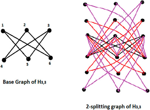
FIGURE 2. A base graph H(3,3) and it’s respective Spl₂(H(3,3)).

FIGURE 3

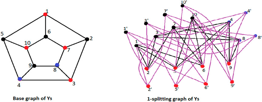
FIGURE 3. A base graph of (Y₅) and it’s associated Spl₁(Y₅).

Definition 1.2 Shadow graph Sh_s(G) of a connected graph G is established by taking s copies of G, say G₁, G₂, … , G_s then join each vertex u in G_i to the neighbours of the corresponding vertex v in G_j, 1 ≤ i, j ≤ s.

Figure 4 should the situation as in definition 1.2. (Neumaier, 1992) Let AϵR^m×n, BϵR^p×q. Then A⊗B is given by

$A\otimes B=\left(\begin{array}{cccc}\hfill a_{11}B\hfill & \hfill .\hfill & \hfill .\hfill & \hfill .a_{1n}B\hfill \\ \hfill .\hfill & \hfill .\hfill & \hfill .\hfill & \hfill .\hfill \\ \hfill .\hfill & \hfill .\hfill & \hfill .\hfill & \hfill .\hfill \\ \hfill .\hfill & \hfill .\hfill & \hfill .\hfill & \hfill .\hfill \\ \hfill a_{m1}B\hfill & \hfill .\hfill & \hfill .\hfill & \hfill .a_{mn}B\hfill \end{array}\right).$

Proposition 1.1 (Neumaier, 1992) Assuming that α is an eigenvalue of A and β is an eigenvalue of B, let’s write AϵM^m, BϵMⁿ. Then an eigenvalue of A ⊗ B is αβ.

FIGURE 4

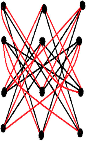
FIGURE 4. Sh₂(H_3,3), the 2-shadow graph of H_3,3.

3 Albertson energy and spectral radii of generalized splitting graphs

In this section, we compare the Albertson energies (Alb) and spectral radii of generalized splitting and shadow graph of a regular graph G with the corresponding Albertson energies (Alb) and spectral radii of its original graph. It is essential to emphasize that G denotes any k-regular graph.

Theorem 1. If a graph G is k-regular, then the Albertson energy for the generalized splitting of a regular graph is define as, $Alb\epsilon (Sp{l}_s(G))=Adj\epsilon (G)(2ks\sqrt{s})$.

Proof. Let G be a k regular graph with vertex set V(G) = {v₁, v₂, v₃, … , v_z} and Spl_s(G) be the splitting graph of graph G with vertex set V(Spl_s(G)) = {v₁₁, v₁₂, … , v_1z, v₂₁, v₂₂, … , v_2z, … , v_s1, v_s2, … , v_sz} ∪ V(G). Then Alb(Spl_s(G)) matrix can be written as follows

$Alb\left(Sp{l}_s\left(G\right)\right)={\left[\begin{array}{cccc}\hfill {\aleph }_1\hfill & \hfill {\aleph }_2\hfill & \hfill \dots \hfill & \hfill {\aleph }_2\hfill \\ \hfill {\aleph }_2\hfill & \hfill {\aleph }_1\hfill & \hfill \dots \hfill & \hfill {\aleph }_1\hfill \\ \hfill ⋮\hfill & \hfill ⋮\hfill & \hfill \ddots \hfill & \hfill ⋮\hfill \\ \hfill {\aleph }_2\hfill & \hfill {\aleph }_1\hfill & \hfill \cdots \hfill & \hfill {\aleph }_1\hfill \end{array}\right]}_{s+1},$

where the matrix ℵ₁ is defined by ℵ₁ = Alb(G), and the matrix ℵ₂ is defined by ℵ₂ = ksAdj(G).

$\begin{array}{ll}\hfill Alb\left(Sp{l}_s\left(G\right)\right)& ={\left[\begin{array}{cccc}\hfill Alb\left(G\right)\hfill & \hfill ksAdj\left(G\right)\hfill & \hfill \dots \hfill & \hfill ksAdj\left(G\right)\hfill \\ \hfill ksAdj\left(G\right)\hfill & \hfill Alb\left(G\right)\hfill & \hfill \dots \hfill & \hfill Alb\left(G\right)\hfill \\ \hfill ⋮\hfill & \hfill ⋮\hfill & \hfill \ddots \hfill & \hfill ⋮\hfill \\ \hfill ksAdj\left(G\right)\hfill & \hfill Alb\left(G\right)\hfill & \hfill \cdots \hfill & \hfill Alb\left(G\right)\hfill \end{array}\right]}_{s+1}\hfill \\ \hfill & ={\left[\begin{array}{cccc}\hfill Alb\left(G\right)+0Adj\left(G\right)\hfill & \hfill Alb\left(G\right)+ksAdj\left(G\right)\hfill & \hfill \dots \hfill & \hfill Alb\left(G\right)+ksAdj\left(G\right)\hfill \\ \hfill Alb\left(G\right)+ksAdj\left(G\right)\hfill & \hfill Alb\left(G\right)+0Adj\left(G\right)\hfill & \hfill \dots \hfill & \hfill Alb\left(G\right)+0Adj\left(G\right)\hfill \\ \hfill ⋮\hfill & \hfill ⋮\hfill & \hfill \ddots \hfill & \hfill ⋮\hfill \\ \hfill Alb\left(G\right)+ksAdj\left(G\right)\hfill & \hfill Alb\left(G\right)+0Adj\left(G\right)\hfill & \hfill \cdots \hfill & \hfill Alb\left(G\right)+0Adj\left(G\right)\hfill \end{array}\right]}_{s+1}\hfill \\ \hfill & ={\left[\begin{array}{ccc}\hfill Alb\left(G\right)\hfill & \hfill \dots \hfill & \hfill Alb\left(G\right)\hfill \\ \hfill ⋮\hfill & \hfill \ddots \hfill & \hfill ⋮\hfill \\ \hfill Alb\left(G\right)\hfill & \hfill \cdots \hfill & \hfill Alb\left(G\right)\hfill \end{array}\right]}_{s+1}+{\left[\begin{array}{cccc}\hfill 0Adj\left(G\right)\hfill & \hfill ksAdj\left(G\right)\hfill & \hfill \dots \hfill & \hfill ksAdj\left(G\right)\hfill \\ \hfill ksAdj\left(G\right)\hfill & \hfill 0Adj\left(G\right)\hfill & \hfill \dots \hfill & \hfill 0Adj\left(G\right)\hfill \\ \hfill ⋮\hfill & \hfill ⋮\hfill & \hfill \ddots \hfill & \hfill ⋮\hfill \\ \hfill ksAdj\left(G\right)\hfill & \hfill 0Adj\left(G\right)\hfill & \hfill \cdots \hfill & \hfill 0Adj\left(G\right)\hfill \end{array}\right]}_{s+1}\hfill \\ \hfill & =Alb\left(G\right)\otimes {\left[\begin{array}{ccc}\hfill 1\hfill & \hfill \dots \hfill & \hfill 1\hfill \\ \hfill ⋮\hfill & \hfill \ddots \hfill & \hfill ⋮\hfill \\ \hfill 1\hfill & \hfill \cdots \hfill & \hfill 1\hfill \end{array}\right]}_{s+1}+Adj\left(G\right)\otimes {\left[\begin{array}{cccc}\hfill 0\hfill & \hfill ks\hfill & \hfill \dots \hfill & \hfill ks\hfill \\ \hfill ks\hfill & \hfill 0\hfill & \hfill \dots \hfill & \hfill 0\hfill \\ \hfill ⋮\hfill & \hfill ⋮\hfill & \hfill \ddots \hfill & \hfill ⋮\hfill \\ \hfill ks\hfill & \hfill 0\hfill & \hfill \cdots \hfill & \hfill 0\hfill \end{array}\right]}_{s+1}.\hfill \end{array}$

According to the definition of the Albertson index, Alb(G) = 0 if and only if a graph G is regular.

$\Rightarrow Alb\left(Sp{l}_s\left(G\right)\right)=0+Adj\left(G\right)\otimes {\left[\begin{array}{cccc}\hfill 0\hfill & \hfill ks\hfill & \hfill \dots \hfill & \hfill ks\hfill \\ \hfill ks\hfill & \hfill 0\hfill & \hfill \dots \hfill & \hfill 0\hfill \\ \hfill ⋮\hfill & \hfill ⋮\hfill & \hfill \ddots \hfill & \hfill ⋮\hfill \\ \hfill ks\hfill & \hfill 0\hfill & \hfill \cdots \hfill & \hfill 0\hfill \end{array}\right]}_{s+1}.$

Let [B] = e_kl with their respective entries is define as $e_{kl}={\left[\begin{array}{cccc}\hfill 0\hfill & \hfill ks\hfill & \hfill \dots \hfill & \hfill ks\hfill \\ \hfill ks\hfill & \hfill 0\hfill & \hfill \cdots \hfill & \hfill 0\hfill \\ \hfill ⋮\hfill & \hfill ⋮\hfill & \hfill \ddots \hfill & \hfill ⋮\hfill \\ \hfill ks\hfill & \hfill 0\hfill & \hfill \cdots \hfill & \hfill 0\hfill \end{array}\right]}_{s+1}$.

To find Albɛ(Spl_s(G)), it is required to obtain all of [B]’s eigenvalues. Right now, the [B] eigenvalues are being calculated. Because it has rank two this implies that [B] has only two eigenvalues that are not zero. The symbol like α₂ and α₃ are stand for the eigenvalues of [B]. Therefore, it is evident that

${\alpha }_2+{\alpha }_3=tr\left(B\right)=0.(3.1)$

Consider [B²] = f_kl having entries defines as $f_{kl}={\left[\begin{array}{cccc}\hfill s{(ks)}^2\hfill & \hfill 0\hfill & \hfill \dots \hfill & \hfill 0\hfill \\ \hfill 0\hfill & \hfill {(ks)}^2\hfill & \hfill \cdots \hfill & \hfill {(ks)}^2\hfill \\ \hfill ⋮\hfill & \hfill ⋮\hfill & \hfill \ddots \hfill & \hfill ⋮\hfill \\ \hfill 0\hfill & \hfill {(ks)}^2\hfill & \hfill \cdots \hfill & \hfill {(ks)}^2\hfill \end{array}\right]}_{s+1}$.

Then the trace of above matrix is defines as

${\alpha }_2^2+{\alpha }_3^2=tr\left(B^2\right)=s{\left(ks\right)}^2+s{\left(ks\right)}^2=2k^2{s}^3.(3.2)$

Equations 3.1, 3.2 when solved yields, ${\alpha }_2=ks\sqrt{s}$, and ${\alpha }_3=-ks\sqrt{s}$. The defining equation of [B] is denoted by the symbol Ch(B). Last but not least, we approach at Ch(B), which can be defined as.

$Ch(B)={\alpha }^{s-1}(\alpha -(ks\sqrt{s}))(\alpha +(ks\sqrt{s}))={\alpha }^{s-1}({\alpha }^2-{(ks\sqrt{s})}^2)=0$.

As a result, we are left with the following spectrum

$specB=\left(\begin{array}{ccc}\hfill 0\hfill & \hfill \left(ks\sqrt{s}\right)\hfill & \hfill -\left(ks\sqrt{s}\right)\hfill \\ \hfill s-1\hfill & \hfill 1\hfill & \hfill 1\hfill \end{array}\right).(3.3)$

Considering that Alb(Spl_s(G)) = Adj(G)⊗B. Proposition 1.1 is applied, and the result is

$\begin{array}{ll}\hfill Alb\epsilon \left(Sp{l}_s\left(G\right)\right)& ={\displaystyle \sum _{i=1}^z}\left|\left.\left(specB\right)\acute{{\xi }_i}\right)\right|\hfill \\ \hfill & ={\displaystyle \sum _{i=1}^z}|\left(\pm ks\sqrt{s}\right)\acute{{\xi }_i}|\hfill \\ \hfill & ={\displaystyle \sum _{i=1}^z}|\acute{{\xi }_i}|\left[ks\sqrt{s}+ks\sqrt{s}\right]\hfill \\ \hfill & =Adj\epsilon \left(G\right)\left[2ks\sqrt{s}\right].\hfill \end{array}$

$\Rightarrow Alb\epsilon \left(Sp{l}_s\left(G\right)\right)=Adj\epsilon \left(G\right)\left[2ks\sqrt{s}\right].$

In view of the above theorem we may interpret this result for some families of regular graphs, i.e., for cycle graph (C_z), complete graph (K_z), crown graph (H_z,z), complete bipartite graph (K_z,z), prism graph (Y_z) and hypercube graph (Q_z) by assigning values for k with respect to that regular graphs.

Proposition 3.1.

i) Alb energy of generalized splitting graph of C_z is $Alb\epsilon (Sp{l}_s(C_z))=(4s\sqrt{s})\left\{\begin{array}{ccc}\hfill 4\mathit{cot}\frac{\pi }{z},\hfill & \hfill if\hfill & \hfill z\equiv 0(mod4),\hfill \\ \hfill 4\mathit{csc}\frac{\pi }{z},\hfill & \hfill if\hfill & \hfill z\equiv 2(mod4),\hfill \\ \hfill 2\mathit{csc}\frac{\pi }{2z},\hfill & \hfill if\hfill & \hfill z\equiv 1(mod2).\hfill \end{array}\right\}$.

ii) Alb energy of generalized splitting graph of K_z is $Alb\epsilon (Sp{l}_s(K_z))=[4{(z-1)}^{2}s\sqrt{s}]$.

iii) Alb energy of generalized splitting graph of H_z,z is $Alb\epsilon (Sp{l}_s(H_{z,z}))=[8{(z-1)}^{2}s\sqrt{s}]$.

iv) Alb energy of generalized splitting graph of K_z,z is $Alb\epsilon (Sp{l}_s(K_{z,z}))=[4z^{2}s\sqrt{s}]$.

v) Alb energy of generalized splitting graph of Q_z is $Alb\epsilon (Sp{l}_s(Q_z))=(2zs\sqrt{s})\left\{\begin{array}{cc}\frac{(z+1)}{2}\left(\genfrac{}{}{0.0pt}{}{z+1}{\frac{z+1}{2}}\right),\hfill & forz=odd,\hfill \\ z\left(\genfrac{}{}{0.0pt}{}{z}{\frac{z}{2}}\right),\hfill & forz=even.\hfill \end{array}\right.$

vi) Alb energy of generalized splitting graph of Y_z is

$Alb\epsilon \left(Sp{l}_s\left(Y_z\right)\right)={\displaystyle \sum _{j=0}^{z-1}}\left(|2cos\left(\frac{2\pi j}{z}\right)+1|+|2cos\left(\frac{2\pi j}{z}\right)-1|\right)\left(6s\sqrt{s}\right).$

Proof.

i) Cycle graphs, often known as cyclic graphs or just cycles, are a type of mathematical graph that has a closed loop structure. Since cycle graphs (C_z) are 2-regular graphs ⇒ k = 2, and $Adj\epsilon (C_z)=\left\{\begin{array}{cc}4\mathit{cot}\frac{\pi }{z},\hfill & \text{if}z\equiv 0(mod4),\hfill \\ 4\mathit{csc}\frac{\pi }{z},\hfill & \text{if}z\equiv 2(mod4),\hfill \\ 2\mathit{csc}\frac{\pi }{2z},\hfill & \text{if}z\equiv 1(mod2).\hfill \end{array}\right.$. Hence the result may be obtained by using Theorem 1.

ii) Complete graphs, also referred to as fully connected graphs, are a kind of straightforward undirected graphs in which each pair of distinct nodes is joined by a single edge. Complete graphs are (z − 1)-regular graphs ⇒ k = (z − 1), and Adjɛ(K_z) = 2(z − 1), can be calulated algebrically. Hence, we established result by using Theorem 1.

iii) Crown graph (H_z,z) on 2z vertices is an undirected graph with two sets of vertices {u₁, u₂, … , u_z} and {v₁, v₂, … , v_z} with an edge from u_k to v_l, whenever k ≠ l. It is therefore equivalent to the complete bipartite graph (K_z,z) with horizental edges removed. Crown graphs are (z − 1)-regular graphs (k = z − 1), just like the complete graph while it’s energy defined as Adjɛ(H_z,z) = 4(z − 1). Thus, Theorem 1 can be used to reach at the result.

iv) Complete bipartite graphs consist of two sets of vertices say A and B, in which every vertex in set A is linked to every vertex of set B. we get k = z for complete bipartite graphs because it is z-regular graphs and their respective energy is defined as Adjɛ(K_z,z) = 2z, by applying some basic algebra. Hence, by applying Theorem 1, the result can be achieved.

v) Hypercube graphs, also known as z-cube graphs, are a type of mathematical graph that depicts the connectedness among the vertices of a z-dimensional hypercube. Just like the complete bipartite, Hypercube graphs are also z-regular graphs ⇒ k = z and $Adj\epsilon (Q_z)=(\frac{z+1}{2})\left(\genfrac{}{}{0.0pt}{}{z+1}{\frac{z+1}{2}}\right)$, when z is odd, and $Adj\epsilon (Q_z)=z\left(\genfrac{}{}{0.0pt}{}{z}{\frac{z}{2}}\right)$, when z is even (Stanley, 2008). Thus, the claim can be achieved by applying Theorem 1.

vi) Prism graphs denoted as Y_z are a type of mathematical graph that are produced by adding additional edges to connect the matching vertices on either side of two cycles. Since the three-dimensional representation of these graphs mimics the shape of a prism, they are known as prism graphs. A z-prism graph has 2z set of vertices and 3z set of edges, and it is equivalent to the generalized Petersen graph P(z, 1). Prism graphs are 3-regular graphs because it is a part of the cubical graphs, ⇒ k = 3 and $Adj\epsilon (Y_z)={\sum }_{j=0}^{z-1}\left(|2cos(\frac{2\pi j}{z})+1|+|2cos(\frac{2\pi j}{z})-1|\right)$ in (Gera and Stnic, 2011). Thus, the conclusion can be establish by applying Theorem 1.

Example 3.1. Consider Latin square graph (L₃) which is 6-regular with 9 vetices. Albertson index for Latin square (L₃) is defined as

$Alb\left(L_3\right)={\left[\begin{array}{ccc}\hfill 0\hfill & \hfill \cdots \hfill & \hfill 0\hfill \\ \hfill ⋮\hfill & \hfill \ddots \hfill & \hfill ⋮\hfill \\ \hfill 0\hfill & \hfill \cdots \hfill & \hfill 0\hfill \end{array}\right]}_{9\times 9}.$

The matrix for 1-splitting of Latin square (L₃) of order 3 is figure out from the following figure: define as:

$Sp{l}_1\left(L_3\right)={\left[\begin{array}{cccccccccccccccccc}\hfill 0\hfill & \hfill 0\hfill & \hfill 0\hfill & \hfill 0\hfill & \hfill 0\hfill & \hfill 0\hfill & \hfill 0\hfill & \hfill 0\hfill & \hfill 0\hfill & \hfill 0\hfill & \hfill 0\hfill & \hfill 0\hfill & \hfill 6\hfill & \hfill 6\hfill & \hfill 6\hfill & \hfill 6\hfill & \hfill 6\hfill & \hfill 6\hfill \\ \hfill 0\hfill & \hfill 0\hfill & \hfill 0\hfill & \hfill 0\hfill & \hfill 0\hfill & \hfill 0\hfill & \hfill 0\hfill & \hfill 0\hfill & \hfill 0\hfill & \hfill 0\hfill & \hfill 0\hfill & \hfill 0\hfill & \hfill 6\hfill & \hfill 6\hfill & \hfill 6\hfill & \hfill 6\hfill & \hfill 6\hfill & \hfill 6\hfill \\ \hfill 0\hfill & \hfill 0\hfill & \hfill 0\hfill & \hfill 0\hfill & \hfill 0\hfill & \hfill 0\hfill & \hfill 0\hfill & \hfill 0\hfill & \hfill 0\hfill & \hfill 0\hfill & \hfill 0\hfill & \hfill 0\hfill & \hfill 6\hfill & \hfill 6\hfill & \hfill 6\hfill & \hfill 6\hfill & \hfill 6\hfill & \hfill 6\hfill \\ \hfill 0\hfill & \hfill 0\hfill & \hfill 0\hfill & \hfill 0\hfill & \hfill 0\hfill & \hfill 0\hfill & \hfill 0\hfill & \hfill 0\hfill & \hfill 0\hfill & \hfill 6\hfill & \hfill 6\hfill & \hfill 6\hfill & \hfill 0\hfill & \hfill 0\hfill & \hfill 0\hfill & \hfill 6\hfill & \hfill 6\hfill & \hfill 6\hfill \\ \hfill 0\hfill & \hfill 0\hfill & \hfill 0\hfill & \hfill 0\hfill & \hfill 0\hfill & \hfill 0\hfill & \hfill 0\hfill & \hfill 0\hfill & \hfill 0\hfill & \hfill 6\hfill & \hfill 6\hfill & \hfill 6\hfill & \hfill 0\hfill & \hfill 0\hfill & \hfill 0\hfill & \hfill 6\hfill & \hfill 6\hfill & \hfill 6\hfill \\ \hfill 0\hfill & \hfill 0\hfill & \hfill 0\hfill & \hfill 0\hfill & \hfill 0\hfill & \hfill 0\hfill & \hfill 0\hfill & \hfill 0\hfill & \hfill 0\hfill & \hfill 6\hfill & \hfill 6\hfill & \hfill 6\hfill & \hfill 0\hfill & \hfill 0\hfill & \hfill 0\hfill & \hfill 6\hfill & \hfill 6\hfill & \hfill 6\hfill \\ \hfill 0\hfill & \hfill 0\hfill & \hfill 0\hfill & \hfill 0\hfill & \hfill 0\hfill & \hfill 0\hfill & \hfill 0\hfill & \hfill 0\hfill & \hfill 0\hfill & \hfill 6\hfill & \hfill 6\hfill & \hfill 6\hfill & \hfill 6\hfill & \hfill 6\hfill & \hfill 6\hfill & \hfill 0\hfill & \hfill 0\hfill & \hfill 0\hfill \\ \hfill 0\hfill & \hfill 0\hfill & \hfill 0\hfill & \hfill 0\hfill & \hfill 0\hfill & \hfill 0\hfill & \hfill 0\hfill & \hfill 0\hfill & \hfill 0\hfill & \hfill 6\hfill & \hfill 6\hfill & \hfill 6\hfill & \hfill 6\hfill & \hfill 6\hfill & \hfill 6\hfill & \hfill 0\hfill & \hfill 0\hfill & \hfill 0\hfill \\ \hfill 0\hfill & \hfill 0\hfill & \hfill 0\hfill & \hfill 0\hfill & \hfill 0\hfill & \hfill 0\hfill & \hfill 0\hfill & \hfill 0\hfill & \hfill 0\hfill & \hfill 6\hfill & \hfill 6\hfill & \hfill 6\hfill & \hfill 6\hfill & \hfill 6\hfill & \hfill 6\hfill & \hfill 0\hfill & \hfill 0\hfill & \hfill 0\hfill \\ \hfill 0\hfill & \hfill 0\hfill & \hfill 0\hfill & \hfill 6\hfill & \hfill 6\hfill & \hfill 6\hfill & \hfill 6\hfill & \hfill 6\hfill & \hfill 6\hfill & \hfill 0\hfill & \hfill 0\hfill & \hfill 0\hfill & \hfill 0\hfill & \hfill 0\hfill & \hfill 0\hfill & \hfill 0\hfill & \hfill 0\hfill & \hfill 0\hfill \\ \hfill 0\hfill & \hfill 0\hfill & \hfill 0\hfill & \hfill 6\hfill & \hfill 6\hfill & \hfill 6\hfill & \hfill 6\hfill & \hfill 6\hfill & \hfill 6\hfill & \hfill 0\hfill & \hfill 0\hfill & \hfill 0\hfill & \hfill 0\hfill & \hfill 0\hfill & \hfill 0\hfill & \hfill 0\hfill & \hfill 0\hfill & \hfill 0\hfill \\ \hfill 0\hfill & \hfill 0\hfill & \hfill 0\hfill & \hfill 6\hfill & \hfill 6\hfill & \hfill 6\hfill & \hfill 6\hfill & \hfill 6\hfill & \hfill 6\hfill & \hfill 0\hfill & \hfill 0\hfill & \hfill 0\hfill & \hfill 0\hfill & \hfill 0\hfill & \hfill 0\hfill & \hfill 0\hfill & \hfill 0\hfill & \hfill 0\hfill \\ \hfill 6\hfill & \hfill 6\hfill & \hfill 6\hfill & \hfill 0\hfill & \hfill 0\hfill & \hfill 0\hfill & \hfill 6\hfill & \hfill 6\hfill & \hfill 6\hfill & \hfill 0\hfill & \hfill 0\hfill & \hfill 0\hfill & \hfill 0\hfill & \hfill 0\hfill & \hfill 0\hfill & \hfill 0\hfill & \hfill 0\hfill & \hfill 0\hfill \\ \hfill 6\hfill & \hfill 6\hfill & \hfill 6\hfill & \hfill 0\hfill & \hfill 0\hfill & \hfill 0\hfill & \hfill 6\hfill & \hfill 6\hfill & \hfill 6\hfill & \hfill 0\hfill & \hfill 0\hfill & \hfill 0\hfill & \hfill 0\hfill & \hfill 0\hfill & \hfill 0\hfill & \hfill 0\hfill & \hfill 0\hfill & \hfill 0\hfill \\ \hfill 6\hfill & \hfill 6\hfill & \hfill 6\hfill & \hfill 0\hfill & \hfill 0\hfill & \hfill 0\hfill & \hfill 6\hfill & \hfill 6\hfill & \hfill 6\hfill & \hfill 0\hfill & \hfill 0\hfill & \hfill 0\hfill & \hfill 0\hfill & \hfill 0\hfill & \hfill 0\hfill & \hfill 0\hfill & \hfill 0\hfill & \hfill 0\hfill \\ \hfill 6\hfill & \hfill 6\hfill & \hfill 6\hfill & \hfill 6\hfill & \hfill 6\hfill & \hfill 6\hfill & \hfill 0\hfill & \hfill 0\hfill & \hfill 0\hfill & \hfill 0\hfill & \hfill 0\hfill & \hfill 0\hfill & \hfill 0\hfill & \hfill 0\hfill & \hfill 0\hfill & \hfill 0\hfill & \hfill 0\hfill & \hfill 0\hfill \\ \hfill 6\hfill & \hfill 6\hfill & \hfill 6\hfill & \hfill 6\hfill & \hfill 6\hfill & \hfill 6\hfill & \hfill 0\hfill & \hfill 0\hfill & \hfill 0\hfill & \hfill 0\hfill & \hfill 0\hfill & \hfill 0\hfill & \hfill 0\hfill & \hfill 0\hfill & \hfill 0\hfill & \hfill 0\hfill & \hfill 0\hfill & \hfill 0\hfill \\ \hfill 6\hfill & \hfill 6\hfill & \hfill 6\hfill & \hfill 6\hfill & \hfill 6\hfill & \hfill 6\hfill & \hfill 0\hfill & \hfill 0\hfill & \hfill 0\hfill & \hfill 0\hfill & \hfill 0\hfill & \hfill 0\hfill & \hfill 0\hfill & \hfill 0\hfill & \hfill 0\hfill & \hfill 0\hfill & \hfill 0\hfill & \hfill 0\hfill \end{array}\right]}_{18\times 18}.(3.4)$

More precisely, Alb(Spl₁(L₃)) can be written as follow

$Alb\left(Sp{l}_1\left(L_3\right)\right)={\left[\begin{array}{cc}\hfill {\aleph }_1\hfill & \hfill {\aleph }_2\hfill \\ \hfill {\aleph }_2\hfill & \hfill {\aleph }_1\hfill \end{array}\right]}_{2\times 2}.$

Where the matrix ℵ₁ is defined by ℵ₁ = Alb(L₃) and the matrix ℵ₂ is defined by ℵ₂ = 6Adj(L₃).

$\begin{array}{ll}\hfill Alb\left(Sp{l}_1\left(L_3\right)\right)& ={\left[\begin{array}{cc}\hfill Alb\left(L_3\right)\hfill & \hfill 6Adj\left(L_3\right)\hfill \\ \hfill 6Adj\left(L_3\right)\hfill & \hfill Alb\left(L_3\right)\hfill \end{array}\right]}_{2\times 2}\hfill \\ \hfill & ={\left[\begin{array}{cc}\hfill Alb\left(L_3\right)+0Adj\left(L_3\right)\hfill & \hfill Alb\left(L_3\right)+6Adj\left(L_3\right)\hfill \\ \hfill Alb\left(L_3\right)+6Adj\left(L_3\right)\hfill & \hfill Alb\left(L_3\right)+0Adj\left(L_3\right)\hfill \end{array}\right]}_{2\times 2}\hfill \\ \hfill & ={\left[\begin{array}{cc}\hfill Alb\left(L_3\right)\hfill & \hfill Alb\left(L_3\right)\hfill \\ \hfill Alb\left(L_3\right)\hfill & \hfill Alb\left(L_3\right)\hfill \end{array}\right]}_{2\times 2}+{\left[\begin{array}{cc}\hfill 0Adj\left(L_3\right)\hfill & \hfill 6Adj\left(L_3\right)\hfill \\ \hfill 6Adj\left(L_3\right)\hfill & \hfill 0Adj\left(L_3\right)\hfill \end{array}\right]}_{2\times 2}\hfill \\ \hfill & =Alb\left(L_3\right)\otimes \left[\begin{array}{cc}\hfill 1\hfill & \hfill 1\hfill \\ \hfill 1\hfill & \hfill 1\hfill \end{array}\right]+Adj\left(L_3\right)\otimes \left[\begin{array}{cc}\hfill 0\hfill & \hfill 6\hfill \\ \hfill 6\hfill & \hfill 0\hfill \end{array}\right].\hfill \end{array}$

Since Latin Square is a regular graph, so by the defintion of the Albertson index Alb(L₃) = 0.

$\Rightarrow Alb\left(Sp{l}_s\left(L_3\right)\right)=0+Adj\left(L_3\right)\otimes \left[\begin{array}{cc}\hfill 0\hfill & \hfill 6\hfill \\ \hfill 6\hfill & \hfill 0\hfill \end{array}\right].$

Let [B] = c_kl with their respective entries is define as $e_{kl}=\left[\begin{array}{cc}\hfill 0\hfill & \hfill 6\hfill \\ \hfill 6\hfill & \hfill 0\hfill \end{array}\right]$.

To find Albɛ(Spl₁(L₃)), it is required to obtain all of [B]’s eigenvalues. Because it has two rank this implies that [B] has only two eigenvalues that are not zero. Symbols α₂ and α₃ stand for the eigenvalues of [B]. Therefore, it is evident that

${\alpha }_2+{\alpha }_3=tr\left(B\right)=0.(3.5)$

Consider [B²] = f_kl with their defining entries is $f_{kl}=\left[\begin{array}{cc}\hfill 36\hfill & \hfill 0\hfill \\ \hfill 0\hfill & \hfill 36\hfill \end{array}\right]$. It’s trace is defined as:

${\alpha }_2^2+{\alpha }_3^2=tr\left(B^2\right)=36+36=72.(3.6)$

Equations 3.5, 3.6 when solved yield the following results ${\alpha }_2=6\sqrt{2}$, and ${\alpha }_3=-6\sqrt{2}$. The characteristic polynomial for [B] is denoted by Ch(B), and represented as. $Ch(B)=\left(\alpha -6\sqrt{2}\right)\left(\alpha +6\sqrt{2}\right)=\left({\alpha }^2-{(6\sqrt{2})}^2\right)=0$. As a result, we are left with this spectrum, $specB=\left(\begin{array}{cc}\hfill 6\sqrt{2}\hfill & \hfill -6\sqrt{2}\hfill \\ \hfill 1\hfill & \hfill 1\hfill \end{array}\right)$. In light of the fact that Alb(Spl₁(L₃)) = Adj(L₃)⊗B, by applying Proposition (1.1) we get the following outcome:

$\begin{array}{ll}\hfill Alb\epsilon \left(Sp{l}_1\left(L_3\right)\right)& ={\displaystyle \sum _{i=1}^2}\left|\left(specB\right)\acute{{\xi }_i}\right|\hfill \\ \hfill & ={\displaystyle \sum _{i=1}^2}|\left(\pm 6\sqrt{2}\right)\acute{{\xi }_i}|\hfill \\ \hfill & ={\displaystyle \sum _{i=1}^2}|\acute{{\xi }_i}\Vert \pm 6\sqrt{2}|\hfill \\ \hfill & =Adj\epsilon \left(L_3\right)\left(6\sqrt{2}+6\sqrt{2}\right)\hfill \\ \hfill & =Adj\epsilon \left(L_3\right)\left(12\sqrt{2}\right),\hfill \end{array}$

since $spec(Adj(L_3))=\left(\begin{array}{ccc}\hfill 6\hfill & \hfill -3\hfill & \hfill 0\hfill \\ \hfill 1\hfill & \hfill 2\hfill & \hfill 6\hfill \end{array}\right)\Rightarrow Adj\epsilon ((L_3))=12$

$\Rightarrow Alb\epsilon \left(Sp{l}_1\left(L_3\right)\right)=144\sqrt{2}.$

Another approach: Spectrum of $Alb\left(Sp{l}_1(L_3)\right)$ is easily observed by a direct computation of matrix Alb(spl₁(L₃)) defined in Equation 3.5 as:

$spec\left(Alb\left(Sp{l}_1\left(L_3\right)\right)\right.=\left(\begin{array}{ccccc}\hfill 0\hfill & \hfill -36\hfill & \hfill 36\hfill & \hfill 18\hfill & \hfill -18\hfill \\ \hfill 12\hfill & \hfill 1\hfill & \hfill 1\hfill & \hfill 2\hfill & \hfill 2\hfill \end{array}\right).$

Utilizing $spec\left(Alb\left(Sp{l}_1(L_3)\right)\right.$ we arrive at $Alb\epsilon (Sp{l}_1(L_3))=144\sqrt{2}$.We can easily verify this outcome from Theorem 1.

Theorem 2. If a graph G is k-regular graph, then the spectral radius for the generalized splitting of a regualr graph is deifned as, $\wp Alb(Sp{l}_s(G))=\wp Adj(G)(ks\sqrt{s})$.

Proof. Using same justifications as Formula (3.3) in Theorem 1, we have $spec(B)=\left(\begin{array}{ccc}\hfill 0\hfill & \hfill (ks\sqrt{s})\hfill & \hfill -(ks\sqrt{s})\hfill \\ \hfill s-1\hfill & \hfill 1\hfill & \hfill 1\hfill \end{array}\right)$. In light of the fact that Alb(Spl_s(G)) = Adj(G)⊗B. By applyning the Proposition (1.1), we get

$\begin{array}{ll}\hfill \wp Alb\left(Sp{l}_s\left(G\right)\right)& ={\mathit{max}}_{i=1}^z\left|\left(specB\right)\acute{{\xi }_i}\right|\hfill \\ \hfill & ={\mathit{max}}_{i=1}^z\left|\left(\pm ks\sqrt{s}\right)\acute{{\xi }_i}\right|\hfill \\ \hfill & ={\mathit{max}}_{i=1}^z\left|\acute{{\xi }_i}\right|\left(ks\sqrt{s}\right)\hfill \\ \hfill & =\wp Adj\left(G\right)\left(ks\sqrt{s}\right).\hfill \end{array}$

$\Rightarrow \wp Alb\left(Sp{l}_s\left(G\right)\right)=\wp Adj\left(G\right)\left(ks\sqrt{s}\right).$

By assigning values for k with respect to specific regular graphs, we can interpret the outcome of the aforementioned theorem for some families of regular graphs, such as the cycle graph (C_z), complete graph (K_z), crown graph (H_z,z), complete bipartite graph (K_z,z), prism graph (Y_z), and hypercube graph (Q_z) as follows:

Proposition 3.2. Albertson (Alb) spectral radii of generalized splitting graph of:

i) C_z is $\wp Alb(Sp{l}_s(C_z))=4s\sqrt{s}$.

ii) k_z is $\wp Alb(Sp{l}_s(K_z))={(z-1)}^{2}s\sqrt{s}$.

iii) H_z,z is $\wp Alb(Sp{l}_s(H_{z,z}))={(z-1)}^{2}s\sqrt{s}$.

iv) K_z,z is $\wp Alb(Sp{l}_s(K_{z,z}))=z^{2}s\sqrt{s}$.

v) Q_z is $\wp Alb(Sp{l}_s(Q_z))=z^{2}s\sqrt{s}$.

vi) Y_z is $\wp \left.Alb(Sp{l}_s{Y}_z)\right)=9s\sqrt{s}$.

Proof.

i) As the cycle graphs are 2-regular graphs, so we have k = 2 and ℘Adj(C_z) = 2. Thus, Theorem 2 can be used to achieve the desired result.

ii) For complete graphs, we have k = (z − 1) because it is a (z − 1)-regular graphs and ℘Adj(K_z) = (z − 1). Thus, by adopting Theorem 2, the required result can be produced.

iii) We pursue our argument in the same way as in (ii).

iv) Complete bipartite graphs are z-regular graphs ⇒ k = z and ℘Adj(K_z,z) = z. The Theorem 2 can therefore be used to achieve the desired result.

v) We continue the same argument as in (iv).

vi) Since prism graphs are 3-regular graphs ⇒ k = 3 and ℘Adj(Y_z) = 3. Hence, Theorem 2 can be used to produce the desired result.

4 Remark

Since Alb(G) = 0 if and only if graph G is regular, and the shadow graphs for a regular graph G is again a regular graph ⇒ Alb(sh_s(G)) = 0, and hence their respective Albertson (Alb) energies and Albertson (Alb) spectral radii is zero, i.e., Albɛ(sh_s(G)) = 0 and ℘Alb(sh_s(G)) = 0.

5 Conclusion

One of the important development in spectral graph theory, which successfully bridging the realm of mathematics and chemistry, is a graph energy theory that stand with spectral radius. These ideas are explored in the literature by several academic works. We must take on the issue of analyzing the spectral radii and energy of larger graphs. We have presented remarkably comprehensive findings by focusing on splitting and shadow graph invariants. Our research demonstrate that spectral radii and energies of larger graphs are multiples of what was seen in the base graph. Such findings provide insightful information about how to understand the resilience of network and the spread of viruses inside them. The main focus of this research work is on the Albertson energies and Albertson spectral radius of the generalized splitting and shadow graphs built on any regular graph G in analogy of the classical ideas of graph energy and spectral radius. Finally we conclude that, the new Albertson energies as well as spectral radii of the modified graph are multiple of the respective energy and spectral radii of the original regular graph known as base graph.

It is important to highlight that, a similar strategy can be used to establish a connection between the spectral radii and energy of the splitting and shadow graph created from a regular graph by choosing any alternative topological index. Graph theory encompasses numerous other operation, such as product and joins, complement and dual graphs, union of graphs, and various kinds of graph product, etc. As a future prospect, one could explore the option of employing different graph operations and then compare the spectral radii and energy of the original graph with those of the newly constructed graphs resulting from the aforementioned operation.

Data availability statement

The original contributions presented in the study are included in the article/Supplementary Material, further inquiries can be directed to the corresponding author.

Author contributions

MM: Writing–original draft. All authors contributed to the article and approved the submitted version.

Funding

The author(s) declare that no financial support was received for the research, authorship, and/or publication of this article.

Conflict of interest

The authors declare that the research was conducted in the absence of any commercial or financial relationships that could be construed as a potential conflict of interest.

Publisher’s note

All claims expressed in this article are solely those of the authors and do not necessarily represent those of their affiliated organizations, or those of the publisher, the editors and the reviewers. Any product that may be evaluated in this article, or claim that may be made by its manufacturer, is not guaranteed or endorsed by the publisher.

References

Ahmad, B., and Munir, M. M. (2022a). Abc energies and spectral radii of some graph operations. Front. Phys. 10, 1053038.

Google Scholar

Ahmad, B., Munir, M. M., Qureshi, M. I., and Athar, M. (2023). Isi spectral radii and isi energies of graph operations. Front. Phys. 11, 1149006.

Google Scholar

Ahmad, B., and Munir, M. M. (2022b). Randic and reciprocal randic spectral radii and energies of some graph operations. J. Intelligent Fuzzy Syst. 44, 1–11. Preprint. doi:10.3233/JIFS-221938

CrossRef Full Text | Google Scholar

Albertson, M. O. (1997). The irregularity of a graph. Ars Comb. 46, 219–225.

Google Scholar

Bajorath, J., and Bajorath, J. (2011). Chemoinformatics and computational chemical biology. Springer.

Google Scholar

Chu, Z-Q., Munir, M., Yousaf, A., Qureshi, M. I., and Liu, J-B. (2020). Laplacian and signless laplacian spectra and energies of multi-step wheels. Math. Biosci. Eng. MBE 17 (4), 3649–3659. doi:10.3934/mbe.2020206

PubMed Abstract | CrossRef Full Text | Google Scholar

Cvetković, D., Rowlinson, P., and Simić, S. (2009). An introduction to the theory of graph spectra. Cambridge University Press. (No Title).

Google Scholar

Cvetkovic, D. M., Doob, M., and Sachs, H. (1980). Spectra of graphs. theory and application. Academic Press.

Google Scholar

Fath-Tabar, G. H. (2011). Old and new zagreb indices of graphs. MATCH Commun. Math. Comput. Chem. 65 (1), 79–84.

Google Scholar

Gantmacher, F. (1959). The theory of matrices, i. new york: Chelsea. Search in.

Google Scholar

Gao, W., Reza Farahani, M., and Shi, L. (2016a). Forgotten topological index of some drug structures. Acta medica Mediterr. 32 (1), 579–585.

Google Scholar

Gao, W., Wang, W., and Reza Farahani, M. (2016b). Topological indices study of molecular structure in anticancer drugs. J. Chem. 2016, 1–8. doi:10.1155/2016/3216327

CrossRef Full Text | Google Scholar

Gera, R., and Stnic, P. (2011). The spectrum of generalized petersen graphs. Australas. J. Comb. 49, 39–45. [electronic only].

Google Scholar

Giuliani, A., Filippi, S., and Bertolaso, M. (2014). Why network approach can promote a new way of thinking in biology. Front. Genet. 5, 83. doi:10.3389/fgene.2014.00083

PubMed Abstract | CrossRef Full Text | Google Scholar

Gutman, I. (2013). Degree-based topological indices. Croat. Chem. acta 86 (4), 351–361. doi:10.5562/cca2294

CrossRef Full Text | Google Scholar

Gutman, I., Hansen, P., and Mélot, H. (2005). Variable neighborhood search for extremal graphs. 10. comparison of irregularity indices for chemical trees. J. Chem. Inf. Model. 45 (2), 222–230. doi:10.1021/ci0342775

PubMed Abstract | CrossRef Full Text | Google Scholar

Gutman, I., and Polansky, O. E. (2012). Mathematical concepts in organic chemistry. Springer Science & Business Media.

Google Scholar

Gutman, I., and Trinajstić, N. (1972). Graph theory and molecular orbitals. total φ-electron energy of alternant hydrocarbons. Chem. Phys. Lett. 17 (4), 535–538. doi:10.1016/0009-2614(72)85099-1

CrossRef Full Text | Google Scholar

Gutman, I. (1978). “The energy of a graph,” in Berichte der Mathematisch-statistischen sektion in der Forschungsgemeinschaft der Universitat graz, 103, 1–22.

Google Scholar

Horn, R. A., and Johnson, C. R. (1991). Frontmatter, i–iv.

Google Scholar

Janezic, D., Milicevic, A., Nikolic, S., and Trinajstic, N. (2015). Graph-theoretical matrices in chemistry. CRC Press.

Google Scholar

Jiang, J., Zhang, R., Guo, L., Li, W., and Cai, X. (2016). Network aggregation process in multilayer air transportation networks. Chin. Phys. Lett. 33 (10), 108901. doi:10.1088/0256-307x/33/10/108901

CrossRef Full Text | Google Scholar

Klein, D. J., Mihalic, Z., Plavsic, D., and Trinajstic, N. (1992). Molecular topological index: A relation with the wiener index. J. Chem. Inf. Comput. Sci. 32 (4), 304–305. doi:10.1021/ci00008a008

CrossRef Full Text | Google Scholar

Labanowski, J. K., Motoc, I., and Dammkoehler, R. A. (1991). The physical meaning of topological indices. Comput. Chem. 15 (1), 47–53. doi:10.1016/0097-8485(91)80023-f

CrossRef Full Text | Google Scholar

Li, X., Shi, Y., Gutman, I., Li, X., Shi, Y., and Gutman, I. (2012). Hyperenergetic and equienergetic graphs. Graph energy, 193–201. doi:10.1007/978-1-4614-4220-2_8

CrossRef Full Text | Google Scholar

Liu, J-B., Munir, M., Yousaf, A., Naseem, A., and Ayub, K. (2019). Distance and adjacency energies of multi-level wheel networks. Mathematics 7 (1), 43. doi:10.3390/math7010043

CrossRef Full Text | Google Scholar

Neumaier, A. (1992). Review of the book Horn, R.A.; Johnson, C.R., topics in matrix analysis. Z. Angew. Math. Mech. 72 (12), 692. doi:10.1002/zamm.19920721231

CrossRef Full Text | Google Scholar

Pražnikar, J., Tomić, M., and Turk, D. (2019). Validation and quality assessment of macromolecular structures using complex network analysis. Sci. Rep. 9 (1), 1678. doi:10.1038/s41598-019-38658-9

PubMed Abstract | CrossRef Full Text | Google Scholar

Pugliese, A., and Nilchiani, R. (2017). “Complexity analysis of fractionated spacecraft architectures,” in AIAA SPACE and astronautics forum and exposition, 5118.

CrossRef Full Text | Google Scholar

Shao, Y., Gao, Y., Gao, W., and Zhao, X. (2021). Degree-based energies of trees. Linear Algebra Its Appl. 621, 18–28. doi:10.1016/j.laa.2021.03.009

CrossRef Full Text | Google Scholar

Stanley, F. (2008). Spectral graph theory of the hypercube, 69. Monterey, California: Calhoun: The NPS Institutional Archive, 12.

Google Scholar

Trinajstić, N., and Nikolić, S. (2000). James devillers and alexandru t. balaban (editors): Topological indices and related descriptors in qsar and qspr, gordon and breach science publishers, amsterdam, 1999. Croat. Chem. Acta 73 (3), A41–A45.

Google Scholar

Vaidya, S. K., and Popat, K. M. (2017b). Energy of m-splitting and m-shadow graphs. Far East J. Math. Sci. 102 (8), 1571–1578. doi:10.17654/MS102081571

CrossRef Full Text | Google Scholar

Vaidya, S. K., and Popat, K. M. (2017a). Some new results on energy of graphs. MATCH Commun. Math. Comput. Chem. 77, 589–594.

Google Scholar

Wu, H., Zhang, Y., Chen, W., and Mu, Z. (2015). Comparative analysis of protein primary sequences with graph energy. Phys. A Stat. Mech. its Appl. 437, 249–262. doi:10.1016/j.physa.2015.04.017

CrossRef Full Text | Google Scholar

Xavier, P., Joshi, A. R., and Vivik, J. V. (2022). Energy of cartesian product graph networks. Przeglad Elektrotechniczny 98 (8). doi:10.15199/48.2022.08.06

CrossRef Full Text | Google Scholar

Yu, A., Lu, M., and Tian, F. (2004). On the spectral radius of graphs. Linear algebra its Appl. 387, 41–49. doi:10.1016/j.laa.2004.01.020

CrossRef Full Text | Google Scholar

Yu, L., Zhang, Y., Gutman, I., Shi, Y., and Dehmer, M. (2017). Protein sequence comparison based on physicochemical properties and the position-feature energy matrix. Sci. Rep. 7 (1), 46237. doi:10.1038/srep46237

PubMed Abstract | CrossRef Full Text | Google Scholar

Yuge, K. (2018). Extended configurational polyhedra based on graph representation for crystalline solids. Trans. Mater. Res. Soc. Jpn. 43 (4), 233–236. doi:10.14723/tmrsj.43.233

CrossRef Full Text | Google Scholar

Zhang, X., Ahmad, B., Mobeen Munir, M., and Mutte Ur Rehman, H. (2022). Maximum degree and minimum degree spectral radii of some graph operations. Math. Biosci. Eng. 19 (10), 10108–10121. doi:10.3934/mbe.2022473

PubMed Abstract | CrossRef Full Text | Google Scholar

Zimmerman, S. (2011). Hückel energy of a graph: Its evolution from quantum chemistry to mathematics. J. Chem. Educ. 88 (8), 987–990.

Google Scholar