Palaeoglaciation in the Low Latitude, Low Elevation Tropical Andes, Northern Peru

1 Introduction

Tropical glaciers are important indicators of current climate change, and many are thinning and retreating rapidly as a result of a warming climate (Ramírez et al., 2001; Thompson et al., 2021). The tropical Andes are influenced by the tropical Pacific and Atlantic ocean-atmospheric dynamics and are a key location in the movement of air masses to adjacent regions, with a subsequent global climate impact (Lea et al., 2003; Visser et al., 2003). They are also an important region for understanding how past climate change impacted glacier change. Palaeoglaciological evidence (e.g., geomorphological landforms such as moraines) can provide fundamental information to reconstruct climate variability over glacial-interglacial timescales and to provide insights into former glacier dynamics, behaviours and extent at specific locations (Evans, 2003). Ice mass reconstructions such as these can provide insight into how the present-day tropics, specifically tropical glaciers, will respond to predicted future global warming (Bromley et al., 2009).

A number of palaeoglaciological studies have been conducted across the tropical Andes, within the Venezuelan Mérida Andes (e.g., Mahaney et al., 2010; Stansell et al., 2010; Carcaillet et al., 2013; Angel, 2016), Colombian Andes (e.g., van’t Veer et al., 2000; Helmens, 2004), Ecuadorian Andes (e.g., Clapperton, 1990; Clapperton et al., 1997b; Rodbell et al., 2002), Peruvian Andes (e.g., Smith et al., 2005; Jomelli et al., 2008; Shakun et al., 2015; Bromley et al., 2016; Stansell et al., 2017) and the Bolivian Andes (e.g., Zech et al., 2007; Smith et al., 2011; Blard et al., 2014). A number of reviews have been conducted collating and analysing the results within: 1) Venezuela, Colombia and Ecuador (Angel et al., 2017); 2) Peru and Bolivia (Mark et al., 2017); and 3) for the whole of South America (Palacios et al., 2020). As a result we do not repeat this exercise here. Instead we use these papers to determine the general timing of the Last Glacial Maximum (LGM; between 23.5 ± 0.5 and 21.2 ± 0.8 ka) within the northern tropical Andes. This provides a likely period when LGM ice masses were present within our study area.

While there are numerous palaeoglaciological studies from the South American tropical region, these typically focus on locations where ice masses still exist (e.g., Cordillera Blanca, Peru) (Farber et al., 2005; Glasser et al., 2009), or high elevation locations that glaciers have recently vacated their cirques (Smith and Rodbell, 2010; Blard et al., 2014; Shakun et al., 2015). Further, there has been relatively little modern mapping concerned with the identification of the glacial geomorphology and reconstruction of potential glacial dynamics. The exceptions are investigations of individual glacial valleys (e.g., Małecki et al., 2018) and the mapping of glacial lakes (e.g., Vilímek et al., 2016). Systematic geomorphological mapping of previously unstudied regions and the identification of glacial landforms permits a first order understanding for how these landforms formed, providing insights into the extent, thickness, and ice dynamics of past ice masses. Geomorphological mapping can also be used to target sampling for the dating of glacial landforms (e.g., for terrestrial cosmogenic nuclide analysis) thereby enabling the development of glacial advance-retreat chronologies for testing mechanisms of glacier-climate interactions (Sutherland et al., 2019).

Palaeoglacial evidence in lower elevation tropical Andean regions (i.e., with summit peaks <4,000 m a.s.l.) has rarely been identified and investigated. As a result, there is relatively limited understanding of their glacial dynamics and whether they were able to persist in these regions after their LGM extents compared to higher elevation or higher latitude locations. This has left a latitudinal data-gap within the tropical Andes, particularly in the northern Peruvian and southern Ecuadorian highlands (4°–8°S), an area generally below 4,000 m a.s.l., between existing studies in southern Ecuador and southern Peru (e.g., Clapperton et al., 1997b; Mark et al., 1999; Hastenrath, 2009). Our study area, the Lagunas de las Huaringas, is located within this latitudinal data gap (Figure 1).

FIGURE 1

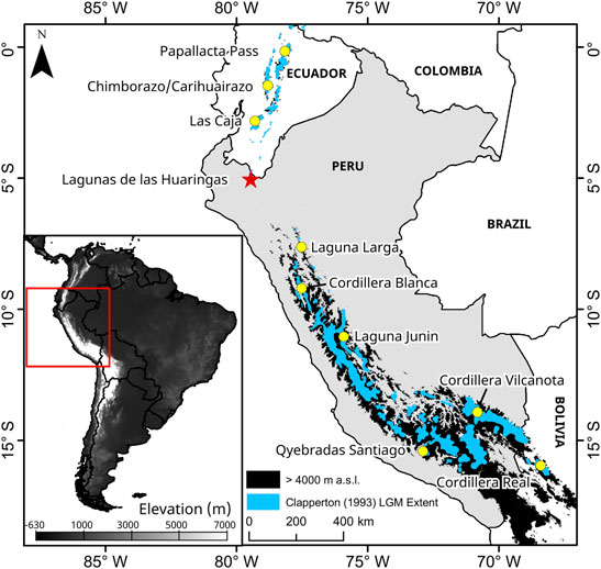
FIGURE 1. Map of Peru showing the study site location in northern Peru (red star; Lagunas de las Huaringas) within a data gap between former palaeoglaciological studies mentioned within the text (yellow circles). The majority of these locations are located above 4,000 m above sea level (a.s.l.) shown by the black outline. The hypothesised LGM extent is from Clapperton (1993) shown by the blue outline.

We aim to reconstruct the palaeoglacial dynamics of the Lagunas de las Huaringas, an area that had not previously received detailed investigation in the literature, except preliminary ice extent estimations from Clapperton (1993). We provide: 1) a detailed glacial geomorphological map of the region; 2) a reconstruction of the likely maximum glacial extent, along with a reconstructed equilibrium line altitude (ELA) for the reconstructed ice masses; and 3) ELA-derived palaeotemperature estimates for the Local Last Glacial Maximum (LLGM), used to discuss the palaeoclimate implications of our findings. These outputs aid in allowing us to determine if glacial ice was present at this location, to understand the glacial dynamics, to assess whether the region incurred valley glaciation or an icecap with outlet glaciers, and to determine the potential climate glaciers would have formed under.

2 Study Area

2.1 Lagunas de las Huaringas

Lagunas de las Huaringas (here after referred to as Las Huaringas; ∼3,900 m a.s.l.; 5°00′S, 79°27′W) is located in the northern highlands of Peru (Figure 1) within the Huancabamba river catchment (Lila et al., 2016). The underlying geology comprises Paleogene to Neogene age volcanic-sedimentary rocks (Gómez et al., 2019), and the region is not currently glaciated. The main valley, the Shimbe valley (Figure 2), stretches north to south for ∼22 km and is characterised by two major depressions; a smaller up valley section occupied by Laguna el Paramo and a larger section occupied by Laguna Shimbe, the latter having an estimated maximum water depth of ∼30 m. Within the Shimbe valley and throughout the study area, there are a number of smaller arcuate valleys with lakes dammed by ridges or bedrock indicative of past glaciation, the most striking of which are situated on the western side of the Las Huaringas Massif (Figure 2). An area that we assume to be Las Huaringas was suggested as likely to have been glaciated during the LGM by Clapperton (1993). Clapperton mapped areas of potential glacial ice cover within the tropical Andes based on his extensive field experience in the region, and an assumption that most topography above 3,400 m would have been covered by ice during the LGM (blue outlines in Figure 1). As far as we are aware, this mapping was not based on any specific fieldwork, especially within the Las Huaringas area, nor via the use of any remotely sensed analysis (e.g., satellite or aerial imagery). Las Huaringas was only one of several such locations where past glaciation was suggested as likely in the northern Peru and southern Ecuador region (Clapperton, 1993). Many of these potential formerly glaciated areas in the region surrounding Las Huaringas have, as far as can be found in the literature, received no investigation since. Analysis of modern-day satellite datasets, and reconnaissance fieldwork by the authors of this study, indicate that palaeoglacial landforms (e.g., moraines and eroded bedrock surfaces) are abundant and well preserved within Las Huaringas, supporting Clapperton’s hypothesis for glaciation at this locality.

FIGURE 2

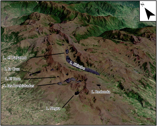
FIGURE 2. A Sentinel-2 optical imagery of Lagunas de las Huaringas (red star in Figure 1), draped over a 30 m ALOS DEM. This show the main central valley (Shimbe Valley) with the largest lake, Laguna Shimbe running almost along its entire length. Arcuate moraines and lake-filled depressions are seen on its western edge with their lake names detailed.

The climate of the Las Huaringas is subtropical and modulated by tropical Pacific Sea surface temperatures (SSTs) and ocean temperature at depths. These drive variations in the El Niño Southern Oscillation (ENSO) that itself influences interannual precipitation and air temperature variability (Garreaud, 2009; Kiefer and Karamperidou, 2019). Other influences include the transfer of moisture via the easterlies, which originate from the Atlantic Ocean, and track over the Amazon Basin incurring evapotranspiration. The easterlies flow over the eastern Andes brings enhanced precipitation, predominantly during the summer months, in response to the migration of the Inter-Tropical Convergence Zone (ITZC) southwards (Garreaud, 2009; Álvarez-Villa et al., 2011; Staal et al., 2018). On average, the Las Huaringas region receives ∼400 mm of precipitation per year, with the majority of precipitation falling between October and April (tropical summer season) with very little between June and August (tropical winter season). The intra-annual temperature variation of ∼0.5°C is exceeded by the diurnal temperature variation of ∼4°C.

2.2 Palaeoclimate of Northern Peru and Surrounding Areas During the LGM

Palaeotemperature and palaeoprecipitation can be reconstructed using a range of proxy records: palaeo-Equilibrium Line Altitudes (ELAs) from reconstructed glaciers (e.g., Porter, 2001), ice-cores (δ¹⁸O and ²H) (e.g., Thompson et al., 1998), lake sediment cores (e.g., pollen and diatoms) (e.g., Stansell et al., 2014), and palaeoecological techniques (e.g., Chevalier et al., 2020). Temperature reconstructions from palaeo-ELA reconstructions have estimated the LLGM temperature of Peru to range between 6.4 and 2°C cooler than present (Rodbell, 1992; Mark and Helmens, 2005; Ramage et al., 2005; Smith et al., 2005; Bromley et al., 2011a; Úbeda et al., 2018). The wide range in the estimated values is due to local controlling factors such as local topography, aspect, and relief. Some of the lowest estimates of temperature depression are yielded from glaciers constrained by topography sourced from predominantly westward facing cirques (−2.5°C; Ramage et al., 2005; −2 to −4°C; Smith et al., 2005), while higher estimates of cooling have been either from topographically unconstrained localities (e.g., volcanos) (−6.4°C; Úbeda et al., 2018) or glaciers that were predominantly eastward facing (−5 to −6°C; Rodbell, 1992). These suggest an east to west gradient yielding differing temperature reconstructions (Klein et al., 1999). δ¹⁸O analysis of ice-cores from the Sajama and Huascarán ice-caps suggests a potential LGM cooling of 8–12°C (Thompson et al., 1995; Thompson et al., 1998), consistent with a substantially cooler LGM climate. Sea surface temperatures also support a cooler LGM, with reconstructed tropical Pacific sea surface temperatures 2.8°C cooler than present (Lea et al., 2000), similar to the 2.3°C cooler global average (CLIMAP, 1976).

Palaeohydration studies from lake cores and other palaeoecological studies in the outer tropics demonstrate latitudinal and regional variability in precipitation patterns. Lake cores and palaeo-shorelines from more northern locations within the northern tropical Andes indicate a wetter LGM (Rodbell, 1993; Clapperton et al., 1997a; Chepstow-Lusty et al., 2005) linked to an intensified South American Summer Monsoon (SASM) in response to orbital variations (Baker et al., 2001). Other studies within the Bolivian Altiplano (straddling southern Peru and northern Bolivia) indicate little to no increase in precipitation during the LGM (Placzek et al., 2013; Nunnery et al., 2019), although there was an effective amount of moisture to maintain lake levels. Palaeoecological studies from the Amazon basin, an important location for moisture transfer to Peru and Bolivia, suggest it was drier during the LGM (Mourguiart and Ledru, 2003; Häggi et al., 2017; Novello et al., 2019). It has been hypothesised that increased LGM precipitation identified from lake sediment records in the Peruvian and northern Bolivian Andes was possible even with a drier Amazon basin (Vizy and Cook, 2007). This would be because zonal low-level flow would be able to move over the Andean mountains directly, convecting upwards rather than paralleling the Andes to the north (seen in the modern day), thereby creating an east-west precipitation gradient during the LGM.

3 Methods

3.1 Datasets

A geomorphological map and glacial reconstruction were based on analysis of multiple remotely sensed high-resolution images and digital elevation models (DEMs) (Supplementary Table 1). Newly-acquired high resolution tri-stereo SPOT 7 (1.5 m) and archived Pléiades (0.5 m) imagery was obtained through the European Space Agency (ESA) from Airbus Defence and Space and the National Centre for Space Studies (CNES). Large portions of Las Huaringas were cloud covered in the Pléiades imagery, leading to the eastern side of Las Huaringas and the Laguna Shimbe valley not being mapped at the highest resolution. As a result, these areas were mapped using the most recent cloud free image which could be obtained from Landsat 8 (30 m, pansharpened to 15 m), Sentinel-2A (10 m), RapidEye (5 m) or PlanetScope (4 m). Openly available imagery from Google Earth™ and Bing Maps, with a mixture of resolutions, were used to complement the other optical datasets.

DEMs used included: 1) the 30-m resolution Advanced Land Observing Satellite (ALOS) DEM from the Japan Aerospace Exploration Agency (JAXA; https://global.jaxa.jp). This DEM was generated from images acquired between 2006 and 2011 from the Panchromatic Remote-sensing Instrument for Stereo Mapping (PRISM) sensor onboard the ALOS (Tadono et al. (2014); 2) a new high-resolution DEM of the study area generated from the tri-stereo SPOT 7 imagery. The process for generation of this DEM, along with an evaluation of its uncertainty, is outlined below. The 30 m ALOS DEM was initially used for macro scale geomorphological mapping, with the higher resolution DEM needed to permit identification of smaller scale landforms (e.g., recessional moraines) (Pearce et al., 2014; Chandler et al., 2018) and to confirm the interpretation of any landforms identified and mapped using the lower-resolution datasets.

3.2 Digital Elevation Model Generation

Satellite Pour l’Observation de la Terre (SPOT) 7 tri-stereo imagery acquired on 11th May 2020 was used to create the high-resolution DEM (Figure 3). The SPOT 7 images were processed to the primary product level by Airbus Defence and Space. The three SPOT 7 images were used to generate point clouds within ERDAS Imagine 2018’s Photogrammetry Suite. Using the LAS Dataset to Raster tool in ArcGIS 10.6.1 the generated point cloud was processed into a DEM. To generate the DEM the rational polynomial coefficients (RPCs) provided with each image were used to provide georeferencing and satellite characteristics. The tri-stereo imagery was tied together using ∼100 tie-points, although those with the highest RMSE were removed to minimise the RMSE for the triangulation. This generated a RMSE of 0.07 pixels for the tied-together images. A point cloud with over 28.4 million points was generated, producing a DEM with a spatial resolution of ∼2.5 m.

FIGURE 3

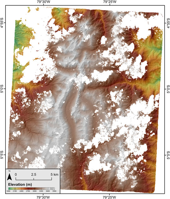
FIGURE 3. 2.5 m horizontal resolution SPOT 7 derived DEM of the Lagunas de las Huaringas area as a hillshaded image (azimuth: 315°, z-factor: 1) overlain by elevation. White “fuzzy” areas are no data generation errors removed due to cloud cover precluding data capture.

To interpolate across the point cloud and generate a DEM, Guo et al. (2010) suggests that the use of simple interpolation techniques (such as Natural Neighbor, Inverse Distance Weighting and Triangulated Irregular Network methods) are more efficient for high density data, such as that used within this study. To determine the best technique to interpolate between no data points within the DEM we compared “linear”, and “natural neighbour” approaches (“simple” interpolation was discounted as is can only interpolate over no data areas which are the size of a few pixels), that are present within the LAS Dataset to Raster tool. Using previously collected and processed dGPS points, acquired from the study area in 2017 as a control on absolute elevation, we determined the most accurate interpolation technique to be “Natural Neighbour”. Acquired dGPS points have a conservative estimate of uncertainty of ∼5 m due to the long baseline between rover and the local base station. The “Natural neighbour” method produced an elevation RMSE of 2.10 m compared to 2.14 m for the “linear” interpolation method, and there was no difference in the computational time between the two methods.

Large-scale landforms identified throughout the 30 m ALOS DEM and satellite imagery, demonstrated that the 2.5 m SPOT DEM was well aligned and thus the generated DEM required no further georeferencing. Many locations covered by the SPOT DEM were affected by cloud cover in the original imagery, while its resolution is not fine enough to allow adequate mapping of more subdued moraines (<2 m relief).

3.3 Geomorphological Mapping

Geomorphological mapping was conducted following well-established remotely sensed techniques (Chandler et al., 2018). We mapped geomorphological landforms determined to be of glacial origin using the criteria in Table 1, which follows a similar criteria to Glasser et al. (2008). Some landform criteria were not used due to landforms not being present or impossible to identify within our study region (e.g., shorelines). Small adjustments were made to the identification criteria for some features due to Glasser et al. (2008) mapping features in currently glaciated locations where landforms had a “fresher” appearance than those in our study area. Images were used in the “true colour” band combinations for their respective sensors, which allow a good assessment of landforms. To further enhance landform detection, where landforms were ambiguous by two-dimensional mapping, Google Earth™ was used for three-dimensional projection of remotely sensed imagery over topographic data, albeit sometimes at a lower resolution or lower quality imagery (Chandler et al., 2018). The mapping of glacial geomorphology includes moraines, trimlines, glacial lineations, cirques headwalls, glacial headwalls, boulders, and glacially smoothed bedrock. Non-glacial geomorphic features (e.g., streams and lakes) were also mapped to add context to the mapping. Due to datasets from multiple sensors being used to map features, and the errors and uncertainties associated with each of them, we conservatively estimate that mapped features might be horizontally offset from their true position by ±30 m (Supplementary Figure 1). Three of the authors visited the field area prior to this study, providing some limited ground truthing to mapped features within the Laguna Shimbe valley, though systematic and extensive fieldwork has not yet been undertaken.

TABLE 1

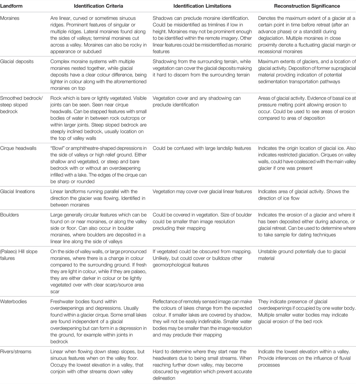
TABLE 1. Criteria for landform identification on remotely sensed imagery loosely modified from the landform identification criteria from Glasser et al. (2008).

3.4 Palaeoglaciological Reconstruction

We reconstructed the extent of all glaciers hypothesized to have occupied Las Huaringas to their most prominent and extensive mapped moraine. In the absence of any dating control on these moraines and any significant moraines between the cirque and these lower moraines, we assume that they represent the LLGM extents. This is consistent with the approach of other studies where dating controls are unavailable (e.g., Emmer et al., 2021). However, there is potential for some of the most downvalley glacial evidence in our study area to pre-date the LLGM. A number of studies have identified pre-LGM moraines down valley of glacial cirques within the northern tropical Andes (e.g., Goodman et al., 2001; Dirszowsky et al., 2005), although these would likely have much less relief and be less distinct compared to LLGM moraines. Without dating of moraines to create a chronology of glacial advances, it is currently not possible to constrain the age of the moraines at Las Huaringas.

We extracted basic metrics from these reconstructed glaciers, such as their mean, minimum and maximum elevations, glacier aspect and length. Where glaciers split into multiple outlets, we took the longest length. The cirque floor elevation was also extracted from the cirques from which glaciers were hypothesised to have originated from. Glacier ice surface contours were generated with contour intervals of 100 m to create ice surface profiles during their maximum extents. Contours were generated, in accordance with well established procedures detailed by earlier studies of glacier reconstructions (e.g., Sissons, 1974; Bendle and Glasser, 2012), across the glacier profiles. These contours were adjusted to be in-line with observed modern day glacial dynamics (Ng et al., 2010), with ice thickness reduced below the ELA (generation discussed below) closest to the terminus (convex contours), and with greater ice thickness above the ELA in areas closest to the headwall (concave contours).

The subjective nature of palaeo ice extent reconstruction is the main source of uncertainty for reconstructing palaeo glacier extent and thickness. Whilst lateral-terminal moraines provide elevation constraint and delimit potential glacier margins, they are not always present or easily identifiable. In such cases, a best estimate of the ice margin was determined using the elevation from the DEM using the terminus elevation of surrounding glaciers as a reference. The most common area where a best estimate was used was the terminus of the palaeo glaciers, where no well-defined (or mapped) terminal moraine could be delineated, or where lateral moraines are mapped on one side of the valley but were not apparent on the other. Uncertainty can also be seen in the glacier ice surface contours. Where ice split into two or more outlets from one accumulation source (e.g., Huancabamba 1), there may be some uncertainty as to how well they may represent the LGM ice surfaces. However, these were produced to provide a visual representation and were not used for any analysis.

3.5 Palaeo Equilibrium Line Altitude Reconstruction

The ELA is the theoretical line where accumulation and ablation are equal (Benn et al., 2005) and has been frequently used as a proxy of the surrounding climate conditions of temperature and precipitation for the reconstruction of tropical Andean glaciers and climate (Porter, 2001; Mark and Helmens, 2005; Bromley et al., 2011a; Martin et al., 2020). Although the ELA would not have been static for long periods of time due to the varying climate conditions, the reconstructed palaeo-ELA inferred in this study is assumed to be at its lowest potential elevation and thus represents the time the glaciers were at their most extensive (i.e., LLGM).

To reconstruct palaeo-ELAs we used the ArcGIS Toolbox created by Pellitero et al. (2015) which reconstructs palaeo-ELAs using a generated glacier DEM and using a number of different methods (MGE, AAR and AABR). We generated the glacier DEM using vertices of the glacier extent polygon to act as elevation and used the Natural neighbor interpolation method to reconstruct a flat glacier surface, as used in other studies for ELA reconstructions (e.g., Lee et al., 2021). This was then inputted into the Pellitero et al. (2015) tool using the Accumulation-Area Balance Ratio (AABR) method to generate the ELAs, as it has been shown to be the most accurate in reconstructing ELAs (Santos-González et al., 2013; Pearce et al., 2017; Quesada-Román et al., 2020). One of the main sources of uncertainty for the reconstruction of palaeo-ELAs using the AABR method is the choice of the balance ratio. There is however a lack of data on balance ratios across the tropical Andes, thus making the choice of balance ratio difficult to determine. Tropical glaciers generally have high ablation rates throughout the year, and also have small ablation areas (Rea, 2009). As such, some studies have assigned high balance ratios. For example, Quesada-Román et al. (2020) used a value of 2. To account for the uncertainty in constraining the balance ratio for tropical glaciers, several balance ratios were tested; 1.00, 1.25, 1.50, 1.75, 2.00, 2.25 and 2.50, with 1.75 being the global average (Rea, 2009). The use of multiple balance ratios results in variations in reconstructed ELAs by only a few tens of meters, or a ∼0.87% difference (if any difference is seen). The balance ratio of 1.75 was therefore used within this study as a median between the two extremes. It is acknowledged that the balance ratio could be higher, however.

3.6 Palaeotemperature Reconstruction

The reconstructed palaeo-ELAs and subsequent ELA change (ΔELA) were used to reconstruct palaeo-temperature. Given the uncertainty about past climate in the region, three potential atmospheric temperature lapse rates (ATLR) were used to calculate temperature change (ΔT): −5.5, −6.5 and −7.5°C/km (Quesada-Román et al., 2020). Although the ELA is controlled by a range of climate conditions including precipitation (e.g., Stansell et al., 2007), temperature has an overarching influence. The palaeo-ELA was compared to the modern ELA in order to calculate ΔELA. In this region the snowline lies above the highest local summit and therefore the nearest identifiable snowline that intercepted with topography was used to infer the modern ELA. The elevation of 4,600 m from a location ∼8°S was used (Hammond et al., 2018).

4 Results and Discussion

4.1 Geomorphological Interpretation and Reconstructed Glacier Extents

Within Section 4.1 we describe the results of both the geomorphological mapping (Figure 4) and reconstructed glacial ice extents (Figure 5) and metrics (Table 2). We provide a localised description and interpretation of our results for five geographical areas (Figure 5). These areas are: 1) Laguna Shimbe valley (LS); 2) eastern glacier valley (EG); 3) western glacier cirques (WG); 4) northern glacier valleys (NG); and 5) south-eastern glacier cirques (SEG). Reconstructed glacial ELAs and the estimated palaeotemperatures are reported study area wide and discussed.

FIGURE 4

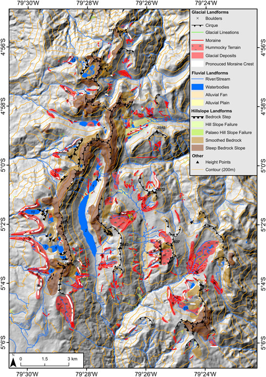
FIGURE 4. Geomorphological map of the Lagunas de las Huaringas. Basemap is a hillshade of the 30 m ALOS DEM (Azimuth: 315°, Z-factor: 1). A full resolution A0 version of the map can be found within the supplementary information. Lake names are: 1 – L. el Paramo; 2 – L. Shimbe; 3 – L. Redonda; 4 – L. Negra; 5 – L. las Arrebiatadas 1; 6 – L. las Arrebiatadas 2; 7 – L. las Arrebiatadas 3; 8 – L. las Arrebiatadas4; 9 – L. el Toro; 10 – L. la Cruz; 11 – L. el Rey Inca; 12 – L. Negra de San Pablo; and 13 – L. Redondo de Zapalche.

FIGURE 5

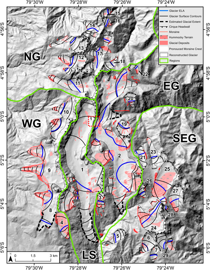
FIGURE 5. Reconstructed glacial extents within the Lagunas de las Huaringas along with reconstructed ELAs, glacier surface contours (100 m interval) and geomorphic evidence (i.e., moraines) used to delineate the glaciers. Glaciers 1, 2 and 8 have estimated glacier extents shown by the dashed lines. Extents overlie a hillshade of the 30 m ALOS DEM (azimuth: 315°, z-factor 1). The five areas defined for interpretations are delineated by thick green lines. These also define the extents in subsequent figures. Names and reconstructed ELA elevations of glaciers relate to those shown in Table 2 within the ELA reconstruction section. Acronyms are: LS–Laguna Shimbe valley (Figure 6); EG–Eastern Glacier valley (Figure 8); SEG–South-Eastern Glacial cirques (Figure 9); WG–Western Glacier cirques (Figure 10); and NG–Northern Glacier valleys (Figure 11). Subset 1 shown by the dashed lines corresponds to the col shown in detail within Figure 7.

TABLE 2

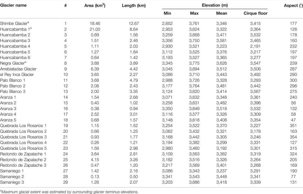
TABLE 2. Metrics of area, length, glacier elevation, aspect, cirque floor elevation for reconstructed glaciers. Glacier # corresponds to the numbers in Figure 5. Glacier names are derived from either a named lake that occupies a depression within the valley, the cirque the glacier occupied (e.g., Shimbe), or the nearest named river the valley flows into (e.g., Huancabamba). Aspect visualised in Supplementary Figure 2.

Across the study area we identified a number of moraines, while mapping over 830 moranic fragments or singular prominent moraine features, 44 individual glacial cirques with floor elevations ranging from between ∼3,150 and 3,600 m, 38 mapped glacial lineations with lengths between ∼23 and 103 m, 32 bedrock steps, a number of individual boulders mapped within or on a moraine that may be used for dating purposes, hill slope failures, smoothed bedrock surfaces, and hummocky terrain. All these features are used to evidence glacial activity and their extent within the Las Huaringas region.

4.1.1 Laguna Shimbe Valley

The mapped geomorphology (Figure 6A) suggests a large valley glacier formed in the central Laguna Shimbe valley (LS) during the LLGM (Figure 6B). This glacier (“Shimbe Glacier”) likely extended to a minimum elevation of 2,652 m, 12.7 km down valley, with a reconstructed area of 18.46 km². Lateral moraines are located along the western wall of the Shimbe valley, at ∼3,420 and ∼3,340 m, respectively, and constrain the lateral and vertical extent of the glacier. However, the greatest extent of the Shimbe Glacier cannot be established confidently due to downvalley evidence being difficult to discern. This may be due to postglacial erosion and fluvial reworking. As a result, we provide a hypothesised maximum LLGM limit for the Shimbe Glacier.

FIGURE 6

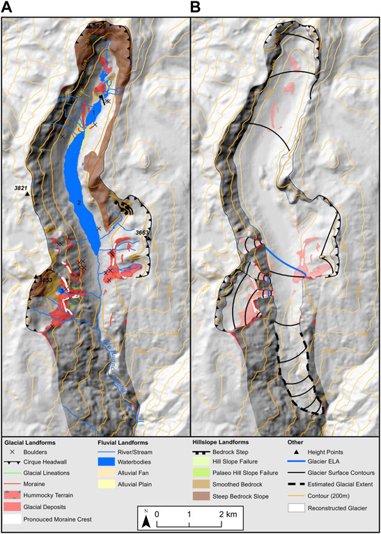
FIGURE 6. The Laguna Shimbe valley (LS) with (A) mapped glacial geomorphology, and (B) reconstructed glacier to its estimated LLGM extent. Base map is a hillshade of the 30 m ALOS DEM (azimuth: 315°, z-factor 1). Lake names: 1 – L. el Paramo, 2 – L. Shimbe.

Between the hypothesised maximum glacial extent, and moraines further up valley (∼9 km), little geomorphic evidence is apparent (Figure 6). This may be due to rapid retreat from its maximum extent during deglaciation, burial of evidence (e.g., by peat accumulation) or fluvial reworking of evidence. Some moraines are observed, though they are likely due to ice flow from glacial cirques on either side of the main valley. Closely spaced (∼20 m) moraines between Laguna el Paramo (lake #1) and the larger Laguna Shimbe (lake #2) (Figure 6) could indicate glacial advances that postdate the LLGM, either during the late-glacial or early-Holocene. Glacial advances of these ages have been documented in a number of studies in Peru (e.g., Bromley et al., 2011b) and northern Bolivia (e.g., Zech et al., 2007).

Glacial cirques are located along the LS valley walls with cirque floor elevations between ∼3,370 and 3,550 m a.s.l. (Figure 6). These cirques contain geomorphic evidence with moraines both within and just outside their cirque confines, indicating that during their maximum extent these would have coalesced with the main trunk of the Shimbe glacier. Closely spaced moraines just beyond, or within, the glacial cirques suggests that glaciers that occupied these cirques became decoupled from the Shimbe glacier during post-LLGM deglaciation and did not reconnect during any subsequent glacial advances. The geomorphic evidence suggests that the Shimbe glacier did not advance back to, or close to, its former extent after deglaciation from its LLGM maximum.

Near the head of the Shimbe Valley there is a topographic low (“col”) at ∼3,460 m a.s.l. on the eastern valley wall (Figure 7). This dip features smoothed bedrock, compared to the rougher surrounding valley walls, indicating it has been smoothed by glacial ice. Either a localised glacier was present at this location adjacent to the Shimbe glacier, or the Shimbe glacier was thick enough to overcome the valley topography and flow into the adjacent valley. To allow ice to overcome the col, it would have required a minimum ice thickness of ∼200 m thicker than any other LLGM reconstructed ice masses across the study area.

FIGURE 7

FIGURE 7. Confluence of glacier ice at the col with the location can be seen in Figure 5 1), that shows the connection (red circle) between the Shimbe glacier and Huancabamba 1 glacier during their LLGM maximum extent in a col with a maximum elevation of 3,464 m a.s.l. that is lower than the surrounding valley wall ridges (3,646 m a.s.l.). Yellow contours are at 100 m intervals.

4.1.2 Eastern Glacial Valley

The valley to the east of LS exhibits extensive evidence of glaciation with a number of mapped moraines along the valley walls and floor, eight distinct glacial cirques, and nineteen mapped glacial lineations (Figure 8A). The evidence suggests one of the largest glaciers within the Las Huaringas region, with a reconstructed estimate of the Huancabamba 1 glacier area of 21 km² (Figure 8B). The extents and area metrics of the reconstructed glacier are an estimate, due to the absence of any discernible cross valley terminal moraines downvalley. The geomorphic evidence within the EG suggests an interconnected glacial valley system with three terminus locations, that can be split into two distinct “zones”; 1) the valley running south paralleling the Shimbe valley with a singular glacier terminus, and 2) the two valleys, with a glacier terminus each, to the north which run eastward–all hypothesised to have terminated at ∼3,000 m a.s.l. due to the absence of obvious terminal moraines (Supplementary Figure 5). All valleys within the EG area contain valley wall cirques with cirque floor elevations ranging from 3,178–3,420 m a.s.l. At their largest extent, glaciers flowing from these cirques would have connected with the main valley glacier during the LLGM. Similar to the cirque glaciers reconstructed in the LS area, mapped moraines beyond and within their cirque extents suggests that after deglaciation from the LLGM any subsequent readvances would not have seen their reconnection with any main valley glacier, otherwise such evidence beyond their cirque confines would likely have been removed by glacial erosion.

FIGURE 8

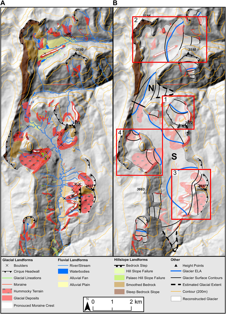
FIGURE 8. The Eastern Glacial valley (EG) with (A) mapped glacial geomorphology, and (B) the reconstructed glaciers to their estimated LLGM extent. The Huancabamba 1 glacier is split into two zones: the northern (N) and southern (S) zones. The separation is the split at the col that connected the two valleys, shown in Figure 7. Subsets (B) 1, 2, 3 and 4 correspond to Supplementary Figures 3, 4, 5 and 6, respectively. Base map is a hillshade of the 30 m ALOS DEM (azimuth: 315°, z-factor 1).

These two zones are split by the col (Figures 7, 8), through which the Shimbe and Huancabamba 1 glaciers could have potentially been connected at the height of their LLGM glacial extents. Evidence for this is smoothed bedrock exposed in the col between LS and EG suggesting that at some point the Shimbe glacier was thick enough (>200 m thickness) to overcome the topography and make a direct connection between these two glacial masses. Without further infield investigations however, we cannot determine whether this occurred at the LLGM or during an earlier glaciation.

Evidence for the potential “spill over” of ice from the LS to the EG area can be seen within the northern zone of EG (Figure 8 section labelled N). This zone has two eastward flowing valleys, with the most southerly valley exhibiting little evidence for glaciation apart from a singular glacial cirque on either side of the valley. The southernmost cirque (Figure 8B subset 1; Supplementary Figure 3) has a well-developed set of moraines perhaps indicating multiple glacial events. The northernmost valley hosts the most striking evidence with a prominent medial moraine (Figure 8B subset 2; Supplementary Figure 4) running down the centre of the valley going eastward. This demonstrates that glacial ice flowed both from the glacial cirques in the northern valley and from the south, potentially from ice flowing over from SG area. This southern input is hypothesised due to the absence of a clear glacial cirque above the valley. The medial moraine is located to the southern side of the east-west trending valley, suggesting that ice flow was dominated by flow originating from the northern cirques.

Within the southern zone of the EG area (Figure 8 section labelled “S”), are a number of predominantly westward facing glacial cirques, the majority of which exhibit classic evidence of cirque glaciation. These would have likely contained ice, feeding into the main Huancabamba glacier flowing southward, during their most extensive LLGM extent. Two cirques are of particular interest within the southern zone of the EG: 1) one near the southern end on the east side of the valley (Figure 8 subset 3; Supplementary Figure 5), and 2) the other on to western flanks (Figure 8 subset 4; Supplementary Figure 6). The first location contains three reconstructed glacier outlets connecting to an individual cirque. Prominent moraines connect through all three outlets and appear to have once contained lakes within each outlet depression. Moraines may delineate individual advances after the LLGM when they become disconnected from the main valley glacier during deglaciation. These lakes were moraine dammed and drained at some point after deglaciation. This was probably the result of moraine dam failures, evidenced by the lack of an enclosing terminal moraine and deposits of alluvial material in front of the glacial moraines. Within the second location, the glacial cirque splits into two outlets, with the southern outlet being one of only two locations that exhibit possible glacial lineations. There is a potential for these features to be glacial flutes, however because of their small-scale further investigation with a finer resolution DEM along with infield techniques is required.

4.1.3 South-Eastern Glacial Cirques

Geomorphological evidence within the south-eastern zone (SEG) of the study area (Figure 9A), suggests a cirque to valley glacier configuration (Figure 9B). There are twelve identified cirques that would likely have contained reconstructed glaciers in this zone. The reconstructed glacial area during the LLGM was 17.7 km². Multiple moraines are nested within many of the cirques, but glacial geomorphic evidence is more discontinuous further south. The absence of this evidence is likely due to decreasing topographic elevation, which may not have permitted glacier ice to persist even during the LLGM. Many cirques exhibit extensive erosion with glacially smoothed bedrock indicative of warm-based basal conditions, in line with evidence across the study region. Many of the cirques would have contained a separate and confined glacier, with no evidence for ice masses coalescing. The dominant orientation for cirques in this zone is south and south-westward facing, which could be due to the predominant direction of incoming solar radiation in the southern hemisphere.

FIGURE 9

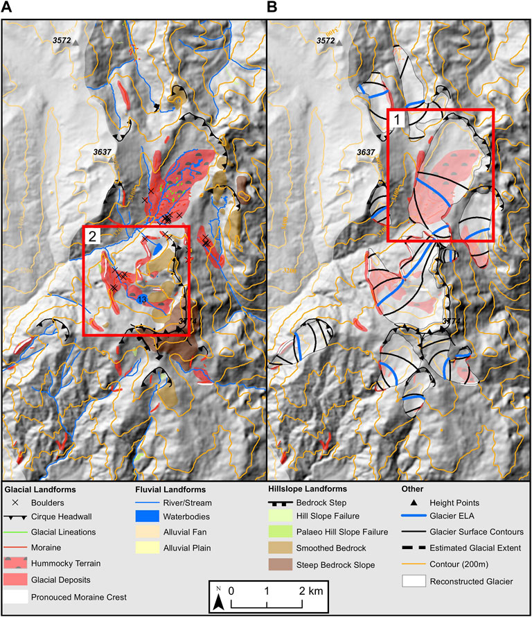
FIGURE 9. The southeastern glacial cirques (SEG) with (A) mapped glacial geomorphology, and (B) the reconstructed glaciers to their LLGM extents. Subsets (B) 1 and (A) 2 correspond to Supplementary Figure 7 and Supplementary Figure 8, respectively. Base map is a hillshade of the 30 m ALOS DEM (azimuth: 315°, z-factor 1). Lake name: 13 – L. Redondo de Zapalache.

Similar to the EG, the SEG zone is the only other location within the study area to contain mapped lineation features (Figure 9A subset 1; Supplementary Figure 7). nineteen features were mapped with lengths between 23 m and 100 m. These lineations are located within the extent of the Redondo de Zapalache 2 glacier valley (#25) behind discontinuous closely spaced moraines, with the orientation of the lineations indicating a northeast to southwest direction of glacier flow, similar to that suggested by the lineations in the EG valley. We hypothesise that these lineations are only found in these two locations due to their relatively unusual location on flat terrain. The remainder of the study area either lacks wide areas of sufficiently flat terrain where such lineations may develop, or lineations may have existed previously but have been eroded by post-depositional geomorphic action.

The Redondo de Zapalache 1 glacier area (#24) (Figure 9B subset 2; Supplementary Figure 8) is unique compared to the surrounding glacier cirques in the SEG zone, being similar to the two cirque glaciers discussed within the EG. The geomorphological evidence here suggests two glacier outlets that flowed from a shared accumulation zone. The total reconstructed glacier area was 3.6 km². Prominent moraines indicate maximum lateral extents of these ice masses. Further lateral moraines up-valley from these lateral-terminal moraines indicate that the two glacier outlets separated during deglaciation, dividing into two glaciers each occupying their own cirque, and potentially producing moraines suggesting post-LLGM readvance. The westernmost outlet of this glacier contains multiple closely spaced moraines (20–100 m apart) at its terminus potentially indicating a fluctuating ice front.

4.1.4 Western Glacial Cirques

The western zone of the Las Huaringas region (WG) contains some of the largest and most extensive moraines in the study region (Figure 10A). These moraines extend down to a minimum elevation of ∼3,100 m a.s.l. We reconstructed three glaciers, the Arrebiatadas Glacier, the el Rey Inca glacier and the Negra Glacier (Figure 10B), which occupy five large west-facing cirques. These cirques have steep headwalls and are well developed, indicating significant backward erosion while also having wide open backwalls that do not follow an amphitheatre-like shape that is seen across the study area; this makes it hard to determine an individual “source” cirque. Depressions containing water bodies are common across the WG. These twenty-six bodies of water are either dammed by bedrock (e.g., Lagunas las Arrebiatadas) or a moraine (e.g., Lagunas la Cruz), often coinciding with bedrock steps and smoothed bedrock indicating warmed based glaciers that produced significant glacial erosion with a high discharge of ice and a high mass turnover (MacGregor et al., 2000; Cook and Swift, 2012; Evans, 2021).

FIGURE 10

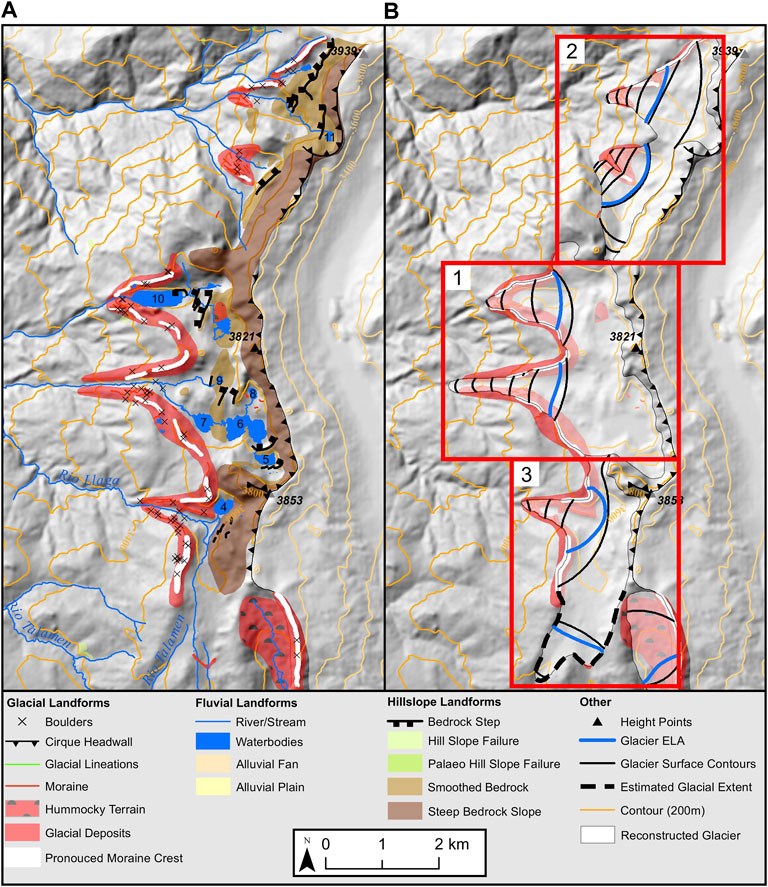
FIGURE 10. The western glacial cirques (WG) with (A) mapped glacial geomorphology, and (B) the reconstructed glaciers to their estimated LLGM extents. Subsets (B) 1, 2 and 3 correspond to Supplementary Figures 9, 10 and 11. Base map is a hillshade of the 30 m ALOS DEM (azimuth: 315°, z-factor 1). Lake names: 4 – L. Negra, 5 – L. las Arrebiatadas 1, 6 – L. las Arrebiatadas 2, 7 – L. las Arrebiatadas 3, 8 – L. las Arrebiatadas 4, 9 – L. el Toro, 10 – L. la Cruz, 11 – L. el Ray Inca.

The form of the Arrebiatadas Glacier (Figurer 10B subset 1; Supplementary Figure 9), and the el Ray Inca Glacier (Figure 10B subset 2; Supplementary Figure 10) suggest they both potentially had two source areas which coalesced to create an individual ice mass, from which two separate glacial outlets extended from. The Arrebiatadas Glacier area, covering 6.4 km², has well defined and interconnected moraines up-valley. These run down into, and demarcate, the individual outlets providing further evidence that ice came from a single source area. Moraines within the confines of the most extensive terminal moraine of the Arrebiatadas Glacier are closely spaced (20–50 m), which may indicate oscillating climate condition during formation. Similar dynamics are possible for the el Ray Inca Glacier. The el Ray Inca Glacier covered 3.6 km², had prominent lateral moraines on its northern most glacial outlet, and more closely spaced moraines near its terminus. Within the southern outline, it lacks many prominent moranic features, but hosts smaller closely-spaced moraines.

The Negra Glacier (Figure 10B subset 3; Supplementary Figure 11), the most southern of the glaciers in the WG area covered an area of 3.9 km². This glacier may have connected with the Arrebiatadas system at the LLGM as indicated by lateral moraines which appear to connect. Like other glaciers within WG, geomorphological evidence indicates that glacial ice flowed from a single source zone into two outlets, westward and southward. Although the moraines to the west clearly indicate the former glacier ice extent, little geomorphic evidence for the southern outlet is observed. Although a single moraine is mapped, no further evidence is seen to demark its most southerly advance, potentially indicating reworking from post-glacial fluvial action. Although glacial ice is reconstructed to the only mapped moraine in the outlet, due to the flatter profile of the topography when compared to its western counterparts, ice could have flowed further south than this position, but would require further infield investigation to determine this.

4.1.5 Northern Glacial Valleys

Glaciers reconstructed in the northern glacial valleys (NG) north study region generally exhibit a cirque- to valley-glacier configuration like the glaciers of the SEG area. Geomorphological evidence (Figure 11A) suggests the most extensive glaciers developed (Figure 11B) on the westward side of the region (mean ice mass area of 2.3 km²), while smaller glaciers developed to the east (mean ice mass area of 1 km²). These reconstructed glaciers cover a total area of 9.6 km² originating from twelve cirques with cirque floor elevations between 3,257 and 3,567 m a.s.l. One of the most striking features within this zone is the large bowl-like depression eroded down to bedrock with lakes filling the depression and bedrock joints (Figure 11 subset 1; Supplementary Figure 12). The significant erosion down to the bedrock, along with headward erosion of the cirque provides further evidence these glaciers had a high mass turnover during the LLGM.

FIGURE 11

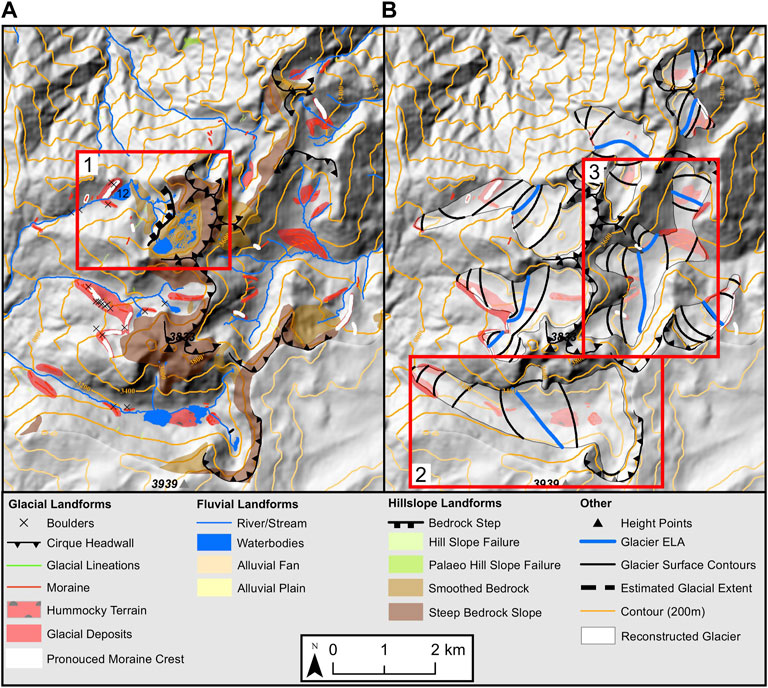
FIGURE 11. The northern glacial valleys (NG) with (A) mapped glacial geomorphology, and (B) the reconstructed glaciers to their estimated LLGM extents. Subsets (A) 1 and (B) 2 and 3, correspond to Supplementary Figures 12, 13 and 14, respectively. Base map is a hillshade of the 30 m ALOS DEM (azimuth: 315°, z-factor 1). Lake name: 12 – L. Negra de San Pablo.

Glaciers located on the western side of the NG zone have multiple moraines downvalley. These reach elevations as low as ∼3,100–3,200 m a.s.l. while each have multiple lakes either occupying a cirque depression or a depression behind a moraine dam further down valley (e.g., Laguna de San Pablo). This is in stark contrast to the eastern glaciers that have either no lake, or relatively small bodies of water. Glaciers in the northwest (Palo Blanco 1, 2 and 3) have reconstructed lengths of 4.79, 2.43, 2.00 km, respectively, with the longest seen in Figure 11 subset 2 (Supplementary Figure 13), the longest of any glaciers within the study area, but extend down to similar elevations to that of the Arrebiatadas and La Cruz glaciers. This could be due to the topography having a shallower incline (∼−11.4%) compared to those to the immediate west of the Shimbe valley (∼−18.5%), thereby allowing ice to flow further down valley while remaining at an elevation high enough to minimise mass loss.

Reconstructed glaciers located on the east side of the NG were generally limited to, or extended just beyond, their glacial cirques. The Aranza 4 glacier (Figure 11B subset 3; Supplementary Figure 14) is the only glacier to have evidence of any extensive advance, connecting with several cirque glaciers downvalley. Geomorphic evidence downvalley shows five lateral moraines towards it’s downvalley bend. These moraines are found at a range of elevations between 3,250 and 3,180 m, respectively. These could indicate a thinning glacier front during deglaciation from the LLGM. Glacier ice in the valley just above these lateral moraines (to its north) could have flowed down and connected with the main valley glacier during the LLGM (we have mapped this here), but it may have been limited to or just to the edge of the main valley glacier contributing little ice to the general flow of the main glacier.

4.2 ELA Reconstructions and Their Spatial Distribution

The reconstructed ELAs were derived from the reconstructed glacial ice extents using the AABR technique with a balance ratio of 1.75 ± 0.71 (Rea, 2009), ranged from 3,184 ± 27 m to 3,776 ± 33 m with a mean of 3,422 ± 30 m (Table 3). The reconstructed ELAs of glaciers without a confident determination of their terminal extent (e.g., Shimbe and Huancabamba 4 glaciers), may be lower or higher in elevation than that reported here. As expected, using higher and lower balance ratios give lower and higher ELAs, respectively. Rea (2009) and Quesada-Román et al. (2020) suggest a higher balance ratio may be more accurate for conditions within the tropical Andes. As shown by the comparison of lower and higher balance ratios, in this case, the balance ratios have little effect on the reconstructed ELA elevations with variations of up to only ∼20 m. This minimal difference does not affect temperature estimations significantly (∼± 0.2°C). We therefore recommend that similar studies should have confidence in using the global scenario (balance ratio of 1.75) for locations which do not have detailed studies on their accumulation-ablation balance ratios determined for ELA reconstructions. Although the global balance ratio produces little variance in results, the largest variance stems from accurate delineation of the past glacial extent. If ice limits are not accurate, they could have significant influence on local and regional climate interpretations.

TABLE 3

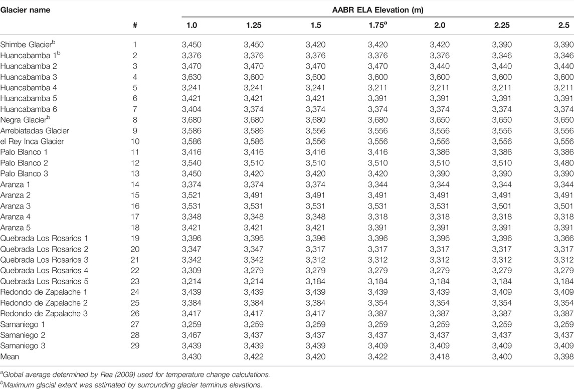
TABLE 3. Results of the palaeo-ELA calculations (m) using the AABR method with different ratios.

Within our ELA reconstruction estimates there is an east-to-west gradient in the spatial distribution within Las Huaringas (Figure 12A). On average, the ELAs from glaciers situated on the eastern side of the study region had a lower reconstructed ELA while glaciers to the west had a higher ELA. This may suggest that the glaciers on the east side of Las Huaringas received more precipitation than those on the west side during the LLGM, resulting in a lower ELA. Similar east-to-west gradients have been identified by Porter (2001) and Martini et al. (2017) in their ELA reconstruction studies across the tropical Andes and Cordillera Oriental. This gradient is similar to the present day subtropical climate patterns and the movement of moisture via the easterly trade winds and trans-Andean flow, from the Amazon basin to the eastern flanks of the Andean mountains (Espinoza et al., 2020). This brings an asymmetric precipitation pattern with increased rates in the east compared to the west (Kumar et al., 2019). A similar east-to-west gradient is seen for cirque floor elevations (Figure 12B). When compared with ELA elevations (Figure 12C) it could suggest that ELAs were lower in the east because the overall elevation is situated lower, but this could simply be because of increased maximum erosion at or below the ELA due to increased accumulation compared to the west, therefore lowering cirque floor elevations.

FIGURE 12

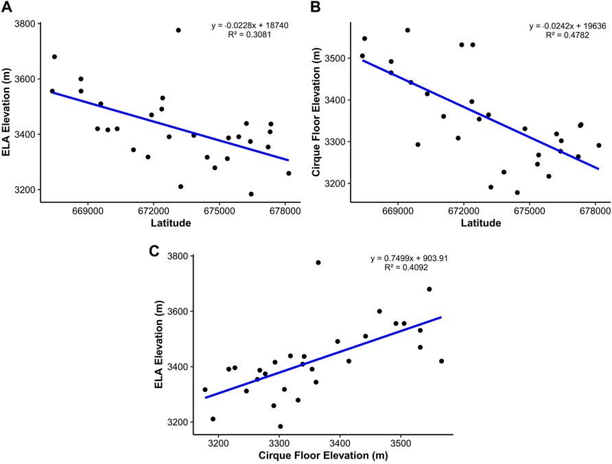
FIGURE 12. Elevations for (A) reconstructed glacier ELAs and (B) cirque floors against their locations latitudinally, and (C) the ELA elevation and cirque floor elevation plotted against each other.

4.3 Palaeotemperature Estimate and its Comparison to Surrounding Studies

The reconstructed LLGM ELAs for the Las Huaringas region were used to estimate palaeotemperature. It is simplistic to assume that temperature alone would have changed since the LGM to present, as precipitation would also have changed in response to temperature changes and atmospheric-circulatory system changes. Whilst we acknowledge the likely impact of precipitation changes on palaeo-glacier mass balance, being a key driver of tropical glaciations (Fyffe et al., 2021), a simple palaeotemperature reconstruction can aid in understanding the potential climate the glaciers would have been present under.

The mean ΔELA change across Las Huaringas, from LLGM to present is 1,178 ± 10 m. This represents an average ΔT of −7.6 ± 0.2°C using a ATLR of 6.5°C/km. Higher and lower ATLR predictably result in lower and higher average ΔT, with 6.5 and 8.9°C using ATLRs of 5.5 and 7.5°C/km, respectively.

Our lowest estimate of temperature cooling (i.e., 8.9°C) is consistent with other palaeo-ELA temperature reconstructions within the tropical Andes (see Supplementary Table 2) (Rodbell, 1992; Mark et al., 2005; Mark and Helmens, 2005; Ramage et al., 2005; Smith et al., 2005; Bromley et al., 2011a; Úbeda et al., 2018). Temperature cooling estimates from valley glaciation locations that are considerably lower than those reported by our study, with Ramage et al. (2005) reporting a cooling of 2.5°C in Lake Junin, and Smith et al. (2005) estimating a cooling between 2°C and 4°C for the Lake Junin and Milluni and Zongo valleys. This difference in results may be due to the higher elevation of those study areas, with the maximum elevation in Lake Junin and the Milluni and Zongo valleys being ∼4,600 m a.s.l. and ∼5,600 m a.s.l., respectively. This would require less cooling to initiate glaciation compared to lower elevation locations, such as ours. Thus, greater cooling would be needed, if it is assumed only temperature changed, for extensive glaciation within Las Huaringas, due to the massif being below 4,000 m in elevation. However, if precipitation and temperature changed in tandem, then a smaller temperature change may be required (e.g., if the rate of precipitation was higher during the LLGM).

There are very few studies that produce LLGM temperature estimates from low elevation locations, especially in or near our study area. This makes comparisons difficult, as study sites that are distant from Las Huaringas are likely to be affected by different climate influences. Our higher temperature cooling estimate is closer to estimates from the Merida Andes with a lowest estimated cooling of 6.4°C (Stansell et al., 2007), the High Plain of Bogotá with a cooling of 7.6°C (Mark and Helmens, 2005), and modelled temperature changes across the Bolivian and Peruvian Andes from the Junín Valley, Cordillera Vilcanota and Laguna Kollpa Kkota, where a cooling of 5–9°C has been reported (Klein et al., 1999). The two former studies, though higher in latitude (i.e., Venezuela and Colombia), did reconstruct similar temperature cooling from locations with a similar elevation (4,500 m a.s.l.) to Las Huaringas. Klein et al. (1999) estimates are from across the Bolivian and Peruvian Andes, but are from higher elevation locations above 5,000 m. Though this is significantly higher in elevation than our area, the temperature cooling estimates are similar. Estimates from other methods are also consistent with our results of a substantial cooling during the LLGM. Analysis of ice-cores from the Huascarán and Samaja ice-caps (Thompson et al., 1995; Thompson et al., 1998; Thompson et al., 2006), suggests potential cooling of between 5 and 8°C at the LLGM. Our two higher estimates from the ALTR (5.5 and 6.5°C/km) fall within their temperature range.

4.4 Uncertainties

The reconstructions presented here are based on their most extensively mapped moraine, which are assumed to be the LLGM extent of the reconstructed ice mass. However, these moraines could be later or earlier in age and that could affect the climate reconstruction derived from this study. The reconstructed glaciers have also been assumed to have advanced synchronously across the region. Whilst this would not impact maximum extent calculations (i.e., area and ELAs), without any dating of these features there are implications for LLGM timing and glacial-climate interactions. Because we are unable to attribute the advances and climate cooling to any specific time period or event we do not infer any regional or hemispheric scale palaeoclimatic significance from our analysis. We also inferred the glacier terminus position where no palaeoglacial evidence existed due to inferred postglacial processes, thus there will likely be uncertainties in glacier extent and ELA reconstructions. Without detailed fieldwork these uncertainties cannot be addressed.

Other uncertainties arise from the datasets used. Although the newly generated 2.5 m resolution DEM is the highest resolution DEM of the area available, clouds precluded mapping of certain areas of the region, whilst the general image quality limited its use for mapping small-scale geomorphic landforms or performing more detailed analysis. The collection of a cloud-free set of SPOT-7 images would allow more areas to be studied, whilst the generation of higher resolution DEMs (<10 m) or the collection of LiDAR data would allow finer resolutions DEMs (<1 m) with better data quality. If these data were generated, or openly released, for the tropical Andes, it would allow more detailed geomorphic mapping of hard to access locations and allow more efficient field sampling campaigns (e.g., for dating purposes).

Lastly, the geomorphic mapping shown within this study is not constrained by any substantive field ground truthing which is typically standard in geomorphological studies (Chandler et al., 2018). Due to this, we cannot extract finer details in the geomorphic record, nor make any major inferences in the connectivity of the features to one another. Instead, our approach has been to report our “discovery” of the palaeoglaciation of Las Huaringas, to define the macro-scale geomorphology, reconstruct the maximum extent and glacial dynamics of the study area and to showcase the substantial potential of the study area for further investigation.

4.5 Future Work

This study demonstrates that there is an abundance of geomorphic evidence for former glaciation within the Las Huaringas region. This confirms that the area was glaciated, which we hypothesise to have occurred at and since the LLGM (Clapperton, 1993). While this work does not quantitatively confirm the timing of glaciations, dating of glacial landforms would enable a more complete understanding of the timing and nature of the glaciation. Multiple moraines point to several periods of glacial advances, potentially Younger Dryas or later, with multiple moraine crests up-valley from the most extensive moraines identified and mapped here. Each of these systems could be specifically targeted for terrestrial cosmogenic nuclide dating, which would reveal the timing of glaciation. Lakes and peat-filled depressions exist within the limits of the glacial extent we reconstruct here, and these could be cored and dated to determine minimum and maximum limiting carbon dates of when they were uncovered (Lowe and Walker, 2014). This would fill a significant gap spatially between studies that date glacial advances in mid-Peru (Stansell et al., 2013), and those in more southerly Ecuador (Clapperton, 1990; Heine and Heine, 1996). It would also provide an understanding of glaciation in low elevation locations, which have not previously been studied, and independent assessment of any cosmogenic dating.

Limited numerical modelling has been conducted of tropical Andean valley glaciation, with the focus in South America primarily on the icefields of Patagonia (e.g., Hubbard et al., 2005; Collao-Barrios et al., 2018). Numerical modelling of the Las Huaringas valley system, and potentially other valley systems in the wider region, would enable a better understanding of the climatic requirements for glaciation in these low-elevation low-latitude locations. Detailed geomorphic mapping can be used to test and constrain any modelled ice extents. This is important within the Las Huaringas region as it is located in a transition zone between the inner and outer tropical climates, which are under different patterns of precipitation which enable glacial formation and development (Kaser, 2001). A potential understanding of the climate that permitted ice mass development, particularly during the LGM, can aid in furthering our overall comprehension of the LGM climate in the northern tropical Andes.

Clapperton (1993) inferred several areas that may have incurred LGM glaciation within the northern tropical Andes and beyond. Many of these have never been tested with detailed investigations such as those demonstrated by this study. There are still several locations (e.g., in southern Ecuador) that have yet to receive any study which confirms or refutes Clapperton’s inferred glaciation extent. With advancements in remote sensing technology, including access to high-resolution satellite imagery and the generation of high resolution DEMs (<30 m) being easily generated, or becoming more freely available, these locations can now be explored with relative ease. This would enable a better understanding of glacial dynamics within the tropical Andes, along with glacial-climatic interactions (e.g., testing hypotheses of east-west ELA and precipitation gradients). Further, with this plethora of high-resolution data, previously studied areas in Ecuador (e.g., Hastenrath, 1981) should warrant an updated investigation using new techniques and datasets to confirm their existence and the timing and glaciology of their glaciation.

5 Conclusion

The detailed mapping and glacial reconstruction presented here provides the first evidence for glaciation within the Las Huaringas region of northern Peru. It shows that extensive highly-erosive warm-based ice masses were present, likely at the LLGM. The dominant type of glaciation is valley type, with valley glaciers extending from cirques, with some potentially interconnected glacial systems over cols. The present evidence is not consistent with ice cap glaciation. This work supports the hypothesis of Clapperton (1993) that glacial ice was likely present at relatively low elevation sites in northern Peru during the LGM.

The geomorphic mapping was used to reconstruct glacier extents and to calculate palaeo-ELA estimates. Palaeotemperatures of between 6.5°C and 8.8°C cooler than present were determined. These are within the upper limits of other valley palaeoglaciological reconstruction based palaeotemperature estimates. Evidence for an ELA asymmetry of east-to-west (lowest to east, highest in the west), is in agreement with the present-day flow of moisture and climate patterns, suggesting that the broader climate circulatory systems in the region may not have been very different at the LLGM.

The exact timing of this glaciation is unknown. The absence of dated moraines means that best estimates for the age of glaciation are determined by assuming an LLGM-age for the most extensive sets of mapped moraines. Within Las Huaringas, moraines behind the most extensive extents mapped are hypothesized to be younger than the LLGM and are likely late-glacial or early-Holocene in nature. Testing of these hypotheses would require further investigation using terrestrial cosmogenic nuclide dating, analysis and dating of sediment and peat cores, in conjunction with field and remote mapping.

The evidence found within the Las Huaringas region strongly suggests that other relatively low elevation areas of northern Peru, and the surrounding areas of the tropical Andes, were potentially glaciated during the LGM and warrant further investigation.

Data Availability Statement

The datasets presented in this study can be found in online repositories. The names of the repository/repositories and accession number(s) can be found in the article/Supplementary Material.

Author Contributions

EL designed the study and led the work; NR, AH, AR, SJ and DF provided guidance on the conceptualisation, research analysis and content, manuscript structure and suggested figures. AH, AR and NR conducted field reconnaissance of the study area prior to this research. EL conducted the data collection and analysis, led the writing of the manuscript and creation of the figures. NR, AH, AR, SJ and DF contributed to the interpretation and discussion of the results and aided in reviewing and editing the manuscript.

Funding

This study was supported and funded by the IAPETUS2, Natural Environment Research Council (NERC) Doctoral Training Partnership (DTP) grant NE/S007431/1, a NERC Urgency Grant (NE/R004528/1 to ACGH and NR) and a Royal Society Research Grant (RG120575 to ACGH). The Pléiades high resolution imagery and SPOT 7 tri-stereo satellite imagery were provided by CNES and Airbus DS, respectively, through ESA’s “data available for research and application development” project ID: 59560.

Conflict of Interest

The authors declare that the research was conducted in the absence of any commercial or financial relationships that could be construed as a potential conflict of interest.

Publisher’s Note

All claims expressed in this article are solely those of the authors and do not necessarily represent those of their affiliated organizations, or those of the publisher, the editors and the reviewers. Any product that may be evaluated in this article, or claim that may be made by its manufacturer, is not guaranteed or endorsed by the publisher.

Acknowledgments

The Pléiades imagery (© CNES 2020) and SPOT 7 (© Airbus DS 2020), stereo satellite images were provided through ESA by CNES and Airbus DS. Landsat and Sentinel-2 satellite images were provided by USGS and ESA, respectively, and the ALOS DEM was provided by the JAXA. We would like to thank Rodolfo Rodriguez of the Universidad de Piura for the modern climate data and support with field logistics during the initial preliminary field work. We would also like to thank Rachel Carr and Stuart Dunning from Newcastle University, Arminel Lovell from the Carbon Disclosure Project (CDP), and Liam Taylor from the University of Leeds for aiding in the generation of the SPOT 7 DEM. All mapping of geomorphology was conducted in QGIS, while figure making was conducted in ArcMap 10.8.1.

Supplementary Material

The Supplementary Material for this article can be found online at: https://www.frontiersin.org/articles/10.3389/feart.2022.838826/full#supplementary-material

References

Álvarez-Villa, O. D., Vélez, J. I., and Poveda, G. (2011). Improved Long-Term Mean Annual Rainfall fields for Colombia. Int. J. Climatol. 31 (14), 2194–2212. doi:10.1002/joc.2232

CrossRef Full Text | Google Scholar

Angel, I., Guzman, O., and Carcaillet, J. (2017). Pleistocene Glaciations in the Northern Tropical Andes, South America (Venezuela, Colombia and Ecuador). Cuadernos de Investigacion Geografica 43 (2), 571. doi:10.18172/cig.3202

CrossRef Full Text | Google Scholar

Angel, I. (2016). Late Pleistocene Deglaciation Histories in the central Mérida Andes (Venezuela). Ph. D. Grenoble, France: Université de Grenoble Alpes-Universidad Central de Venezuela.

Google Scholar

Baker, P. A., Rigsby, C. A., Seltzer, G. O., Fritz, S. C., Lowenstein, T. K., Bacher, N. P., et al. (2001). Tropical Climate Changes at Millennial and Orbital Timescales on the Bolivian Altiplano. Nature 409 (6821), 698–701. doi:10.1038/35055524

PubMed Abstract | CrossRef Full Text | Google Scholar

Bendle, J. M., and Glasser, N. F. (2012). Palaeoclimatic Reconstruction from Lateglacial (Younger Dryas Chronozone) Cirque Glaciers in Snowdonia, North Wales. Proc. Geologists' Assoc. 123 (1), 130–145. doi:10.1016/j.pgeola.2011.09.006

CrossRef Full Text | Google Scholar

Benn, D. I., Owen, L. A., Osmaston, H. A., Seltzer, G. O., Porter, S. C., and Mark, B. (2005). Reconstruction of Equilibrium-Line Altitudes for Tropical and Sub-tropical Glaciers. Quat. Int. 138-139, 8–21. doi:10.1016/j.quaint.2005.02.003

CrossRef Full Text | Google Scholar

Blard, P.-H., Lave, J., Farley, K. A., Ramirez, V., Jimenez, N., Martin, L. C. P., et al. (2014). Progressive Glacial Retreat in the Southern Altiplano (Uturuncu Volcano, 22°S) between 65 and 14 Ka Constrained by Cosmogenic 3He Dating. Quat. Res. 82 (1), 209–221. doi:10.1016/j.yqres.2014.02.002

CrossRef Full Text | Google Scholar

Bromley, G. R. M., Hall, B. L., Rademaker, K. M., Todd, C. E., and Racovteanu, A. E. (2011a). Late Pleistocene Snowline Fluctuations at Nevado Coropuna (15°S), Southern Peruvian Andes. J. Quat. Sci. 26 (3), 305–317. doi:10.1002/jqs.1455

CrossRef Full Text | Google Scholar

Bromley, G. R. M., Hall, B. L., Schaefer, J. M., Winckler, G., Todd, C. E., and Rademaker, K. M. (2011b). Glacier Fluctuations in the Southern Peruvian Andes during the Late-Glacial Period, Constrained with Cosmogenic 3 He. J. Quat. Sci. 26 (1), 37–43. doi:10.1002/jqs.1424

CrossRef Full Text | Google Scholar

Bromley, G. R. M., Schaefer, J. M., Hall, B. L., Rademaker, K. M., Putnam, A. E., Todd, C. E., et al. (2016). A Cosmogenic 10Be Chronology for the Local Last Glacial Maximum and Termination in the Cordillera Oriental, Southern Peruvian Andes: Implications for the Tropical Role in Global Climate. Quat. Sci. Rev. 148, 54–67. doi:10.1016/J.QUASCIREV.2016.07.010

CrossRef Full Text | Google Scholar

Bromley, G. R. M., Schaefer, J. M., Winckler, G., Hall, B. L., Todd, C. E., and Rademaker, K. M. (2009). Relative Timing of Last Glacial Maximum and Late-Glacial Events in the central Tropical Andes. Quat. Sci. Rev. 28 (23), 2514–2526. doi:10.1016/j.quascirev.2009.05.012

CrossRef Full Text | Google Scholar

Carcaillet, J., Angel, I., Carrillo, E., Audemard, F. A., and Beck, C. (2013). Timing of the Last Deglaciation in the Sierra Nevada of the Mérida Andes, Venezuela. Quat. Res. 80 (3), 482–494. doi:10.1016/j.yqres.2013.08.001

CrossRef Full Text | Google Scholar

Chandler, B. M. P., Lovell, H., Boston, C. M., Lukas, S., Barr, I. D., Benediktsson, Í. Ö., et al. (2018). Glacial Geomorphological Mapping: A Review of Approaches and Frameworks for Best Practice. Earth-Science Rev. 185, 806–846. doi:10.1016/j.earscirev.2018.07.015

CrossRef Full Text | Google Scholar

Chepstow-Lusty, A., Bush, M. B., Frogley, M. R., Baker, P. A., Fritz, S. C., and Aronson, J. (2005). Vegetation and Climate Change on the Bolivian Altiplano between 108,000 and 18,000 Yr Ago. Quat. Res. 63 (1), 90–98. doi:10.1016/j.yqres.2004.09.008

CrossRef Full Text | Google Scholar

Chevalier, M., Davis, B. A. S., Heiri, O., Seppä, H., Chase, B. M., Gajewski, K., et al. (2020). Pollen-based Climate Reconstruction Techniques for Late Quaternary Studies. Earth-Science Rev. 210, 103384. doi:10.1016/j.earscirev.2020.103384

CrossRef Full Text | Google Scholar

Clapperton, C. M., Clayton, J. D., Benn, D. I., Marden, C. J., and Argollo, J. (1997a). Late Quaternary Glacier Advances and Palaeolake Highstands in the Bolivian Altiplano. Quat. Int. 38-39, 49–59. doi:10.1016/s1040-6182(96)00020-1

CrossRef Full Text | Google Scholar

Clapperton, C. M., Hall, M., Mothes, P., Hole, M. J., Still, J. W., Helmens, K. F., et al. (1997b). A Younger Dryas Icecap in the Equatorial Andes. Quat. Res. 47 (1), 13–28. doi:10.1006/QRES.1996.1861

CrossRef Full Text | Google Scholar

Clapperton, C. M. (1990). Glacial and Volcanic Geomorphology of the Chimborazo-Carihuairazo Massif, Ecuadorian Andes. Trans. R. Soc. Edinb. Earth Sci. 81 (2), 91–116. doi:10.1017/S0263593300005174

CrossRef Full Text | Google Scholar

Clapperton, C. M. (1993). “Late Cenozic Glacial History of the Andes Part III: The Last Glacial Maximum (Isotope Stage 2),” in Quaternary Geology and Geomorphology of South America (Oxford, UK: Elsevier), 395–424.

Google Scholar

CLIMAP (1976). The Surface of the Ice-Age Earth. Science 191 (4232), 1131–1137. doi:10.1126/science.191.4232.1131

PubMed Abstract | CrossRef Full Text | Google Scholar

Collao-Barrios, G., Gillet-Chaulet, F., Favier, V., Casassa, G., Berthier, E., Dussaillant, I., et al. (2018). Ice Flow Modelling to Constrain the Surface Mass Balance and Ice Discharge of San Rafael Glacier, Northern Patagonia Icefield. J. Glaciol. 64 (246), 568–582. doi:10.1017/jog.2018.46

CrossRef Full Text | Google Scholar

Cook, S. J., and Swift, D. A. (2012). Subglacial Basins: Their Origin and Importance in Glacial Systems and Landscapes. Earth-Science Rev. 115 (4), 332–372. doi:10.1016/j.earscirev.2012.09.009

CrossRef Full Text | Google Scholar

Dirszowsky, R. W., Mahaney, W. C., Hodder, K. R., Milner, M. W., Kalm, V., Bezada, M., et al. (2005). Lithostratigraphy of the Mérida (Wisconsinan) Glaciation and Pedregal Interstade, Mérida Andes, Northwestern Venezuela. J. South Am. Earth Sci. 19 (4), 525–536. doi:10.1016/j.jsames.2005.07.001

CrossRef Full Text | Google Scholar

Emmer, A., Le Roy, M., Sattar, A., Veettil, B. K., Alcalá-Reygosa, J., Campos, N., et al. (2021). Glacier Retreat and Associated Processes since the Last Glacial Maximum in the Lejiamayu valley, Peruvian Andes. J. South Am. Earth Sci. 109, 103254. doi:10.1016/j.jsames.2021.103254

CrossRef Full Text | Google Scholar

Espinoza, J. C., Garreaud, R., Poveda, G., Arias, P. A., Molina-Carpio, J., Masiokas, M., et al. (2020). Hydroclimate of the Andes Part I: Main Climatic Features. Front. Earth Sci. 8, 64. doi:10.3389/feart.2020.00064

CrossRef Full Text | Google Scholar

Evans, D. (2003). Glacial Landsystems. London: Routledge.

Google Scholar

Evans, I. S. (2021). Glaciers, Rock Avalanches and the 'buzzsaw' in Cirque Development: Why Mountain Cirques Are of Mainly Glacial Origin. Earth Surf. Process. Landforms 46 (1), 24–46. doi:10.1002/esp.4810

CrossRef Full Text | Google Scholar

Farber, D. L., Hancock, G. S., Finkel, R. C., and Rodbell, D. T. (2005). The Age and Extent of Tropical alpine Glaciation in the Cordillera Blanca, Peru. J. Quat. Sci. 20 (7-8), 759–776. doi:10.1002/jqs.994

CrossRef Full Text | Google Scholar

Fyffe, C. L., Potter, E., Fugger, S., Orr, A., Fatichi, S., Loarte, E., et al. (2021). The Energy and Mass Balance of Peruvian Glaciers. JGR Atmospheres 126 (23), e2021JD034911. doi:10.1029/2021JD034911

CrossRef Full Text | Google Scholar

Garreaud, R. D. (2009). The Andes Climate and Weather. Adv. Geosci. 22, 3–11. doi:10.5194/adgeo-22-3-2009

CrossRef Full Text | Google Scholar

Glasser, N. F., Clemmens, S., Schnabel, C., Fenton, C. R., and McHargue, L. (2009). Tropical Glacier Fluctuations in the Cordillera Blanca, Peru between 12.5 and 7.6ka from Cosmogenic 10Be Dating. Quat. Sci. Rev. 28 (27), 3448–3458. doi:10.1016/j.quascirev.2009.10.006

CrossRef Full Text | Google Scholar

Glasser, N. F., Jansson, K. N., Harrison, S., and Kleman, J. (2008). The Glacial Geomorphology and Pleistocene History of South America between 38°S and 56°S. Quat. Sci. Rev. 27 (3-4), 365–390. doi:10.1016/j.quascirev.2007.11.011

CrossRef Full Text | Google Scholar

Gómez, J., Schobbenhaus, C., and Montes, N. E. (2019). Geological Map of South America 2019, Scale 1:5,000,000. Paris: (Commission for the Geological Map of the World (CGMW), Colombian Geological Survey, and Geological Survey of Brazil). https://doi.org/10.32685/10.143.2019.929

Google Scholar

Goodman, A. Y., Rodbell, D. T., Seltzer, G. O., and Mark, B. G. (2001). Subdivision of Glacial Deposits in Southeastern Peru Based on Pedogenic Development and Radiometric Ages. Quat. Res. 56 (1), 31–50. doi:10.1006/qres.2001.2221

CrossRef Full Text | Google Scholar

Guo, Q., Li, W., Yu, H., and Alvarez, O. (2010). Effects of Topographic Variability and Lidar Sampling Density on Several DEM Interpolation Methods. Photogramm Eng. Remote Sensing 76, 701–712. doi:10.14358/PERS.76.6.701

CrossRef Full Text | Google Scholar

Häggi, C., Chiessi, C. M., Merkel, U., Mulitza, S., Prange, M., Schulz, M., et al. (2017). Response of the Amazon Rainforest to Late Pleistocene Climate Variability. Earth Planet. Sci. Lett. 479, 50–59. doi:10.1016/j.epsl.2017.09.013

CrossRef Full Text | Google Scholar

Hammond, J. C., Saavedra, F. A., and Kampf, S. K. (2018). Global Snow Zone Maps and Trends in Snow Persistence 2001-2016. Int. J. Climatol 38 (12), 4369–4383. doi:10.1002/joc.5674

CrossRef Full Text | Google Scholar

Hastenrath, S. (1981). The Glaciation of the Ecuadorian Andes. Rotterdam: Balkema Publishers.

Google Scholar

Hastenrath, S. (2009). Past Glaciation in the Tropics. Quat. Sci. Rev. 28, 790–798. doi:10.1016/j.quascirev.2008.12.004

CrossRef Full Text | Google Scholar

Heine, K., and Heine, J. T. (1996). Late Glacial Climatic Fluctuations in Ecuador: Glacier Retreat during Younger Dryas Time. Arctic Alpine Res. 28 (4), 496–501. doi:10.2307/1551860

CrossRef Full Text | Google Scholar

Helmens, K. F. (2004). “The Quaternary Glacial Record of the Colombian Andes,” in Developments in Quaternary Sciences. Editors J. Ehlers, and P. L. Gibbard (Elsevier), 115–134. doi:10.1016/s1571-0866(04)80117-9

CrossRef Full Text | Google Scholar

Hubbard, A., Hein, A. S., Kaplan, M. R., Hulton, N. R. j., and Glasser, N. (2005). A Modelling Reconstruction of the Last Glacial Maximum Ice Sheet and its Deglaciation in the Vicinity of the Northern Patagonian Icefield, South America. Geografiska Annaler: Ser. A, Phys. Geogr. 87 (2), 375–391. doi:10.1111/j.0435-3676.2005.00264.x

CrossRef Full Text | Google Scholar

Jomelli, V., Grancher, D., Brunstein, D., and Solomina, O. (2008). Recalibration of the Yellow Rhizocarpon Growth Curve in the Cordillera Blanca (Peru) and Implications for LIA Chronology. Geomorphology 93 (3-4), 201–212. doi:10.1016/j.geomorph.2007.02.021

CrossRef Full Text | Google Scholar

Kaser, G. (2001). Glacier-climate Interaction at Low Latitudes. J. Glaciol. 47 (157), 195–204. doi:10.3189/172756501781832296

CrossRef Full Text | Google Scholar

Kiefer, J., and Karamperidou, C. (2019). High‐Resolution Modeling of ENSO‐Induced Precipitation in the Tropical Andes: Implications for Proxy Interpretation. Paleoceanography and Paleoclimatology 34 (2), 217–236. doi:10.1029/2018pa003423

CrossRef Full Text | Google Scholar

Klein, A. G., Seltzer, G. O., and Isacks, B. L. (1999). Modern and Last Local Glacial Maximum Snowlines in the Central Andes of Peru, Bolivia, and Northern Chile. Quat. Sci. Rev. 18 (1), 63–84. doi:10.1016/S0277-3791(98)00095-X

CrossRef Full Text | Google Scholar

Kumar, S., Vidal, Y.-S., Moya-Álvarez, A. S., and Martínez-Castro, D. (2019). Effect of the Surface Wind Flow and Topography on Precipitating Cloud Systems over the Andes and Associated Amazon basin: GPM Observations. Atmos. Res. 225, 193–208. doi:10.1016/j.atmosres.2019.03.027

CrossRef Full Text | Google Scholar

Lea, D. W., Pak, D. K., Peterson, L. C., and Hughen, K. A. (2003). Synchroneity of Tropical and High-Latitude Atlantic Temperatures over the Last Glacial Termination. Science 301 (5638), 1361–1364. doi:10.1126/science.1088470

PubMed Abstract | CrossRef Full Text | Google Scholar

Lea, D. W., Pak, D. K., and Spero, H. J. (2000). Climate Impact of Late Quaternary Equatorial Pacific Sea Surface Temperature Variations. Science 289 (5485), 1719–1724. doi:10.1126/science.289.5485.1719

PubMed Abstract | CrossRef Full Text | Google Scholar

Lee, E., Carrivick, J. L., Quincey, D. J., Cook, S. J., James, W. H. M., and Brown, L. E. (2021). Accelerated Mass Loss of Himalayan Glaciers since the Little Ice Age. Sci. Rep. 11 (1), 24284. doi:10.1038/s41598-021-03805-8

PubMed Abstract | CrossRef Full Text | Google Scholar

Lila, F. D. H. P., Joshua, T. M. G. V., Solorzano, A. C. C., and Mott, G. M. G. C. (2016). Paisaje Cultural "Complejo de Lagunas las Huaringas. Editor M. D. Cultura. First ed. (Peru: Ministro de Cultura).

Google Scholar

Lowe, J. J., and Walker, M. (2014). Reconstructing Quaternary Environments. New York, USA: Routledge.

Google Scholar

MacGregor, K. R., Anderson, R. S., Anderson, S. P., and Waddington, E. D. (2000). Numerical Simulations of Glacial-valley Longitudinal Profile Evolution. Geology 28 (11), 1031–1034. doi:10.1130/0091-7613(2000)028<1031:nsogvl>2.3.co;2

CrossRef Full Text | Google Scholar

Mahaney, W. C., Kalm, V., Menzies, J., Hancock, R. G. V., and Milner, M. W. (2010). Reconstruction of the Pre-merida Glaciation, Northwestern Venezuelan Andes. Sediment. Geology. 230 (1), 10–20. doi:10.1016/j.sedgeo.2010.06.016

CrossRef Full Text | Google Scholar

Małecki, J., Lovell, H., Ewertowski, W., Górski, Ł., Kurczaba, T., Latos, B., et al. (2018). The Glacial Landsystem of a Tropical Glacier: Charquini Sur, Bolivian Andes. Earth Surf. Process. Landforms 43 (12), 2584–2602. doi:10.1002/esp.4417

CrossRef Full Text | Google Scholar

Mark, B. G., Harrison, S. P., Spessa, A., New, M., Evans, D. J. A., and Helmens, K. F. (2005). Tropical Snowline Changes at the Last Glacial Maximum: A Global Assessment. Quat. Int. 138-139, 168–201. doi:10.1016/j.quaint.2005.02.012

CrossRef Full Text | Google Scholar

Mark, B. G., and Helmens, K. F. (2005). Reconstruction of Glacier Equilibrium-Line Altitudes for the Last Glacial Maximum on the High Plain of Bogotá, Eastern Cordillera, Colombia: Climatic and Topographic Implications. J. Quat. Sci. 20 (7‐8), 789–800. doi:10.1002/jqs.974

CrossRef Full Text | Google Scholar

Mark, B. G., Rodbell, D. T., Seltzer, G. O., Goodman, A. Y., Castiglia, P. J., Moy, C. M., et al. (1999). “Late-Glacial Fluctuations of Ice Volume Inferred from Lakesediment Mineralogy and Terrain Modeling in the Cordillera Blanca, Peru,” in Spring AGU Conference. Boston, MA.

Google Scholar

Mark, B., Stansell, N., and Zeballos, G. (2017). The Last Deglaciation of Peru and Bolivia. Cig 43 (2), 591–628. doi:10.18172/cig.3265

CrossRef Full Text | Google Scholar

Martin, L. C. P., Blard, P.-H., Lavé, J., Jomelli, V., Charreau, J., Condom, T., et al. (2020). Antarctic-like Temperature Variations in the Tropical Andes Recorded by Glaciers and Lakes during the Last Deglaciation. Quat. Sci. Rev. 247, 106542. doi:10.1016/j.quascirev.2020.106542

CrossRef Full Text | Google Scholar

Martini, M. A., Kaplan, M. R., Strelin, J. A., Astini, R. A., Schaefer, J. M., Caffee, M. W., et al. (2017). Late Pleistocene Glacial Fluctuations in Cordillera Oriental, Subtropical Andes. Quat. Sci. Rev. 171, 245–259. doi:10.1016/j.quascirev.2017.06.033

CrossRef Full Text | Google Scholar

Mourguiart, P., and Ledru, M.-P. (2003). Last Glacial Maximum in an Andean Cloud forest Environment (Eastern Cordillera, Bolivia). Geol 31 (3), 195–198. doi:10.1130/0091-7613(2003)031<0195:lgmiaa>2.0.co;2

CrossRef Full Text | Google Scholar

Ng, F. S. L., Barr, I. D., and Clark, C. D. (2010). Using the Surface Profiles of Modern Ice Masses to Inform Palaeo-Glacier Reconstructions. Quat. Sci. Rev. 29 (23), 3240–3255. doi:10.1016/j.quascirev.2010.06.045

CrossRef Full Text | Google Scholar

Novello, V. F., Cruz, F. W., McGlue, M. M., Wong, C. I., Ward, B. M., Vuille, M., et al. (2019). Vegetation and Environmental Changes in Tropical South America from the Last Glacial to the Holocene Documented by Multiple Cave Sediment Proxies. Earth Planet. Sci. Lett. 524, 115717. doi:10.1016/j.epsl.2019.115717

CrossRef Full Text | Google Scholar

Nunnery, J. A., Fritz, S. C., Baker, P. A., and Salenbien, W. (2019). Lake-level variability in Salar de Coipasa, Bolivia during the past ∼40,000 yr. Quat. Res. 91 (2), 881–891. doi:10.1017/qua.2018.108

CrossRef Full Text | Google Scholar

Palacios, D., Stokes, C. R., Phillips, F. M., Clague, J. J., Alcalá-Reygosa, J., Andrés, N., et al. (2020). The Deglaciation of the Americas during the Last Glacial Termination. Earth-Science Rev. 203, 103113. doi:10.1016/j.earscirev.2020.103113

CrossRef Full Text | Google Scholar

Pearce, D. M., Ely, J. C., Barr, I. D., and Boston, C. M. (2017). “3.2.9 Glacier Reconstruction,” in Geomorphological Techniques. Editors S. J. Cook, L. E. Clarke, and J. M. Nield (London, UK: British Society for Geomorphology).

Google Scholar

Pearce, D., Rea, B. R., Bradwell, T., and McDougall, D. (2014). Glacial Geomorphology of the Tweedsmuir Hills, Central Southern Uplands, Scotland. J. Maps 10 (3), 457–465. doi:10.1080/17445647.2014.886492

CrossRef Full Text | Google Scholar

Pellitero, R., Rea, B. R., Spagnolo, M., Bakke, J., Hughes, P., Ivy-Ochs, S., et al. (2015). A GIS Tool for Automatic Calculation of Glacier Equilibrium-Line Altitudes. Comput. Geosciences 82, 55–62. doi:10.1016/j.cageo.2015.05.005

CrossRef Full Text | Google Scholar

Placzek, C. J., Quade, J., and Patchett, P. J. (2013). A 130ka Reconstruction of Rainfall on the Bolivian Altiplano. Earth Planet. Sci. Lett. 363, 97–108. doi:10.1016/j.epsl.2012.12.017

CrossRef Full Text | Google Scholar

Porter, S. C. (2001). Snowline Depression in the Tropics during the Last Glaciation. Quat. Sci. Rev. 20 (10), 1067–1091. doi:10.1016/S0277-3791(00)00178-5

CrossRef Full Text | Google Scholar

Quesada-Román, A., Campos, N., Alcalá-Reygosa, J., and Granados-Bolaños, S. (2020). Equilibrium-line Altitude and Temperature Reconstructions during the Last Glacial Maximum in Chirripó National Park, Costa Rica. J. South Am. Earth Sci. 100, 102576. doi:10.1016/j.jsames.2020.102576

CrossRef Full Text | Google Scholar

Ramage, J. M., Smith, J. A., Rodbell, D. T., and Seltzer, G. O. (2005). Comparing Reconstructed Pleistocene Equilibrium-Line Altitudes in the Tropical Andes of central Peru. J. Quat. Sci. 20 (7‐8), 777–788. doi:10.1002/jqs.982

CrossRef Full Text | Google Scholar

Ramírez, E., Francou, B., Ribstein, P., Descloitres, M., Guérin, R., Mendoza, J., et al. (2001). Small Glaciers Disappearing in the Tropical Andes: a Case-Study in Bolivia: Glaciar Chacaltaya (16o S). J. Glaciol. 47 (157), 187–194. doi:10.3189/172756501781832214

CrossRef Full Text | Google Scholar

Rea, B. R. (2009). Defining Modern Day Area-Altitude Balance Ratios (AABRs) and Their Use in Glacier-Climate Reconstructions. Quat. Sci. Rev. 28 (3), 237–248. doi:10.1016/j.quascirev.2008.10.011

CrossRef Full Text | Google Scholar

Rodbell, D. T., Bagnato, S., Nebolini, J. C., Seltzer, G. O., and Abbott, M. B. (2002). A Late Glacial-Holocene Tephrochronology for Glacial Lakes in Southern Ecuador. Quat. Res. 57 (3), 343–354. doi:10.1006/QRES.2002.2324

CrossRef Full Text | Google Scholar

Rodbell, D. T. (1992). Late Pleistocene Equilibrium-Line Reconstructions in the Northern Peruvian Andes. Boreas 21 (1), 43–52. doi:10.1111/j.1502-3885.1992.tb00012.x

CrossRef Full Text | Google Scholar

Rodbell, D. T. (1993). The Timing of the Last Deglaciation in Cordillera Oriental, Northern Peru, Based on Glacial Geology and lake Sedimentology. Geol. Soc. America Bull. 105 (7), 923–934. doi:10.1130/0016-7606(1993)105<0923:ttotld>2.3.co;2

CrossRef Full Text | Google Scholar

Santos-González, J., Redondo-Vega, J. M., González-Gutiérrez, R. B., and Gómez-Villar, A. (2013). Applying the AABR Method to Reconstruct Equilibrium-Line Altitudes from the Last Glacial Maximum in the Cantabrian Mountains (SW Europe). Palaeogeogr. Palaeoclimatol. Palaeoecol. 387, 185–199. doi:10.1016/j.palaeo.2013.07.025

CrossRef Full Text | Google Scholar

Shakun, J. D., Clark, P. U., Marcott, S. A., Brook, E. J., Lifton, N. A., Caffee, M., et al. (2015). Cosmogenic Dating of Late Pleistocene Glaciation, Southern Tropical Andes, Peru. J. Quat. Sci. 30 (8), 841–847. doi:10.1002/jqs.2822

CrossRef Full Text | Google Scholar

Sissons, J. B. (1974). A Late-Glacial Ice Cap in the Central Grampians, Scotland. Trans. Inst. Br. Geogr. (62), 95–114. doi:10.2307/621517

CrossRef Full Text | Google Scholar

Smith, C. A., Lowell, T. V., Owen, L. A., and Caffee, M. W. (2011). Late Quaternary Glacial Chronology on Nevado Illimani, Bolivia, and the Implications for Paleoclimatic Reconstructions across the Andes. Quat. Res. 75 (1), 1–10. doi:10.1016/j.yqres.2010.07.001

CrossRef Full Text | Google Scholar

Smith, J. A., and Rodbell, D. T. (2010). Cross-cutting Moraines Reveal Evidence for North Atlantic Influence on Glaciers in the Tropical Andes. J. Quat. Sci. 25 (3), 243–248. doi:10.1002/jqs.1393

CrossRef Full Text | Google Scholar

Smith, J. A., Seltzer, G. O., Farber, D. L., Rodbell, D. T., and Finkel, R. C. (2005). Early Local Last Glacial Maximum in the Tropical Andes. Science 308 (5722), 678–681. doi:10.1126/science.1107075

PubMed Abstract | CrossRef Full Text | Google Scholar

Staal, A., Tuinenburg, O. A., Bosmans, J. H. C., Holmgren, M., van Nes, E. H., Scheffer, M., et al. (2018). Forest-rainfall Cascades Buffer against Drought across the Amazon. Nat. Clim Change 8 (6), 539–543. doi:10.1038/s41558-018-0177-y

CrossRef Full Text | Google Scholar

Stansell, N. D., Abbott, M. B., Rull, V., Rodbell, D. T., Bezada, M., and Montoya, E. (2010). Abrupt Younger Dryas Cooling in the Northern Tropics Recorded in lake Sediments from the Venezuelan Andes. Earth Planet. Sci. Lett. 293 (1), 154–163. doi:10.1016/j.epsl.2010.02.040

CrossRef Full Text | Google Scholar

Stansell, N. D., Licciardi, J. M., Rodbell, D. T., and Mark, B. G. (2017). Tropical Ocean‐atmospheric Forcing of Late Glacial and Holocene Glacier Fluctuations in the Cordillera Blanca, Peru. Geophys. Res. Lett. 44 (9), 4176–4185. doi:10.1002/2016gl072408

CrossRef Full Text | Google Scholar

Stansell, N. D., Polissar, P. J., Abbott, M. B., Bezada, M., Steinman, B. A., and Braun, C. (2014). Proglacial lake Sediment Records Reveal Holocene Climate Changes in the Venezuelan Andes. Quat. Sci. Rev. 89, 44–55. doi:10.1016/j.quascirev.2014.01.021

CrossRef Full Text | Google Scholar

Stansell, N. D., Polissar, P. J., and Abbott, M. B. (2007). Last glacial maximum equilibrium-line altitude and paleo-temperature reconstructions for the Cordillera de Mérida, Venezuelan Andes. Quat. Res. 67 (1), 115–127. doi:10.1016/j.yqres.2006.07.005

CrossRef Full Text | Google Scholar

Stansell, N. D., Rodbell, D. T., Abbott, M. B., and Mark, B. G. (2013). Proglacial lake Sediment Records of Holocene Climate Change in the Western Cordillera of Peru. Quat. Sci. Rev. 70, 1–14. doi:10.1016/j.quascirev.2013.03.003

CrossRef Full Text | Google Scholar

Sutherland, J. L., Carrivick, J. L., Evans, D. J. A., Shulmeister, J., and Quincey, D. J. (2019). The Tekapo Glacier, New Zealand, during the Last Glacial Maximum: An Active Temperate Glacier Influenced by Intermittent Surge Activity. Geomorphology 343, 183–210. doi:10.1016/j.geomorph.2019.07.008

CrossRef Full Text | Google Scholar

Tadono, T., Ishida, H., Oda, F., Naito, S., Minakawa, K., and Iwamoto, H. (2014). “Precise Global DEM Generation by ALOS PRISM,” in ISPRS Annals of the Photogrammetry, Remote Sensing and Spatial Information Sciences Volume II-4, 71–76. doi:10.5194/isprsannals-II-4-71-2014

CrossRef Full Text | Google Scholar

Thompson, L. G., Davis, M. E., Mosley-Thompson, E., Porter, S. E., Corrales, G. V., Shuman, C. A., et al. (2021). The Impacts of Warming on Rapidly Retreating High-Altitude, Low-Latitude Glaciers and Ice Core-Derived Climate Records. Glob. Planet. Change 203, 103538. doi:10.1016/j.gloplacha.2021.103538

CrossRef Full Text | Google Scholar

Thompson, L. G., Davis, M. E., Mosley-Thompson, E., Sowers, T. A., Henderson, K. A., Zagorodnov, V. S., et al. (1998). A 25,000-Year Tropical Climate History from Bolivian Ice Cores. Science 282 (5395), 1858–1864. doi:10.1126/science.282.5395.1858

PubMed Abstract | CrossRef Full Text | Google Scholar

Thompson, L. G., Mosley-Thompson, E., Brecher, H., Davis, M., León, B., Les, D., et al. (2006). Abrupt Tropical Climate Change: Past and Present. Proc. Natl. Acad. Sci. U.S.A. 103 (28), 10536–10543. doi:10.1073/pnas.0603900103

PubMed Abstract | CrossRef Full Text | Google Scholar

Thompson, L. G., Mosley-Thompson, E., Davis, M. E., Lin, P.-N., Henderson, K. A., Cole-Dai, J., et al. (1995). Late Glacial Stage and Holocene Tropical Ice Core Records from Huascarán, Peru. Science 269 (5220), 46–50. doi:10.1126/science.269.5220.46

PubMed Abstract | CrossRef Full Text | Google Scholar

Úbeda, J., Bonshoms, M., Iparraguirre, J., Sáez, L., De la Fuente, R., Janssen, L., et al. (2018). Prospecting Glacial Ages and Paleoclimatic Reconstructions Northeastward of Nevado Coropuna (16° S, 73° W, 6377 M), Arid Tropical Andes. Geosciences 8 (8), 307. doi:10.3390/geosciences8080307

CrossRef Full Text | Google Scholar

van’t Veer, R., Islebe, G. A., and Hooghiemstra, H. (2000). Climatic Change during the Younger Dryas Chron in Northern South America: a Test of the Evidence. Quat. Sci. Rev. 19 (17), 1821–1835. doi:10.1016/S0277-3791(00)00093-7

CrossRef Full Text | Google Scholar

Vilímek, V., Klimeš, J., and Červená, L. (2016). Glacier-related Landforms and Glacial Lakes in Huascarán National Park, Peru. J. Maps 12 (1), 193–202. doi:10.1080/17445647.2014.1000985

CrossRef Full Text | Google Scholar

Visser, K., Thunell, R., and Stott, L. (2003). Magnitude and Timing of Temperature Change in the Indo-Pacific Warm Pool during Deglaciation. Nature 421 (6919), 152–155. doi:10.1038/nature01297

PubMed Abstract | CrossRef Full Text | Google Scholar

Vizy, E. K., and Cook, K. H. (2007). Relationship between Amazon and High Andes Rainfall. J. Geophys. Res. 112 (D7), D07107. doi:10.1029/2006JD007980

CrossRef Full Text | Google Scholar

Zech, R., Kull, C., Kubik, P. W., and Veit, H. (2007). LGM and Late Glacial Glacier Advances in the Cordillera Real and Cochabamba (Bolivia) Deduced from 10Be Surface Exposure Dating. Clim. Past 3 (4), 623–635. doi:10.5194/cp-3-623-2007

CrossRef Full Text | Google Scholar