Investigation of interfacial shear stresses, shape fixity, and actuation strain in composites incorporating shape memory polymers and shape memory alloys

Introduction

Shape memory polymers (SMPs) are polymeric smart materials that undergo large deformation when heated above their glass transition temperature T_g, fix their deformed shape when cooled below T_g, and subsequently recover their original shape when reheated above T_g. At temperatures below T_g, an SMP is in a glassy state exhibiting a relatively high modulus and sufficient rigidity to resist deformation (Dietsch and Tong, 2007). Below T_g, an SMP is in a rubbery state with a significantly reduced modulus.

Shape memory polymers exhibit several advantages over shape memory alloys (SMA): they have a much lower density, larger strain recoverability up to 400%, and are less expensive to manufacture (Gall et al., 2000). Due to these characteristics, SMPs have been researched as promising materials for morphing aircraft skins (Keihl et al., 2005). However, SMPs return to their memory shape with lower recovery forces than SMAs, and their fatigue strength is lower than that of SMAs (Tobushi et al., 2009a).

Shape memory alloys are ductile in their low temperature martensitic state and are able to return to a memorized shape when heated above their austenite finish temperature (Brinson and Huang, 1996). Due to the relatively high modulus of austenite, the strain recovery of SMAs can be accompanied by large mechanical force. Under an applied stress, SMAs can exhibit superelastic behavior, which is a result of the transformation from austenite to stress-induced martensite. SMAs generate large recovery stresses in a composite medium which depend on composition and pre-strain (Bollas et al., 2007).

The overarching objective of this study is to understand how the complementary properties of SMAs and SMPs can be exploited in the design of shape memory composites (SMCs). In these composites, shape recovery is supplied by the SMA whereas shape fixity is supplied by the SMP. Precedents of this approach exist in the literature. For example, Tobushi et al. (2006) fabricated an SMC belt using a polyurethane SMP sheet with an embedded NiTi SMA wire and conducted three-point bending tests. In addition, Tobushi et al. (2009b) demonstrated an SMC belt with a polyurethane SMP sheet and two NiTi SMP tapes to demonstrate two-way bending deformation.

Shape memory composite geometries must be designed to provide a desired shape fixity and recovery while operating within appropriate stress and strain ranges for the specific materials used. Jarali et al. (2010) presented non-linear temperature-dependent SMA and SMP models. For an SMP–SMA composite model, they considered an isothermal case and showed stress–strain responses as a function of SMA volume fraction. Jarali et al. (2011) investigated the influence of SMA fiber volume fraction, fiber orientation, lamina stacking sequence, and temperature on SMA–SMP composite laminates. Although temperature-dependent models of SMAs and SMPs were presented, the interfacial stresses and fixity, which are required to understand whether the individual materials can withstand the stresses generated during operation, were not discussed.

Chief aim of this paper is thus to identify the operating regimes of SMCs and analyze the shape fixity and interfacial stresses for these composites using analytical models and COMSOL finite element simulations. Three specific SMC geometries are examined, including an SMP matrix with an embedded SMA wire, SMP–SMA multi-layer bending structures, and end-coupled SMP–SMA linear systems. Parametric analysis shows the effects of SMC geometric parameters on shape fixity. An end-coupled SMP–SMA linear system is designed and constructed to demonstrate two-way actuation. Experimental testing of the two-way SMC actuator validates the calculated strain.

SMC Operating Regimes

This paper focuses on examining maximum interfacial stresses, composite shape fixity, and actuation strain, which do not occur during phase transitions, but within operating regimes. To that end, three operating regimes of SMCs can be identified based on the relative transition temperatures of SMPs and SMAs. These three operating regimes, shown in Figure 1, capitalize on the characteristic shape fixity of SMPs and shape recovery of SMAs as follows: (1) hold applied strains in the austenitic state or superelastic regime of an SMA, (2) lock positions in a multi-way SMA actuator, and (3) add stiffness to the otherwise ductile martensitic state of an SMA.

FIGURE 1

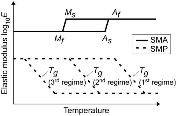
Figure 1. Three operating regimes: first regime (A_f < T_g), second regime (M_s < T_g < A_s), and third regime (T_g < M_f). Reproduced with permission from Park et al. (2012).

In the shape fixing cycle for the first operating regime, the SMP glass transition temperature range is higher than the SMA austenitic finish temperature A_f. The SMP is used to fix the position of an SMA spring in its austenitic state. In this cycle, the SMC is: (1) heated above T_g (SMP in rubbery state), (2) deformed by an initial load, and (3) cooled below T_g (M_s < T < T_g, SMP in glassy state) to its fixed state. Composite shape fixity and internal stresses are analyzed in the final fixed state when the initial load is removed.

For locking positions in a multi-way SMA actuator, the second operating regime uses an SMP with a glass transition temperature range that ideally falls between the SMA martensite start (M_s) and austenite start (A_s) temperatures. Starting with the memorized lower temperature shape, the SMC may be: (1) heated above T_g but below A_s (SMA remains martensitic); (2) deformed by a preload spring or other load; and (3) cooled below T_g to fix the deformed shape. Next, the SMC may be: (4) heated above T_g to soften the SMP, then continue to be heated above A_f to recover the initial shape of the SMA. Then, the SMC can be (5) cooled below T_g to fix the recovered shape, and further cooled to below M_f. The SMP fixes the recovered shape before the SMA transitions to martensite. In this way, the SMP can be used to fix the two-way actuator at low temperatures in either the memorized or deformed shapes.

For low temperature stiffening of an SMA in the third operating regime, the SMP glass transition temperature range is lower than the SMA martensite finish temperature M_f. In this regime, the SMA may be used in typical cycles and applications but, when cooled below T_g, the SMP adds stiffness to the current shape of the otherwise soft martensitic SMA. For example, if a counteracting spring were used with an SMA for two-way actuation, the SMA memory shape would be released before the SMP became rigid. However, the SMP would add rigidity to the deformed position at room temperature (RT), making it less sensitive to disturbances. While this regime is not examined in this paper, it could be modeled in a similar manner to the first regime, with the austenitic SMA spring force replaced by a ductile stress–strain model for a martensitic SMA.

Case I: SMP Matrix with an Embedded SMA Wire

The purpose of Case I is to analyze interfacial stresses by considering the maximum strain that results from the transition from A_s to A_f, which occurs when T > A_f. An analytical model can be used to determine the maximum interfacial stresses for designing the SMC materials and dimensions. The geometry considered is an SMA wire spring embedded in an SMP bar with rectangular cross-section. In the memorized state, the SMA wire is straight. The axial stresses in the SMA wire and interfacial shear stresses are examined analytically and using a finite element model for a compressive stress applied to the SMA wire only. The compressive stress simulates the compression that the SMA wire would experience when undergoing shape recovery, although the analysis does not consider the thermomechanical process involved in the shape memory transformation. Temperature-dependent modeling is not needed to analyze the operating regime for calculating maximum interfacial stresses. In order to evaluate maximum interfacial stresses for a limiting-case scenario, a compressive strain of 8% is considered for the SMA wire while the SMP bar remains in its rubbery state (T > T_g). NiTi alloys can exhibit superelastic strain up to 8% (McKelvey and Ritchie, 2000). Thermal expansion effects are neglected. When the SMA is in its martensitic or austenitic state, the coefficient of thermal expansion (CTE) is 6.6 × 10⁻⁶/°C or 11.0 × 10⁻⁶/°C, respectively (Dynalloy, 2013). The strain induced by CTE is negligible when compared with a compressive strain of 8%.

Axial Stress in SMA Wire and Interfacial Shear Stress

Analytical expressions for axial stress and interfacial shear stress were derived for the SMC using the shear lag model, which is widely used to analyze linear elastic stresses in short fiber composites (Hull and Clyne, 1996). The shear lag model is modified to consider a rectangular bar matrix with a traction-free boundary condition. The analytical model assumes that a stress is applied to only the ends of the wire and that both the SMA wire and SMP matrix have a cylindrical shape. Since the SMP matrix considered here is rectangular, the shear lag model is used to calculate the axial stress for the cases of a cylindrical SMP with a radius equal to the half-thickness (R_t = t/2) and the half-width (R_w = w/2) of the rectangular matrix. The axial stress of the original rectangular shape is approximated as the average of the axial stresses for the two cases.

The dotted lines in Figure 2A show the deformation caused by the axial stress σ₀. The displacement of the SMP matrix is u_R at the outer SMP radius R, and the displacement of the interface is u_r at the outer SMA radius r. The deformation u_R varies along the length because the surface boundary condition of the SMP matrix is traction-free. The detail view in Figure 2B shows the free body diagram of a single wire element and the shear strain in the matrix.

FIGURE 2

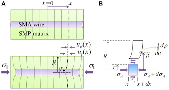
Figure 2. (A) Unloaded SMC and deformation in x–z view (shear lag model), and (B) free body diagram of a wire element and shear strain in the matrix. Reproduced with permission from Park et al. (2012).

The shear stress at the interface can be found from the force balance on the wire element shown in Figure 2B,

$\mathrm{2\pi }r\left(\mathit{dx}\right){\mathrm{\tau }}_i=-\mathrm{\pi }{r}^{\mathrm{2}}\left(d{\mathrm{\sigma }}_A\right)\to \frac{d{\mathrm{\sigma }}_A}{\mathit{dx}}=-\frac{2{\mathrm{\tau }}_i}{r}.$ (1)

By equating shear forces acting at different radii, the shear stress τ in the matrix at any radius ρ can be related to the interfacial shear stress τ_i at radius r by τ = τ_i(r/ρ). The shear strain γ in the matrix is expressed as du/dρ where u is the displacement of the matrix in the x direction. The shear strain equals the product of the shear stress τ and the shear modulus G_P. The subscripts P and A denote the SMP matrix and the SMA wire respectively,

$\frac{\mathit{du}}{d\mathrm{\rho }}=\mathrm{\gamma }=\frac{\mathrm{\tau }}{G_P}=\frac{{\mathrm{\tau }}_i}{G_P}\left(\frac{r}{\mathrm{\rho }}\right).$ (2)

The shear modulus G_P is 0.5E_P/(1 + ν_P), where E_P is the elastic modulus and ν_P is the Poisson’s ratio of the SMP. By integrating Eq. 2, the interfacial shear stress can be written in terms of the displacements u_R and u_r.

${\int }_{u_r}^{u_R}\mathit{du}=\frac{{\mathrm{\tau }}_{i}r}{G_P}{\int }_r^R\frac{d\mathrm{\rho }}{\mathrm{\rho }}\to {\mathrm{\tau }}_i=\frac{G_P\left(u_R-u_r\right)}{r\ln \left(\frac{R}{r}\right)}.$ (3)

Substitution of Eq. 3 into Eq. 1, differentiation, and application of the strains du_r/dx = ε_A = σ_A/E_A and du_R/dx = ε_P at the outer boundary gives

$\frac{d^2{\mathrm{\sigma }}_A}{d{x}^2}=\frac{n^2}{r^2}\left({\mathrm{\epsilon }}_A-{\mathrm{\epsilon }}_P\right)E_A=\frac{n^2}{r^2}\left({\mathrm{\sigma }}_A-{\mathrm{\epsilon }}_P{E}_A\right),$ (4)

where $n={\left[E_P∕\left(E_A\left(1+{\mathrm{\nu }}_P\right)\ln \left(R∕r\right)\right)\right]}^{\frac{1}{2}}$.

The top surface of the SMP matrix deforms and the strain ε_P varies along the SMA wire. The analytical solution of the second-order linear differential equation (Eq. 4) is written as:

${\mathrm{\sigma }}_A={\mathrm{\epsilon }}_P{E}_A+C_1\exp \left(\frac{n}{r}x\right)+C_2\exp \left(-\frac{n}{r}x\right),$ (5)

where the constants C₁ and C₂ are obtained by applying the boundary conditions σ_A = −σ₀ at x = ± L/2 (with L the length of the composite),

$C_1=C_2=-\left({\mathrm{\sigma }}_0+{\mathrm{\epsilon }}_P{E}_A\right)\frac{\exp \left(-\frac{\mathit{nL}}{2r}\right)-\exp \left(\frac{\mathit{nL}}{2r}\right)}{\exp \left(-\frac{\mathit{nL}}{r}\right)-\exp \left(\frac{\mathit{nL}}{r}\right)}.$ (6)

Equation 1 relates the interfacial shear stress and axial stress. After differentiation of Eq. 5 with respect to x, the shear stress can be calculated from Eq. 1,

${\mathrm{\tau }}_i=-\frac{r}{2}\frac{d{\mathrm{\sigma }}_A}{\mathit{dx}}=-\frac{n}{2}\left[C_1\exp \left(\frac{n}{r}x\right)-C_2\exp \left(-\frac{n}{r}x\right)\right].$ (7)

The specific geometry examined was a straight SMA wire with radius r = 0.375 mm embedded in the center of a rectangular SMP matrix with dimensions L = 60 mm, t = 4.2 mm, and w = 10 mm. A finite element model was constructed using COMSOL. The purpose of using FEA is to validate its consistency with analytical results and develop an analysis tool for subsequent work involving thermomechanical shape memory transformations. The FEA model uses a prescribed displacement of 2.4 mm at the ends of only the SMA wire to achieve 8% contraction of a stretched SMA wire as an upper bound for the SMA–SMP interfacial stress calculation. For the cases of the SMP radius equal to the beam half-thickness R_t and half-width R_w, the 8% strain corresponds to applied stresses of σ₀ = 5.67 GPa and σ₀ = 5.91 GPa, respectively. These large axial stresses were used for the shear lag model to replicate a limiting strain condition when examining the interfacial shear stress.

The first boundary condition du_r/dx = 8% is constant along the length of the SMA wire. The second boundary condition du_R/dx varies along the SMA wire. Data points are chosen to match the axial stresses from COMSOL simulations. The data points and curve fit are plotted in Figures 3A,B for the two SMP radii considered. In Figure 3, the horizontal axis represents the normalized position along the wire length (2x/L). The Young’s moduli of the SMA wire at high temperature and the SMP matrix at high temperature are 70 GPa and 30 MPa, respectively. The Poisson’s ratios of the SMA wire and the SMP matrix are 0.3 and 0.35, respectively.

FIGURE 3

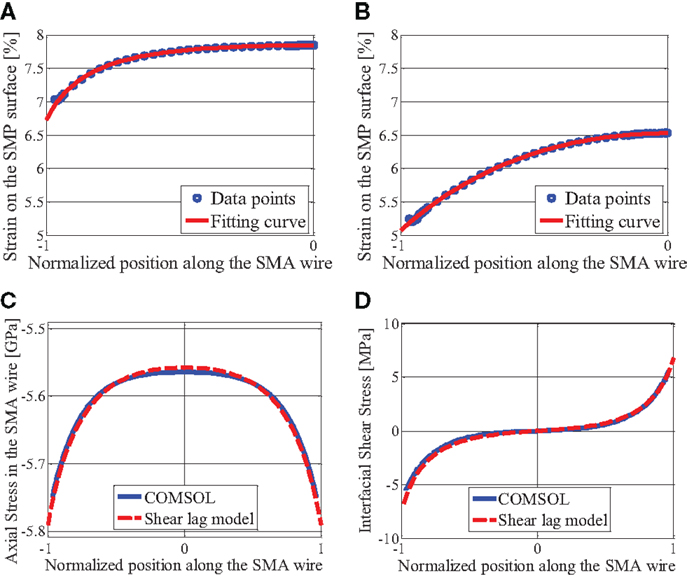
Figure 3. (A) Strain on the SMP outer surface: R = R_t, (B) strain on the SMP outer surface: R = R_w, (C) axial stress in the SMA wire, and (D) shear stress at the interface for a rectangular-shaped SMP matrix. Reproduced with permission from Park et al. (2012).

The curve fit equation is

$\frac{d{u}_R}{\mathit{dx}}={\mathrm{\epsilon }}_P=\frac{p_{\mathrm{1}}{x}^{\mathrm{2}}\mathrm{+}{p}_{\mathrm{2}}x+p_3}{x+q_1}0\le x\le 30\mathrm{mm}.$ (8)

The stress input σ₀ and boundary condition (Eq. 8) are used to calculate the constants C₁ and C₂ from Eq. 6. These constants are used for the analytical calculations of axial stress (Eq. 5) and interfacial shear stress (Eq. 7).

Finally, the axial stresses calculated using the shear lag model for radii of R_t and R_w are averaged in order to approximate the axial stress of the rectangular-shaped SMP. The predicted shear lag model results match the COMSOL simulation results, as shown in Figures 3C,D. The COMSOL stress data for the first 1 mm at both ends is not considered or shown in the figure because of stress concentrations in the simulation which are not represented by the shear lag model.

The interfacial shear stress of over 5 MPa at both ends is greater than the ultimate shear strength of Veriflex SMP, which is 0.88 MPa in the glass transition temperature state (Khan et al., 2008). Under the extreme shear stress, the SMP–SMA interface at both ends would tear.

Case II: SMP–SMA–SMP Multi-Layer Cantilever Beam (First Regime of SMC)

Case II focuses on modeling the deflection and fixity while the SMA phase remains austenitic throughout the operating regime. The geometry considered is an SMP–SMA–SMP multi-layer cantilever beam. The cantilever beam is configured with three layers as shown in Figure 4A. The beam is deflected by a downward force P applied at the end of the SMA layer, which is in its austenitic state (T > A_f). Analytical expressions are derived for deflection and shape fixity of the composite structure, normal stress in the SMA, and interfacial shear stress. These expressions are then confirmed using COMSOL finite element simulations for a selected geometry.

FIGURE 4

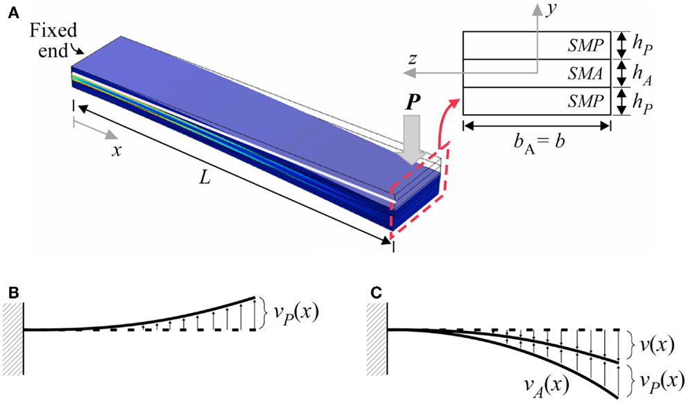
Figure 4. (A) Deflection of the SMP–SMA–SMP multi-layer composite beam and cross-section of beam, (B) calculated deflection v_P(x) of SMP-equivalent structure, and (C) initial deflection v_A(x) and final fixed deflection v(x):v_A(x) − v_P(x).

Deflection and Shape Fixity

Analytical model

The beam bending models used here assume linear elastic deformation, incompressible materials, small deflections, and that shape fixity of the SMP by itself is neglected. Initially, the point load P deforms the structure and leads to a uniformly distributed restoring force in the SMA layer. Since the SMP is then cooled to its glassy state to fix this position before the point load is removed, this restoring force is what the SMP must resist to maintain the deflected position. While the distributed restoring force acts to straighten the bent structure, due to the assumption of small deflections, the deformation of the composite from the loaded shape to the unloaded fixed state can be calculated as a distributed load applied to a straight beam.

First, the deformation of the beam is calculated for the load P applied at the free end of the beam, as shown in Figure 4A. For this model, it is assumed that the stiffness of the SMP in its rubbery state (T > T_g) is negligible compared with the stiffness of the SMA layer. As a result, the initial deformation can be calculated by considering only the SMA layer. Using standard beam bending equations, the initial deflection v_A(x) of the cantilever beam (Park et al., 2012) can be written as:

${\mathrm{\nu }}_A\left(x\right)=\frac{P}{6E_{\mathit{Aa}}{I}_A}\left(x^3-3L{x}^2\right),$ (9)

where E_Aa is the Young’s modulus of the SMA at T > A_f and I_A is the area moment of inertia of the SMA layer’s cross-section. After deflecting the beam with the SMP in its rubbery state with negligible stiffness, the beam is cooled below the SMP’s glass transition temperature T < T_g (still T > M_s) to fix the position. While Eq. 9 relates the deflection to the applied force P, the resulting shear forces F_A within the SMA can be thought of as restoring shear forces which vary as a function of deflection. Thus, from Eq. 9, the distributed shear force in the SMA that acts on the SMP and varies with deflection can be written as

$F_A=\frac{6E_{\mathit{Aa}}{I}_A{\mathrm{\nu }}_A\left(x\right)}{x^3-3L{x}^2}.$ (10)

Standard beam bending equations can be applied to composite beams by converting the beam to an equivalent geometry for a single material (Hibbeler, 1997). Here, the two SMP layers in Figure 4A are transformed into equivalent layers of SMA as shown in Figure 5A. Because the SMA layer is treated as a shear stress applied to the SMP portion of the structure, only the SMP-equivalent sections of the geometry are considered for the bending reaction (Figure 5B). The area moment of inertia about y = 0 for only the SMP-equivalent beam (Figure 5B) is (Park et al., 2012)

${I_P}_e=\frac{b_P{h}_{{}^P}^3}{6}+\frac{b_P{h}_P}{2}{\left(h_A+h_P\right)}^2,$ (11)

where h_A is the thickness of the SMA layer, h_P is the thickness of each SMP layer, and b_P is the width of the SMP layers in the SMP-equivalent geometry, given by

$b_P=b_A\left(\frac{E_{\mathit{Pl}}}{E_{\mathit{Aa}}}\right).$ (12)

E_Pl is the Young’s modulus of the SMP at low temperatures (T < T_g).

FIGURE 5

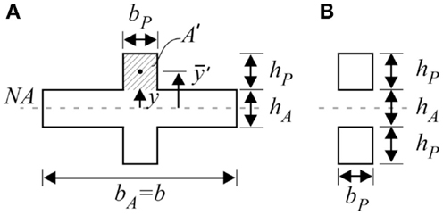
Figure 5. (A) Equivalent SMA structure for the SMP–SMA–SMP composite and (B) transformed SMP-equivalent sections.

The uniform shear force F_P is considered and the moment M = F_P(L − x) is applied to the SMP-equivalent beam. While the deflection v_P(x) is calculated for a straight SMP beam (Figure 4B), the deflection v_P(x) is considered relative to the initial deformed shape v_A(x), as shown in Figure 4C. This is reasonable due to the assumption of small deflections.

Once again applying the standard beam equations to the SMP-equivalent structure, the deflection (Park et al., 2012) can be calculated as

${\mathrm{\nu }}_P\left(x\right)=\frac{F_P}{6E_{\mathit{Aa}}{I}_{\mathit{Pe}}}\left(x^3-3L{x}^2\right),$ (13)

in terms of the equivalent geometry with area moment of inertia I_Pe.

From Eq. 13, the restoring force F_P of the SMP can be written as a function of displacement. Since v_P(x) = v_A(x)–v(x), F_P can be written in terms of the original coordinates v(x).

$F_P=\frac{6E_{Aa}{I}_{Pe}({\text{ν}}_A(x)-\text{ν}(x))}{x^3-3L{x}^2}.$ (14)

Next, equating the forces F_A and F_P, the final fixed deflection v(x) of the composite multi-layer beam relative to an initial deformation v_A(x) (Park et al., 2012) can be written as

$\mathrm{\nu }\text{(}x\mathrm{)}=\left(\frac{I_{\mathit{Pe}}}{I_A+I_{\mathit{Pe}}}\right){\mathrm{\nu }}_A\mathrm{(}x\mathrm{)},$ (15)

where ${\mathrm{\nu }}_A\mathrm{(}x\mathrm{)}$ is given from Eq. 9.

Since shape fixity is defined as the ratio of the final strain (after cooling to T < T_g and removing the initial load) to the strain due to the initial applied load (when T > T_g), the ratio of shape fixity for the SMC is

$R{F}_C=\frac{\mathrm{\nu }\left(x\right)}{{\mathrm{\nu }}_{\mathrm{0}}\left(x\right)}=\frac{I_{\mathit{Pe}}}{I_A+I_{\mathit{Pe}}}.$ (16)

Substitution of Eq. 12 into Eq. 11 gives that the area moment of inertia I_Pe for the SMP-equivalent geometry can be written as

$I_{\mathit{Pe}}=\frac{E_{\mathit{Pl}}b}{6E_{\mathit{Aa}}}\left(4h_P^3+6h_P^2{h}_A+3h_P{h}_A^2\right).$ (17)

The shape fixity of the multi-layer composite beam can also be expressed in terms of a modulus ratio R_E = E_Pl/E_Aa and a thickness ratio R_h = h_P/h_A.

$R{F}_C=\frac{I_{\mathit{Pe}}}{I_A+I_{\mathit{Pe}}}=\frac{R_E\left[8R_h^3+12R_h^2+6R_h\right]}{1+R_E\left[8R_h^3+12R_h^2+6R_h\right]}.$ (18)

COMSOL simulation

To compare the analytical models with finite element models, the material properties and geometry were selected as E_Aa = 70 GPa, E_Pl = 1.15 GPa, b_A = 10 mm, b_P = 10 mm, h_A = 1 mm, h_P = 1~10 mm, and L = 50 mm. Three loads P = 5, 25, and 50 N were considered. For the analytical results, the deflection of the composite beam was calculated from Eq. 15 and the shape fixity for the composite was obtained from Eq. 18.

While the analytical model uses a force input at a point, the COMSOL simulation used an equivalent downward stress applied to the end surface area of the SMA layer. In addition to the material property and geometry values used for the analytical model, the COMSOL simulation requires a Poisson’s ratio and density. For the SMA and SMP materials, the Poisson’s ratios are 0.3 and 0.35, and the densities are 6.45 and 1 g/cm³, respectively.

The final fixed deflection is calculated analytically using Eq. 15 for an initial load P = 5 N and plotted in Figure 6A for thickness ratios ranging from 1 to 10. Because R_h = h_P/h_A is the thickness ratio of the SMP to SMA layers, R_h = 0 corresponds to an SMP layer thickness, h_P = 0. For R_h = 0, the final fixed deflection equals the initial shape before loading since there is no SMP to fix the shape. The final fixed deflection for these same conditions was also calculated using COMSOL and plotted in Figure 6B. The analytical calculations and COMSOL simulations show good agreement.

FIGURE 6

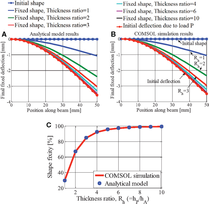
Figure 6. (A) Analytical model results and (B) COMSOL simulation results. In (A,B), the color scheme represents the initial flat shape, an initial deflection due to P = 5 N, and the final fixed deflection due to P = 5 N for six different thickness ratios from Eq. 15. (C) Shape fixity for various thickness ratios: COMSOL simulation and analytical model results. Reproduced with permission from Park et al. (2012).

Shape fixity at the tip was calculated by dividing the tip deflection of the fixed shape at each R_h by the initial tip deflection at R_h = 0. The results for the COMSOL simulation and analytical model, plotted in Figure 6C, show good agreement with less than 0.2% error in shape fixity. When R_h ≥ 6, the composite shape fixity is greater than 97%. Shape fixity is load-independent but is a function of moment of inertia as seen in Eq. 16.

Normal Stress in the SMA Layer at the Interface

Normal stresses in the SMA layer at the SMP–SMA interface are analyzed along the length of the beam. The axial normal stresses in the SMA layer at the interface can be calculated as:

${\mathrm{\sigma }}_{\mathit{Ai}}\left(x\right)=\frac{-M\left(x\right)y_{\mathit{Ai}}}{I_e}=\frac{\left(\mathit{PL}-\mathit{Px}\right)\left(h_A∕2\right)}{\frac{b_A{h}_A^3}{12}+\frac{b_P{h}_P^3}{6}+\frac{b_P{h}_P}{2}{\left(h_A+h_P\right)}^2},$ (19)

where the subscript Ai indicates points in the SMA layer at the upper SMP–SMA interface, y_Ai = h_A/2, M(x) consists of the reaction moment and force along x, and I_e is the area moment of inertia about y = 0 for the complete equivalent (all SMA) structure (Figure 5A; Park et al., 2012). The geometry and material properties are the same as those used in Section “COMSOL Simulation.” The normal stresses σ_Ai(x) are plotted and compared with COMSOL results in Figure 7A for P = 50 N and R_h = 6.

FIGURE 7

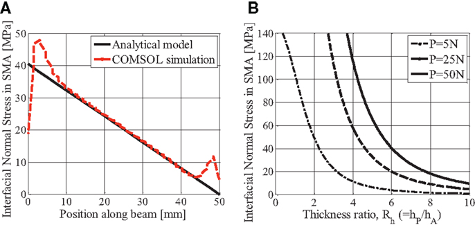
Figure 7. (A) Normal stress in SMA: analytical model and COMSOL simulation at P = 50 N and R_h = 6; (B) maximum normal stress vs. thickness ratio from analytical model. Reproduced with permission from Park et al. (2012).

As shown in Figure 7A, the analytical model predicts axial normal stresses that decrease linearly along the beam length from the fixed end to the free end, and the COMSOL simulation results show good agreement for normal stresses except at both ends of the composite beam. This is due to stress concentrations at the ends in the COMSOL simulation which are not represented in the analytical model. Figure 7B shows the maximum interfacial normal stresses in the SMA layer, which occur at the fixed end, for a range of thickness ratios and loads. So, the maximum normal stress in the SMA at the interface decreases as R_h increases. In order for the small deflection assumption used in the analytical model to be valid, the slope of the deflection curve should satisfy dv/dx < 0.1. The range of points plotted in Figure 7B satisfies this criterion but, for example, a thickness ratio of R_h = 3 with a load of 50 N does not.

The stress-induced transformation is not considered in the case of the restoring force of the SMA layer because the critical stress at the start transformation is approximately 400 MPa (McKelvey and Ritchie, 2000), which is well above the maximum interfacial normal stress shown in Figure 7B.

In addition to designing for shape fixity, the composite structure should be designed such that the maximum normal stresses in the SMA do not exceed the SMA’s yield strength. While the ultimate tensile strength of austenitic Nitinol SMA is 754–960 MPa, its tensile yield strength of 560 MPa should not be exceeded to prevent irreversible damage (TiNi Alloy Company, 2003).

Shear Stress in the SMP Layer at the Interface

Shear stresses in the SMP layer at the SMP–SMA interface are analyzed along the length of the beam. The shear force V(x) is constant along the length of the beam for a point load P applied at the end of the beam. Shear stresses in composite beams can be calculated using the shear formula (Eq. 20), where Q_Pie and I_e are calculated from the equivalent (all SMA) structure and b is the width of the original composite’s cross-section. While subscript Pi indicates points on an interface line in the SMP layer, subscript Pie denotes points on the corresponding line in the equivalent structure.

${\mathrm{\tau }}_{\mathit{Pi}}\left(x\right)=\frac{V\left(x\right)Q_{\mathit{Pie}}}{I_{e}b}=\frac{P\left(h_A+h_P\right)b_P{h}_P}{2I_{e}b}.$ (20)

$Q_{Pie}={\overline{y}}^{\prime }$ A′ where A′ is the area of the equivalent structure that is above the stress measurement point and ${\overline{y}}^{\prime }$ is the distance from the neutral axis to the center of A′, as shown in Figure 5A.

Next, the shear stress was modeled using COMSOL and plotted in Figure 8 for the entire upper SMA–SMP interface area. While the analytical model (Eq. 20) assumes constant shear stress across the width of the beam, the COMSOL results in Figure 8 show that there is a considerable variation in shear stress across the beam. This is expected for beams that are wide relative to their thickness. The analytical model results must therefore be interpreted as the average shear stress across the width of the beam rather than the maximum shear stress for each position along the beam. So, the shear stress from the COMSOL simulation was averaged for 1 mm segments along the length of the beam and plotted with the analytical model results in Figure 9A. The COMSOL simulation nearly matches the analytical model’s constant shear stress along the length of the composite beam except for stress concentrations near both ends in the COMSOL results which are not represented by the analytical model.

FIGURE 8

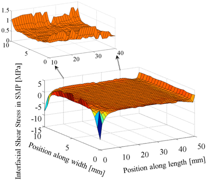
Figure 8. Interfacial shear stress: 3D plot using COMSOL simulation results. Reproduced with permission from Park et al. (2012).

FIGURE 9

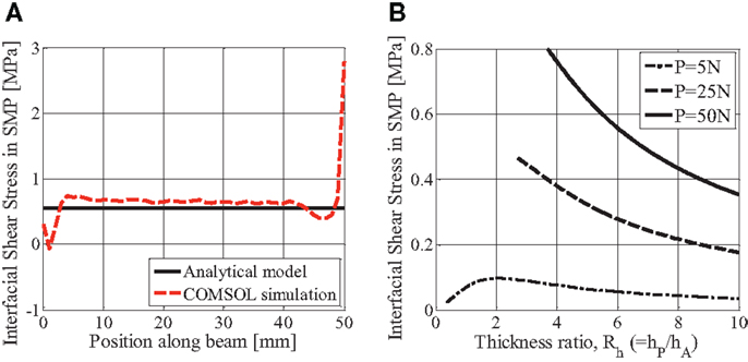
Figure 9. (A) Shear stress in SMP: analytical model and COMSOL simulation at P = 50 N and R_h = 6; (B) shear stress vs. thickness ratio from analytical model. Reproduced with permission from Park et al. (2012).

Shear stress values from the analytical model are plotted vs. thickness ratio in Figure 9B for three different loads. As seen in Eq. 20, shear stress is proportional to the applied point load. Again, the points plotted all satisfy the criterion for the small deflection assumption.

Both shear strength in the SMP and normal strength in the SMA at the interface should be considered when designing the thickness ratio. For the plotted conditions, the maximum shear stress in the SMP of 0.8 MPa occurs for P = 50 N and R_h = 3.7. In this case, the tip deflection is 3.3 mm. This maximum shear stress value is less than the ultimate shear strength of Veriflex SMP, which has been cited as 4.38 MPa at room temperature (RT) (Khan et al., 2008). At this maximum shear stress condition (P = 50 N and R_h = 3.7), the normal stress in the SMA of approximately 140 MPa (Figure 7B) is less than the 0.96 GPa ultimate tensile stress of Nitinol SMA (TiNi Alloy Company, 2003).

Case III: End-Coupled Linear SMP–SMA Two-Way Actuation System (Second Regime of SMC)

Case III focuses on the deflection and fixity at the end of the two-way actuation steps with full phase changes (pure glassy or rubbery SMP and pure austenitic or martensitic SMA) and not the transitions between the steps. The geometry considered is an end-coupled linear SMP–SMA system. First, the ability of the SMP to hold the deformed shape of the SMA is examined (first regime of SMC operation). An analytical expression for the shape fixity of the composite structure is derived which includes the SMP’s inherent shape fixity. Next, the linear SMP–SMA system is considered with an additional spring as a two-way actuation system (second regime of SMC operation), which uses the SMP to fix the actuator in two different positions at RT: martensite fixed extended and martensite fixed compressed. A numerical model predicting the strain is then validated with a two-way actuation experiment.

Analytical Model of Linear SMP–SMA System

In this section, an analytical expression for the shape fixity of a linear SMP–SMA system is derived for the first regime of operation, with the SMA remaining austenitic throughout the cycle (T > M_s). The SMP and SMA are considered to be end-coupled and act in parallel as shown schematically in Figure 10A.

FIGURE 10

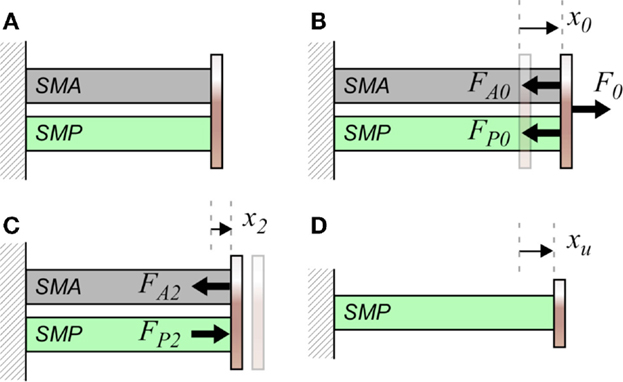
Figure 10. Linear system fixity: (A) natural state, (B) step 0 (T > T_g), (C) step 2 (T < T_g), and (D) neutral position of SMP.

In step 0 (T > T_g), an applied load F₀ causes an initial displacement x₀ as shown in Figure 10B. The force balance gives

$F_0=F_{A0}+F_{P0}=k_{\mathit{Aa}}{x}_0+k_{\mathit{Ph}}{x}_0\mathrm{and}{x}_{\mathrm{0}}=\frac{F_0}{k_{\mathit{Aa}}+k_{\mathit{Ph}}},$ (21)

where k_Aa is the stiffness of the SMA in its austenitic state. k_Pl and k_Ph are the stiffnesses of the SMP at low (T < T_g) and high (T > T_g) temperatures, respectively.

In step 1, the system is cooled below T_g (M_s < T < T_g) at constant strain. In step 2 (T < T_g), the fixed strain (at displacement x₀) is removed (Figure 10C).

An SMP has an inherent shape fixity RF_P which is defined as the ratio of the final strain after unloading ε_u and the maximum strain ε_m.

$R{F}_P=\frac{{\mathrm{\epsilon }}_u}{{\mathrm{\epsilon }}_m}=\frac{x_u}{x_0}.$ (22)

Thus, the SMP’s new “neutral” position from which the SMA strains the glassy SMP in step 2 is x_u = RF_Px₀ (Figure 10D). With the applied force removed, the system reaches equilibrium when F_A2 = F_P2.

$F_{A2}=k_{Aa}{x}_2,F_{P2}=k_{Pl}(x_u-x_2)\text{\hspace{0.17em}and\hspace{0.17em}}{x}_2=\frac{k_{Pl}}{k_{Aa}+k_{Pl}}R{F}_P{x}_0.$ (23)

By substituting x₀ from Eq. 22, the final fixed displacement can be expressed as

$x_2=R{F}_P\left(\frac{k_{\mathit{Pl}}}{k_{\mathit{Aa}}+k_{\mathit{Pl}}}\right)\left(\frac{F_0}{k_{\mathit{Aa}}+k_{\mathit{Ph}}}\right).$ (24)

The shape fixity of the end-coupled composite is therefore

$R{F}_C=\frac{x_2}{x_0}=R{F}_P\left(\frac{k_{\mathit{Pl}}}{k_{\mathit{Aa}}+k_{\mathit{Pl}}}\right).$ (25)

The shape fixity of the composite shows a relationship of an SMP’s shape fixity RF_P, the stiffness of the SMA in its austenitic state, and the stiffness of the SMP at low temperature.

Analytical Model of Linear Two-Way SMP–SMA Actuator

Next, a linear end-coupled two-way actuation system is considered which includes an additional spring element. The system operates in the second SMC regime, so the SMP’s glass transition temperature range falls between M_s and A_s. The natural lengths are defined at RT as illustrated in Figure 11A. For the numerical modeling of this system, SMA stress–strain non-linearities were modeled using the Brinson model (Brinson, 1993; DeCastro et al., 2007). SMAs in both martensitic and austenitic states have a limited stiffness in the elastic regime above which they strain at a relatively constant stress due to detwinning. In the numerical model, if an applied strain exceeds the elastic range, the force F_A for the force balance is obtained from the Brinson model which accurately predicts the non-linear stress–strain relationships in the detwinning process and the phase transformation.

FIGURE 11

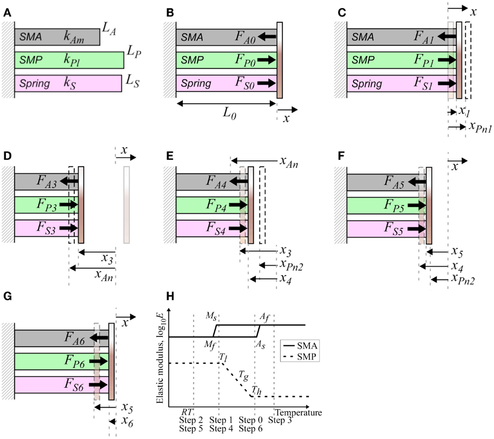
Figure 11. Two-way actuation: (A) natural states, (B) step 0, (C) step 1, (D) step 3, (E) step 4, (F) step 5, (G) step 6, and (H) steps depicted on elastic modulus and temperature diagram. (B–G) reproduced with permission from Park et al. (2012).

In the transition from twinned martensite to detwinned martensite when T < M_s,

$\mathrm{\epsilon }=\left\{\begin{array}{cc}\frac{\mathrm{\sigma }}{E_{\mathit{Am}}}\hfill & \mathrm{when}\mathrm{\sigma }<{\mathrm{\sigma }}_s^{\mathit{cr}}\hfill \\ \frac{\mathrm{\sigma }}{E_{\mathit{Am}}}+{\mathrm{\epsilon }}_L\mathrm{\xi }\hfill & \mathrm{when}{\mathrm{\sigma }}_s^{\mathit{cr}}\le \mathrm{\sigma }\le {\mathrm{\sigma }}_f^{\mathit{cr}}\hfill \\ \hfill \end{array}\right.,$ (26)

where $\mathrm{\xi }=\frac{1}{2}\cos \left\{\frac{\mathrm{\pi }}{{\mathrm{\sigma }}_s^{\mathit{cr}}-{\mathrm{\sigma }}_f^{\mathit{cr}}}\left(\mathrm{\sigma }\text{–}{\mathrm{\sigma }}_f^{\mathit{cr}}\right)\right\}+\frac{1}{2}$. Here, ${\mathrm{\sigma }}_s^{\mathit{cr}}$ and ${\mathrm{\sigma }}_f^{\mathit{cr}}$ are the critical stresses at the start of transformation and the end of transformation, respectively. E_Am is the Young’s modulus of the SMA in the martensitic state and ε_L is the maximum recoverable strain.

In the stress-induced martensite transformation when T > A_f,

$\mathrm{\epsilon }=\left\{\begin{array}{cc}\frac{\mathrm{\sigma }}{E_{\mathit{Aa}}}\hfill & \mathrm{when}\mathrm{\sigma }\le C_m\left(T-M_s\right)\hfill \\ \frac{\mathrm{\sigma }}{E}+{\mathrm{\epsilon }}_L\mathrm{\xi }\hfill & \mathrm{when}{C}_m\left(T-M_s\right)<\mathrm{\sigma }<C_m\left(T-M_f\right)\hfill \\ \hfill \end{array}\right.,$ (27)

where $\mathrm{\xi }=\frac{1}{2}\cos \left\{{}^{\pi \left(T-M_f-\frac{\sigma }{C_m}\right)}/{}_{(M_s-M_f)}\right\}+\frac{1}{2}$ and E = E_Aa + ξ(E_Am − E_Aa). E_Aa is the Young’s modulus of the SMA in the austenitic state. C_m is the stress influence coefficient in the martensitic state.

In Figure 11H, T_l and T_h denote the temperature of the SMP in full glassy and rubbery states, respectively. In Step 0 (T_g < T < A_s), an end-cap is added, with the spring and the SMP in its rubbery state acting to stretch the martensitic SMA. There is no phase change for the SMA phase and CTE changes are assumed to be negligible. The initial system length L₀ results from the force balance (Figure 11B).

$\begin{array}{ccc}\hfill F_{A0}& =k_{\mathit{Am}}\left(L_0-L_A\right),F_{P0}=k_{\mathit{Ph}}\left(L_P-L_0\right),\hfill & \hfill \\ \hfill F_{S0}& =k_S\left(L_S-L_0\right),\mathrm{and}{L}_0=\frac{k_{\mathit{Am}}{L}_A+k_{\mathit{Ph}}{L}_P+k_S{L}_S}{k_{\mathit{Am}}+k_{\mathit{Ph}}+k_S},\hfill \end{array}$ (28)

where k_Am is the stiffness of the SMA in its martensitic state.

In Step 1 (M_s < T < T_g), the system is cooled below T_g but remains above M_s. The SMP helps fix the ductile SMA’s position and the new force balance results in the position x₁ (see Figure 11C). x_Pn1 is the neutral position of the cooled SMP and RF_Pn1 is the shape fixity of the SMP.

$\begin{array}{cc}\hfill F_{A1}& =k_{\mathit{Am}}\left(L_0-L_A+x_1\right),F_{P1}=k_{\mathit{Pl}}\left(x_{\mathit{Pn}1}-x_1\right),F_{S\mathrm{1}}=k_S\left(L_S-L_0-x_1\right),\hfill \\ \hfill x_{\mathit{Pn}1}& =\left(L_P-L_0\right)\left(1-R{F}_{\mathit{Pn}1}\right),\mathrm{and}{x}_1=\frac{k_{\mathit{Am}}\left(L_A-L_0\right)+k_{\mathit{Pl}}{x}_{\mathit{Pn}1}+k_S\left(L_S-L_0\right)}{k_{\mathit{Am}}+k_{\mathit{Pl}}+k_S}.\hfill \end{array}$ (29)

In Step 2 (T = RT < M_f), the system is cooled to RT, with a minimal change in position (x₂ ≈ x₁) because the SMA was already martensitic. This step results in the first RT fixed position: martensite fixed extended.

In Step 3 (T > A_f), the system is heated through T_g then, with the SMP in its rubbery state, the SMA continues to be heated from A_s to A_f and contracts as it converts to its austenitic state (Figure 11D). The internal force of the extended SMA is calculated relative to its neutral position x_An, based on its unloaded length L_A. A force balance is again used to calculate the resulting position x₃.

$\begin{array}{cc}\hfill F_{A3}& =k_{\mathit{Aa}}\left(x_3-x_{\mathit{An}}\right),F_{P3}=k_{\mathit{Ph}}\left(L_P-L_0-x_3\right),F_{S\mathrm{3}}=k_S\left(L_S-L_0-x_3\right),\hfill \\ \hfill x_{\mathit{An}}& =L_A-L_0,\mathrm{and}{x}_3=\frac{k_{\mathit{Aa}}{x}_{\mathit{An}}+k_{\mathit{Ph}}\left(L_P-L_0\right)+k_S\left(L_S-L_0\right)}{k_{\mathit{Aa}}+k_{\mathit{Ph}}+k_S}.\hfill \end{array}$ (30)

In Step 4 (M_s < T < T_g), the system is cooled below T_g but remains above M_s. The SMP converts to its glassy state while the SMA is still contracted in its austenitic state in order to fix the position. The force in the SMP is calculated relative to its new neutral position x_Pn2, which is defined as the previous position multiplied by the shape fixity RF_Pn2 of the SMP. The position x₄ is calculated from the force balance (Figure 11E).

$\begin{array}{cc}\hfill F_{A4}& =k_{\mathit{Aa}}\left(x_4-x_{\mathit{An}}\right),F_{P4}=k_{\mathit{Pl}}\left(x_{\mathit{Pn}2}-x_4\right),F_{S\mathrm{4}}=k_S\left(L_S-L_0-x_4\right),\hfill \\ \hfill x_{\mathit{Pn}2}& =x_{3}R{F}_{\mathit{Pn}2},\mathrm{and}{x}_4=\frac{k_{\mathit{Aa}}{x}_{\mathit{An}}+k_{\mathit{Pl}}{x}_{\mathit{Pn}2}+k_S\left(L_S-L_0\right)}{k_{\mathit{Aa}}+k_{\mathit{Pl}}+k_S}.\hfill \end{array}$ (31)

In Step 5 (T = RT < M_f), the system is cooled to RT. As the SMA transforms from austenite to martensite, the SMP remains in its glassy state to maintain the compressed position. The SMP has the same neutral position as in the previous step and the position x₅ can be calculated from the force balance (Figure 11F). This step results in the second RT fixed position: martensite fixed compressed.

$\begin{array}{ccc}\hfill F_{A5}& =k_{\mathit{Am}}\left(L_0-L_A+x_5\right),F_{P5}=k_{\mathit{Pl}}\left(x_{\mathit{Pn}2}-x_5\right),\hfill & \hfill \\ \hfill F_{S5}& =k_S\left(L_S-L_0-x_5\right),\mathrm{and}{x}_5=\frac{k_{\mathit{Am}}\left(L_A-L_0\right)+k_{\mathit{Pl}}{x}_{\mathit{Pn}2}+k_S\left(L_S-L_0\right)}{k_{\mathit{Am}}+k_{\mathit{Pl}}+k_S}.\hfill \end{array}$ (32)

In Step 6 (T_g < T < A_s), the system is heated to above T_g but remains below A_s. The SMP converts to its rubbery state and allows the martensitic SMA to be stretched to its extended position. The system has returned to the same state as Step 0, with the position x₆ ≈x₀ found from the force balance (Figure 11G).

$\begin{array}{ccc}\hfill F_{A6}& =k_{\mathit{Am}}\left(L_0-L_A+x_6\right),F_{P6}=k_{\mathit{Ph}}\left(L_P-L_0-x_6\right),\hfill & \hfill \\ \hfill F_{S6}& =k_S\left(L_S-L_0-x_6\right),\mathrm{and}{x}_6=\frac{k_{\mathit{Am}}\left(L_A-L_0\right)+k_{\mathit{Ph}}\left(L_P-L_0\right)+k_S\left(L_S-L_0\right)}{k_{\mathit{Am}}+k_{\mathit{Ph}}+k_S}.\hfill \end{array}$ (33)

Experimental Testing of Linear Two-Way SMP–SMA Actuator

SMC actuator experimental prototype

A two-way SMC actuator has been designed and constructed with six SMA wires, an SMP tube, and six tuning keys as shown in Figure 12A. This geometry was designed using the two-way actuation models to maximize output strain while ensuring the ability to fix both the extended and compressed positions at RT. While the model included an optional spring element to provide a restoring force, the model results showed that the SMP in this design provided an adequate restoring force in its rubbery state without a spring. As an experimental prototype, the SMA wires are initially separated from the SMP to allow the option of controlling SMP and SMA temperatures independently; however, it is envisioned that the SMA actuators could be embedded in the SMP for future actuator designs.

FIGURE 12

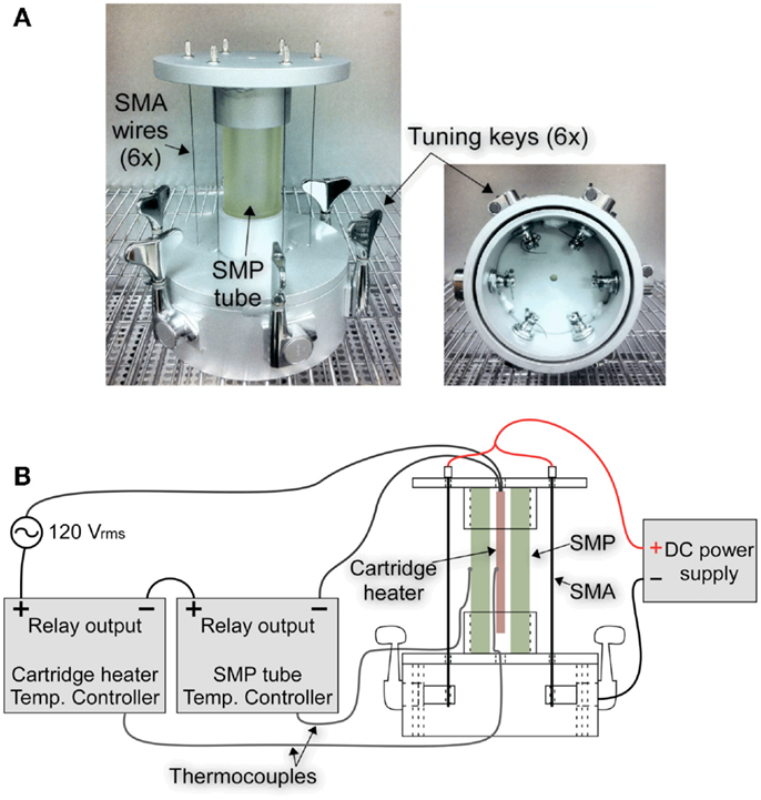
Figure 12. (A) Photo of SMC two-way actuator prototype and (B) schematic of the experimental setup.

Epoxy SMPs provide higher elastic moduli in their glassy state than polyurethane SMPs and have a broader T_g range than styrene-based SMPs (Leng et al., 2011). In addition, epoxy-based materials are easily manufactured and exhibit superior thermal and mechanical properties (Rousseau and Xie, 2010). Xie and Rousseau (2009) described an epoxy-based SMP with a tunable T_g. They showed that T_g can be decreased by increasing the mol. number of Neopentyl glycol diglycidyl ether (NGDE) and showed the shape fixity and shape recovery of epoxy samples with different mol ratios. Based on Xie and Rousseau’s formulations, an epoxy-based SMP tube was synthesized with an outer diameter of 38.1 mm (1.5″), an inner diameter of 19.05 mm (0.75″), and a length of 101.07 mm.

The Young’s modulus and shape fixity of the SMP tube were measured experimentally in an environmental chamber. The Young’s modulus was 208.88 MPa in its glassy state and 6.02 MPa in its rubbery state. The shape fixity was 97.7%.

The actuator used six Flexinol™ HT SMA wires, produced by Dynalloy Inc., with diameters of 0.51 mm and a barrel crimp applied at one end. The Young’s modulus of Flexinol is 28 GPa in its martensitic state and 83 GPa in its austenitic state.

A preload on the SMA wires is required to achieve two-way actuation with the designed strain. This preload was applied using Gotoh^® GB7 sealed tuning keys with a gear ratio of 20:1.

Finally, aluminum base and top plates were designed as shown in Figure 12A. The SMA wires passed through both plates through insulating bushings but were electrically connected at the base through the tuners and base. The SMP is mounted between the top and base plates and held in position by aluminum rings which were welded to the plates.

Test setup

Since the SMP composition has not yet been tuned to provide a transition temperature between M_s and A_s, the actuator was tested by controlling the SMA and SMP temperatures independently as shown in Figure 12B. Temperature controllers were used to control the power to a cartridge heater inside the SMP tube based on thermocouples attached to the cartridge heater and outer SMP surface. Before testing, a compliant foam insulation was wrapped around the SMP tube while leaving the SMA wires exposed to RT. The SMA wires were heated by applying up to 10 Å of direct current into the six wires connected electrically in parallel.

Test procedure

The test procedure followed the steps described in Section “Analytical Model of Linear Two-Way SMP–SMA Actuator”; however, for this testing, the temperatures of the SMP and SMA are controlled independently. For Step 0 (extended, martensite), with the SMP temperature at 70°C (above T_g) and the SMA in its martensitic state, the length of the SMA is first adjusted using the tuners to provide the desired preload and initial actuator position. The initial position L₀ was measured and the actual average unloaded SMA length L_A = 92.21 mm was measured by compressing the SMP to unload the wire.

The actuator position was measured after each of the following steps: in Step 2 (fixed extended, martensite), the SMP was cooled down to RT while the SMA remained martensitic; in Step 3a (extended, martensite), the SMP tube was heated above T_g; in Step 3b (compressed, austenite), while the SMP remained heated above T_g, the SMA wires were heated above A_f; in Step 5 (fixed compressed), while SMA wires remained heated above A_f, the SMP tube was cooled down to RT.

Test results

The actuator lengths measured after each of the steps described above are summarized in Table 1, along with the model results. The model was applied in a numerical simulation using the measured SMP Young’s modulus and shape fixity as well as the actual lengths of the SMA and SMP. Although the actuator lengths are measured as the distance between the plates, the simulation was written to account for the entire active length of the SMA, from the crimp to the tuner.

TABLE 1

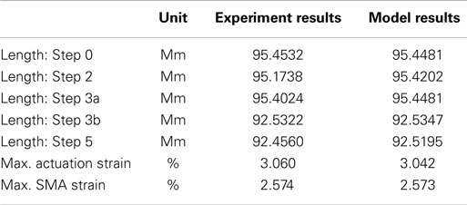
Table 1. Experiment and model results for the two-way linear SMC actuator.

As shown in Table 1, the experimental and model results for actuator strain are in very good agreement.

The maximum actuation strain is defined as the change in length between the two RT fixed positions, divided by the original actuator length. The maximum SMA strain is defined as the maximum change in SMA length divided by the original SMA length and occurs at the actuator’s original length (Step 0). For the current design, the maximum SMA strain is smaller than the maximum actuation strain because the SMA wire extends past the actuator plates, making it longer than the original actuator length. As shown in Table 1, there is very good agreement between experimental and model results for both the maximum actuation strain and the maximum SMA strain.

Conclusion

Three regimes of SMC operation have been identified that capitalize on the characteristic shape fixity of SMPs and the shape recovery of SMAs. Initial SMC analyses showed that an SMP can hold an SMA spring with minimal deflection and quantified axial stresses in an SMA wire and SMP–SMA interfacial shear stresses. Simple analytical expressions for shape fixity were derived for a multi-layer SMC beam and end-coupled linear SMC system in extension.

COMSOL simulations show good agreement with the analytical expressions for shape fixity and interfacial shear stress of a multi-layer SMC beam. A model has been developed for the two-way actuation regime of operation. A linear two-way actuator was constructed and tested with measured strain showing good agreement with model results.

In a future study, a temperature-dependent model for SMP–SMA composites will be developed over the complete cycle because it is necessary to know how the materials react as temperature changes, in particular, through the transition temperatures.

Conflict of Interest Statement

The authors declare that the research was conducted in the absence of any commercial or financial relationships that could be construed as a potential conflict of interest.

Acknowledgments

The authors wish to acknowledge the member organizations of the Smart Vehicle Concepts Center (www.SmartVehicleCenter.org), a National Science Foundation Industry/University Cooperative Research Center.

References

Bollas, D., Pappas, P., Parthenios, J., and Galiotis, C. (2007). Stress generation by shape memory alloy wires embedded in polymer composites. Acta Mater. 55, 5489–5499. doi: 10.1016/j.actamat.2007.06.006

CrossRef Full Text | Google Scholar

Brinson, L. C. (1993). One-dimensional constitutive behavior of shape memory alloys: thermomechanical derivation with non-constant material functions and redefined martensite internal variable. J. Intell. Mater. Syst. Struct. 4, 229–242. doi:10.1177/1045389X9300400213

CrossRef Full Text | Google Scholar

Brinson, L. C., and Huang, M. S. (1996). Simplifications and comparisons of shape memory alloy constitutive models. J. Intell. Mater. Syst. Struct. 7, 108–114. doi:10.1177/1045389X9600700112

CrossRef Full Text | Google Scholar

DeCastro, J. A., Melcher, K. J., Noebe, R. D., and Gaydosh, D. J. (2007). Development of a numerical model for high-temperature shape memory alloys. Smart Mater. Struct. 16, 2080–2090. doi:10.1088/0964-1726/16/6/011

CrossRef Full Text | Google Scholar

Dietsch, B., and Tong, T. (2007). A review: features and benefits of shape memory polymers (SMPs). J. Adv. Mater. 39, 3–12.

Google Scholar

Dynalloy, Inc. (2013). Nickel-Titanium Alloy Physical Properties. Available at: http://www.dynalloy.com/pdfs/TCF1140.pdf

Google Scholar

Gall, K., Mikulas, M., Munshi, N. A., Beavers, F., and Tupper, M. (2000). Carbon fiber reinforced shape memory polymer composites. J. Intell. Mater. Syst. Struct. 11, 877–886. doi:10.1106/EJGR-EWNM-6CLX-3X2M

CrossRef Full Text | Google Scholar

Hibbeler, R. C. (1997). Mechanics of Materials, 3rd Edn. Prentice Hall.

Google Scholar

Hull, D., and Clyne, T. W. (1996). An Introduction to Composite Materials, 2nd Edn. New York, NY: Cambridge University Press.

Google Scholar

Jarali, C. S., Raja, S., and Kiefer, B. (2011). Modeling the effective properties and thermomechanical behavior of SMA-SMP multifunctional composite laminates. Polymer Compos. 32, 910–927. doi:10.1002/pc.21110

CrossRef Full Text | Google Scholar

Jarali, C. S., Raja, S., and Upadhya, A. R. (2010). Constitutive modeling of SMA SMP multifunctional high performance smart adaptive shape memory composite. Smart Mater. Struct. 19, 105029. doi:10.1088/0964-1726/19/10/105029

CrossRef Full Text | Google Scholar

Keihl, M. M., Bortolin, R. S., Sanders, B., Joshi, S., and Tidwell, Z. (2005). Mechanical properties of shape memory polymers for morphing aircraft applications. Proc. SPIE, Smart Structures and Materials 2005. 5762, 143–151. doi:10.1117/12.600569

CrossRef Full Text | Google Scholar

Khan, F., Koo, J. H., Monk, D., and Eisbrenner, E. (2008). Characterization of shear deformation and strain recovery behavior in shape memory polymers. Polym. Test. 27, 498–503. doi:10.1016/j.polymertesting.2008.02.006

CrossRef Full Text | Google Scholar

Leng, J., Lan, X., Liu, Y., and Du, S. (2011). Shape-memory polymers and their composites: stimulus methods and applications. Prog. Mater. Sci. 56, 1077–1135.

Google Scholar

McKelvey, A. L., and Ritchie, R. O. (2000). On the temperature dependence of the superelastic strength and the prediction of the theoretical uniaxial transformation strain in Nitinol. Philos. Mag. A 80, 1759–1768. doi:10.1080/01418610050109455

CrossRef Full Text | Google Scholar

Park, J., Headings, L. M., Dapino, M. J., Baur, J. W., and Tandon, G. P. (2012). “Analysis of shape memory polymer-alloy composites: modeling and parametric studies,” in Proceeding of ASME 2012 Conference on Smart Materials, Adaptive Structures and Intelligent Systems. 1, 227–236. doi:10.1115/SMASIS2012-8257

CrossRef Full Text | Google Scholar

Rousseau, I. A., and Xie, T. (2010). Shape memory epoxy: composition, structure, properties and shape memory performances. J. Mater. Chem. 20, 3431–3441. doi:10.1039/b923394f

CrossRef Full Text | Google Scholar

TiNi Alloy Company. (2003). Introduction to Shape Memory Alloys. Available at: http://www.tinialloy.com/pdf/introductiontosma.pdf

Google Scholar

Tobushi, H., Hayashi, S., Hoshio, K., Makino, Y., and Miwa, N. (2006). Bending actuation characteristics of shape memory composite with SMA and SMP. J. Intell. Mater. Syst. Struct. 17, 1075–1081. doi:10.1177/1045389X06064885

CrossRef Full Text | Google Scholar

Tobushi, H., Pieczyska, E., Ejiri, Y., and Sakuragi, T. (2009a). Thermomechanical properties of shape-memory alloy and polymer and their composites. Mech. Adv. Mater. Struct. 16, 236–247. doi:10.1080/15376490902746954

CrossRef Full Text | Google Scholar

Tobushi, H., Hayashi, S., Sugimoto, Y., and Date, K. (2009b). Two-way bending properties of shape memory composite with SMA and SMP. Materials 2, 1180–1192. doi:10.3390/ma2031180

CrossRef Full Text | Google Scholar

Xie, T., and Rousseau, I. A. (2009). Facile tailoring of thermal transition temperatures of epoxy shape memory polymers. Polymer 50, 1852–1856. doi:10.1016/j.polymer.2009.02.035

CrossRef Full Text | Google Scholar