Curvature Tuning in Folded Strips Through Hyperstatic Applied Rotations

1. Introduction

Folds in thin strips are extremely localized curvatures that occur over a small length-scale. In the limit of such length to zero, the shape of the strip transforms into one with a sharp corner (Lechenault et al., 2014). Such mechanical instabilities in thin strips are often the consequence of an over-constraining environment and material mismatch (Tanaka et al., 1987; Bowden et al., 1998), such as films on foundations.

Examples of patterns generated in confined conditions (Wang and Zhao, 2015) include wrinkles (Huang et al., 2004, 2005; Guvendiren et al., 2010), creases (Hong et al., 2009; Lechenault et al., 2014), blisters, folds (Conti and Maggi, 2007; Pocivavsek et al., 2008; Bayart et al., 2014), crumples (Vliegenthart and Gompper, 2006; Deboeuf et al., 2013), and ridges (Lobkovsky et al., 1995; Lobkovsky, 1996; Lobkovsky and Witten, 1997; Audoly and Pomeau, 2010). The transitions from one to the other manifest as a consequence of the change in the boundary conditions (Holmes and Crosby, 2010; Jin et al., 2015).

Several researchers explored the mechanical snap-back and snap-through instabilities of thin structures constrained by controlled boundary conditions, both on displacements and rotations.

In Beharic et al. (2014), the authors examined the bi-stable snap-through behavior of a beam with both positive and negative curvatures. To achieve such configuration, they confined the beam with applied symmetrical rotations at both ends and end-to-end horizontal span smaller than the arc-length. By deriving a strain energy landscape, they were able to determine a critical angle at which the deformation becomes mono-stable. Such critical angle depends monotonically only on the (compression) ratio between the arc-length and the horizontal span and not on the material or thickness, (Gomez et al., 2017) by studying a very similar system, demonstrated that the speed of the snapping is lower than the prediction based on the speed of sound; in fact, even without dissipation, they discovered the existence of a slow-down near criticality.

Cazzolli and Dal Corso (2018) studied the snapping mechanisms for elastic strips without folds, generalizing the work of Beharic et al. (2014). They derived an energy release map of all the possible rotations (symmetrical and non-symmetrical) for which the strip exhibits a snap mechanism. Other recent works on snapping in over-confined thin strips include (Yu and Hanna, 2019), where they used the Kirchhoff equations for anisotropic rods to explain the stability under compression, shear, and symmetric clamping: they revealed a series of boundary conditions that can generate stable configurations. Sano and Wada (2018) instead explored a range of controlled asymmetrical boundary conditions (hinged-clamped) that generate snapping.

From the literature survey, there appears to be a considerable amount of research in confined thin sheets, especially in determining their stability. Very little yet exists on confined folded sheet. By fold, in this paper, we mean a sharp corner in the deformation (Lobkovsky, 1996; Lechenault et al., 2014).

Despite the abundance of solutions of the Euler's Elastica (Bigoni, 2012; Manning, 2014), there seems to be a lack of closed-form (or even numerical) solutions of the Elastica containing folds as we intend in this paper. Related works are (Dado et al., 2004) and (Phungpaingam and Chucheepsakul, 2018), where they studied the post-buckling response of a cantilevered column (fixed-free ends) with a rotational spring in the middle, subjected to a concentrated horizontal force at the free end. However, there is no specific connection to folds, nor the spring contains a residual dihedral angle.

A sharp corner translates into a discontinuity of the rotation of the strip. Using a numerical meshfree method initially developed for cracks, our recently published work (Barbieri et al., 2019) presented a discretization method to model thick plates with multiple folds with infinite rotational stiffness.

In this paper, we are particularly interested in how constraining a thin strip with a fold with finite rotational stiffness leads to non-zero curvatures. Also, we study how such curvatures can be tuned by modifying the applied rotations at the boundaries (Figure 1). The question of whether such shapes are stable or unstable remains a topic that requires further investigation.

FIGURE 1

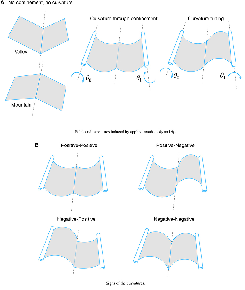
Figure 1. Curvature induced by hyperstatic confinement, and change in curvature (tuning) through applied rotations. (A) Folds and curvatures induced by applied rotations θ₀ and θ₁. (B) Signs of the curvatures.

2. Numerical Model Using Closed-Form Solutions of the Elastica

To examine which boundary conditions create curvatures in folded strips, we carried out semi-analytical simulations. Assuming invariance in the width, we modeled the strip as a plate under cylindrical bending. Therefore, instead of the Föppl-von Kármán equations, we modeled the strip as a planar, linearly elastic, unshearable, and inextensible rod, according to the Euler's theory of the Elastica.

The equilibrium equations for the Elastica are (Landau and Lifshitz, 1959; Frisch-Fay, 1962)

$\begin{array}{cc}\begin{array}{r}{\mu }^{\prime }+\frac{H_0}{B}sin\theta ̄\frac{V_0}{B}cos\theta =0\end{array}& (\mathrm{1a})\end{array}$

$\begin{array}{cc}\begin{array}{r}{\theta }^{\prime }=\mu \end{array}& (\mathrm{1b})\end{array}$

$\begin{array}{cc}\begin{array}{r}{x}^{\prime }=cos\theta \end{array}& (\mathrm{1c})\end{array}$

$\begin{array}{cc}\begin{array}{r}{y}^{\prime }=sin\theta \end{array}& (\mathrm{1d})\end{array}$

with boundary conditions

$\begin{array}{cc}\begin{array}{r}\mu (0)=\frac{M_0}{B}\end{array}& (\mathrm{2a})\end{array}$

$\begin{array}{cc}\begin{array}{r}\theta (0)={\theta }_0\end{array}& (\mathrm{2b})\end{array}$

$\begin{array}{cc}\begin{array}{r}x(0)=x_0\end{array}& (\mathrm{2c})\end{array}$

$\begin{array}{cc}\begin{array}{r}y(0)=y_0\end{array}& (\mathrm{2d})\end{array}$

where (·)′ = d/dS, with 0 ≤ S ≤ L being the curvilinear coordinate, μ is the curvature, θ is the rotation, x and y the Cartesian coordinates of the deformation, L the length of the rod, B = EI/(1 − ν²) the bending stiffness, E the Young modulus, I the second moment of area of the cross-section, ν the Poisson ratio, H₀ the applied horizontal force at S = 0, V₀ the applied vertical force at S = 0, M₀ the bending moment at S = 0, and θ₀ the rotation at S = 0, with positions x₀, y₀ at S = 0 (Figure 2A).

FIGURE 2

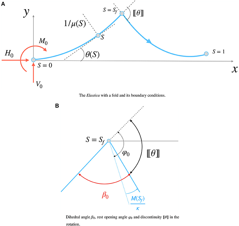
Figure 2. The Elastica with a fold at S = S_f. (A) The Elastica with a fold and its boundary conditions. (B) Dihedral angle β₀, rest opening angle φ₀ and discontinuity 〚θ〛 in the rotation.

We pass to the dimensionless form using the following normalizations:

$\begin{array}{cc}\begin{array}{r}\bar{S}=\frac{S}{L}\bar{\mu }=\mu L\bar{x}=\frac{x}{L}ȳ=\frac{y}{L}\end{array}& (3)\end{array}$

resulting in

$\begin{array}{cc}\begin{array}{r}\overline{H_0}=\frac{H_0{L}^2}{B}\overline{V_0}=\frac{V_0{L}^2}{B}\overline{M_0}=\frac{M_{0}L}{B}\end{array}& (4)\end{array}$

and the following system of non-linear ordinary differential equations [the $(\stackrel{\text{-}}{·})$ is removed for ease of notation]

$\begin{array}{cc}\begin{array}{r}{\mu }^{\prime }+H_{0}sin\theta ̄V_{0}cos\theta =0\end{array}& (\mathrm{5a})\end{array}$

$\begin{array}{cc}\begin{array}{r}{\theta }^{\prime }=\mu \end{array}& (\mathrm{5b})\end{array}$

$\begin{array}{cc}\begin{array}{r}{x}^{\prime }=\text{cos }\theta \end{array}& (\mathrm{5c})\end{array}$

$\begin{array}{cc}\begin{array}{r}{y}^{\prime }=sin\theta \end{array}& (\mathrm{5d})\end{array}$

with boundary conditions

$\begin{array}{cc}\begin{array}{r}\mu (0)=M_0\end{array}& (\mathrm{6a})\end{array}$

$\begin{array}{cc}\begin{array}{r}\theta (0)={\theta }_0\end{array}& (\mathrm{6b})\end{array}$

$\begin{array}{cc}\begin{array}{r}x(0)=x_0\end{array}& (\mathrm{6c})\end{array}$

$\begin{array}{cc}\begin{array}{r}y(0)=y_0\end{array}& (\mathrm{6d})\end{array}$

where ${(\text{·})}^{\prime }=\mathrm{\text{d}}/\mathrm{\text{d}}\stackrel{-}{S}$, with $0\le \stackrel{-}{S}\le 1$. Following standard techniques (Bigoni, 2012) of solution for Equation (5), we get

$\begin{array}{cc}\begin{array}{r}\theta (S)={\theta }_{F_0}+2\varphi (S)\end{array}& (7)\end{array}$

with θ_F0 such that

$\begin{array}{cc}\begin{array}{r}{H}_0=F_{0}cos{\theta }_{F_0}\end{array}& (\mathrm{8a})\end{array}$

$\begin{array}{cc}\begin{array}{r}{V}_0=F_{0}sin{\theta }_{F_0}\end{array}& (\mathrm{8b})\end{array}$

$\begin{array}{cc}\begin{array}{r}{F}_0=\sqrt{{H_0}^2+{V_0}^2}>0\end{array}& (\mathrm{8c})\end{array}$

and

$\begin{array}{cc}\begin{array}{r}\varphi (S)=sign(M_0)am(\alpha (S)|k^2)\end{array}& (9)\end{array}$

where am is the Jacobi amplitude function and

$\begin{array}{cc}\begin{array}{r}\alpha (S)=sign(M_0)M_{c}S+f_0\end{array}& (10)\end{array}$

with

$\begin{array}{cc}\begin{array}{r}{f}_0=F({\varphi }_0|k^2)\end{array}& (11)\end{array}$

with F is the elliptic integral of the first kind and

$\begin{array}{cc}\begin{array}{r}{\varphi }_0=\frac{{\theta }_0̄{\theta }_{F_0}}{2}\end{array}& (12)\end{array}$

$\begin{array}{cc}\begin{array}{r}{M_c}^2=\frac{{M_0}^2+2F_0(1̄cos2{\varphi }_0)}{4}\end{array}& (13)\end{array}$

$\begin{array}{cc}\begin{array}{r}{k}^2=\frac{F_0}{{M_c}^2}\end{array}& (14)\end{array}$

The Cartesian coordinates of the deformation are

$\begin{array}{cc}\begin{array}{r}x(S)=x_0+cos{\theta }_{F_0}{C}_{\varphi }(S)̄sin{\theta }_{F_0}{S}_{\varphi }(S)\end{array}& (15)\end{array}$

$\begin{array}{cc}\begin{array}{r}y(S)=y_0+sin{\theta }_{F_0}{C}_{\varphi }(S)+cos{\theta }_{F_0}{S}_{\varphi }(S)\end{array}& (16)\end{array}$

with

$\begin{array}{cc}\begin{array}{r}{S}_{\varphi }(S)={\displaystyle {\int }_0^S}sin(2\varphi (S))\mathrm{\text{d}}S=\frac{2}{M_c{k}^2}(\text{dn}(\alpha (S)|k^2)̄dn(f_0|k^2))\end{array}& (17)\end{array}$

where dn is the Jacobi dn function

$\begin{array}{cc}\begin{array}{c}{C}_{\varphi }(S)={\displaystyle {\int }_0^S}cos(2\varphi (S))\mathrm{\text{d}}S=S̄\frac{2}{M_c}(\text{sign}{\varphi }^{\prime }I(\varphi )\\ -sign{\varphi }_0^{\prime }I({\varphi }_0)+2I_{max}{n}_{{\varphi }^{\prime }\uparrow \downarrow }(S))\end{array}& (18)\end{array}$

where

$\begin{array}{cc}\begin{array}{r}I(\varphi )=\frac{1}{k^2}(F(\varphi |k^2)̄E(\varphi |k^2))\end{array}& (19)\end{array}$

where E is the elliptic integral of the second kind, I_max = I(ϕ_max) and $n_{{\varphi }^{\prime }\uparrow \downarrow }$ is the number of times from 0 to S when ϕ′ changes sign. Furthermore,

$\begin{array}{cc}\begin{array}{r}{\varphi }_{max}=\text{arcsin}\left(\frac{1}{k}\right)\end{array}& (20)\end{array}$

$\begin{array}{cc}\begin{array}{l}{\varphi }^{\prime }\left(S\right)=sign(M_0)M_{c}dn\left(\alpha (S)|k^2\right)\end{array}& (21)\end{array}$

and

$\begin{array}{cc}\begin{array}{r}\mu (S)=2{\varphi }^{\prime }(S)\end{array}& (22)\end{array}$

The strain energy of the rod is

$\begin{array}{cc}\begin{array}{l}U=\frac{1}{2}{\displaystyle {\int }_0^1}{\mu }^2\mathrm{\text{d}}S=2{\displaystyle {\int }_0^1}{{\varphi }^{\prime }(S)}^2\mathrm{\text{d}}S=2M_c^2̄2F_0{\displaystyle {\int }_0^1}{sin}^2\varphi \mathrm{\text{d}}S\\ =2M_c^2̄F_0(1̄C_{\varphi }(1))\end{array}& (23)\end{array}$

Let us now assume that a fold exists at 0 < S_f < 1. The fold is a discontinuity 〚·〛 on the rotation, with the following constitutive model (Lechenault et al., 2014)

$\begin{array}{cc}\begin{array}{r}〚\theta 〛=\theta (S_f^{+})̄\theta (S_f^{̄})=\frac{M(S_f)}{\kappa }+{\phi }_0\end{array}& (24)\end{array}$

with $S_f^{+}$ the curvilinear coordinate immediately to the right of S_f and $S_f^{-}$ the one immediately on the left (Figure 2B). The quantity κ > 0 is the rotational stiffness of the fold, and M(S_f) is the bending moment, assumed continuous in the absence of concentrated moments applied at S_f. The angle φ₀ is the rest opening angle. When φ₀ = 0, there is no fold; when φ₀ < 0 the fold is called a mountain and when φ₀ > 0 the fold is called a valley (Figure 1). The linear relationship between bending moment and dihedral angle was showed experimentally in Lechenault et al. (2014) and Jules et al. (2019) to hold for a wide range of dihedral angles. In their experiments, Lechenault and co-workers used the setup in Figure 3. The sample is clamped at one end, with a dynamometer attached to the other end. Both ends lie in the same plane. The right end can translate as the force pulls the specimen. The sample is illuminated by a laser, and the successive deformations are captured by a digital camera. In this way, it is possible to measure the dihedral angle β₀. The moment at the fold is calculated as the product of the force measured by the dynamometer and the maximum height of the profile y(S_f).

FIGURE 3

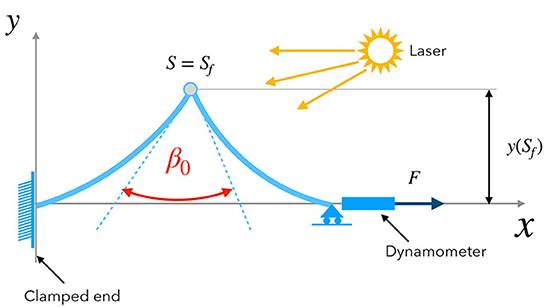
Figure 3. Experimental setup used in Lechenault et al. (2014) for the characterization of the rotational stiffness of the fold (adapted).

The geometrical meaning of φ₀ is shown in Figure 2B. The rest opening angle is related to the dihedral angle β₀ by the simple relation

$\begin{array}{cc}\begin{array}{r}{\beta }_0=\pi ̄\left({\phi }_0+\frac{M(S_f)}{\kappa }\right)\end{array}& (25)\end{array}$

The rest opening angle is a mechanical property related to the yield stress of the material of the strip (Lechenault et al., 2014): to create a sharp fold, one needs to apply an extreme deformation that generates localized and irreversible strains. Such strains, in turn, lead to high stress concentrations beyond the yield stress of the material. An estimate of the dihedral angle is (Lechenault et al., 2014)

$\begin{array}{cc}\begin{array}{r}{\phi }_0~{ϵ}_p~\frac{{\sigma }_Y}{E}\end{array}& (26)\end{array}$

where ϵ_p is the plastic strain, σ_Y the yield stress and E the Young modulus of the material composing the strip. In addition, φ₀ appears to be independent from the thickness of the strip (Lechenault et al., 2014).

To tune the curvatures, we will further assume that at least one of the following quantities is assigned:

$\begin{array}{cc}\begin{array}{r}\theta (0)={\theta }_0\theta (1)={\theta }_{1}x(1)=x_{1}y(1)=y_1\end{array}& (27)\end{array}$

which renders one or all of H₀, V₀, M₀ unknowns to be determined. The procedure to compute such unknowns is a shooting method (Press et al., 2007). Firstly, the solutions (7), (15), (16), and (22) are applied from 0 ≤ S ≤ S_f: let us call this solution μ⁻, θ⁻, x⁻, and y⁻. Then, the values θ(1), x(1), and y(1) are computed by applying the solution (7), (15), and (16) with the following boundary conditions:

$\begin{array}{cc}\begin{array}{l}\theta (S_f)={\theta }^{̄}(S_f)+\left({\phi }_0+\frac{{\mu }^{̄}(S_f)}{\kappa }\right)\end{array}& (\mathrm{28a})\end{array}$

$\begin{array}{cc}\begin{array}{r}\mu (S_f)={\mu }^{̄}(S_f)\end{array}& (\mathrm{28b})\end{array}$

$\begin{array}{cc}\begin{array}{r}x(S_f)=x^{̄}(S_f)\end{array}& (\mathrm{28c})\end{array}$

$\begin{array}{cc}\begin{array}{r}y(S_f)=y^{̄}(S_f)\end{array}& (\mathrm{28d})\end{array}$

the procedure is iterated with a non-linear solver until θ(1), x(1), and y(1) computed in this way match the conditions (27), within a certain tolerance.

3. Results

In this section we report the results of the Elastica model for strips containing folds. We examine both isostatic and hyperstatic boundary conditions. In all the numerical calculations, we set the origin of the Cartesian system to the origin of the rod, therefore x₀ = y₀ = 0.

3.1. Isostatic Boundary Conditions: no Curvature

Let us examine the case where only y(1) is assigned

$\begin{array}{cc}\begin{array}{r}y(1)=y_1\end{array}& (29)\end{array}$

Therefore

$\begin{array}{cc}\begin{array}{r}{H}_0=0M_0=0V_0=0{\theta }_0=\text{unknown}\end{array}& (30)\end{array}$

Figure 4 shows that no curvature is generated under conditions (30), regardless of the position of the fold and rotational stiffness. This configuration corresponds to the undeformed state of the folded strip when is at rest. This undeformed state depends only on the position of the fold S_f and the rest opening angle φ₀.

FIGURE 4

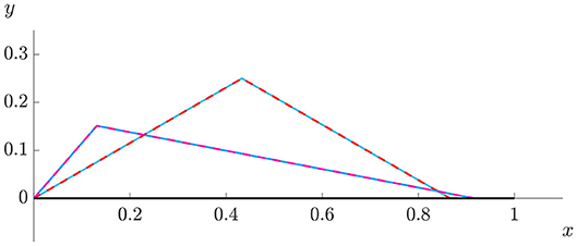
Figure 4. Deformations for S_f = 1/5 and κ = 2, and for S_f = 1/2 and κ = ∞, both with rest opening angle φ = −60° with y₁ = 0 (isostatic confinement). Blue continuous line: Elastica, red dashed line: Euler- Bernoulli (Equations 34).

3.2. Hyperstatic Boundary Conditions

In addition to condition (29), we consider cases where the boundary conditions are provided by a couple of rotations applied respectively at the start and the end of the strip:

$\begin{array}{cc}\begin{array}{r}y(1)=y_1=0\theta (0)={\theta }_0\theta (1)={\theta }_1\end{array}& (31)\end{array}$

We also impose that the end lies in the same plane as the start of the strip, therefore y₁ = 0. Under boundary conditions (31),

$\begin{array}{cc}\begin{array}{r}{H}_0=0M_0=\text{unknown }{V}_0=\text{unknown}\end{array}& (32)\end{array}$

Firstly, we consider the case of a fold with infinite rotational stiffness. By changing the applied rotations, we investigate the changes in sign of the curvatures at both sides of the fold (Figure 1B). Secondly, we repeat the same calculations for a finite rotational stiffness.

Thirdly, we isolate the effect of the rotational stiffness by varying κ for different strips under the strips under the same couple of applied rotations and the same position of the fold. We consider anti-symmetrical applied rotations.

3.2.1. Variable Applied Rotations and Rotational Stiffness

Figure 5 shows the deformations for a sheet under the same applied rotation, infinite rotational stiffness, same fold position and same rest angle.

FIGURE 5

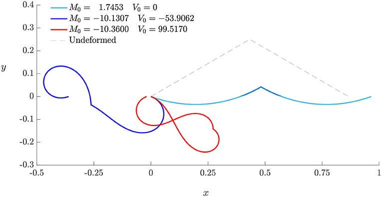
Figure 5. Non-uniqueness of the deformation for a sheet with an infinitely stiff fold positioned at S_f = 0.5, with rest angle ${\phi }_0=-60^{°}$ and applied rotations ${\theta }_0=20^{°}$, ${\theta }_1=-20^{°}$.

There exist multiple solutions, depending on the initial moment M₀ and shear force V₀. This non-uniqueness is a consequence of the non-linearity of the Elastica: in fact, the solutions (15) and (16) are periodic in space, with the period depending on M₀, H₀ and V₀ (Equation 13).

In the proceeding of the paper, we will always refer to the solution with the lowest strain energy. In fact, Equation (23) states that for the same θ₀ and θ₁, the strain energy grows with M₀ and F₀

$\begin{array}{cc}\begin{array}{r}U~{M_c}^2~{M_0}^2+F_0\end{array}& (33)\end{array}$

Having resolved this disambiguation, we now examine the changes in sign of the curvatures (Figure 1B). Figure 6A shows the curvatures at both sides of the fold for varying applied rotations at both ends. We considered θ₀ and θ₁ ranging from −|φ₀| to |φ₀|, with an increment of 1°. The fold has position S₀ = 1/2 and infinite rotational stiffness. With respect to the signs of the curvatures, there exist three regions: one where both curvatures are positive, one where both are negative and one where the curvatures have different signs.

FIGURE 6

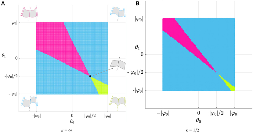
Figure 6. Signs of the curvatures at the left M₀ = μ(0) and at the right μ(1) of the fold. The rest angle is ${\phi }_0=-60^{°}$ and the position is S_f = 1/2. (A) Infinite rotational stiffness (κ = ∞). (B) Finite rotational stiffness (κ = 1/2).

Figure 6B shows a map of the signs of the curvatures for the same strip with reduced rotational stiffness κ = 1/2. We can still identify three domains, as in Figure 6A, except that the domains with the same curvatures have decreased, while the sub-regions with opposite curvature have increased. Regardless of the rotational stiffness, the three regions meet at the same point, which corresponds to the isostatic boundary conditions.

Figures 7A,B show instead the dimensionless shear force at S = 0. Both graphs are identical, with the zero shear force line being straight with equation θ₁ = −θ₀.

FIGURE 7

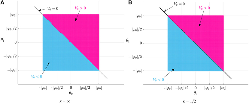
Figure 7. Sign of the shear force V₀ for a fold with rest angle φ = −60° and position S_f = 1/2. (A) Infinite rotational stiffness (κ = ∞). (B) Finite rotational stiffness (κ = 1/2).

3.2.2. Variable Rotational Stiffness for Symmetrical and Anti-symmetrical Applied Rotations

Figure 8 shows the deformations for a strip with a fold at S_f = 1/2, rest angle ${\phi }_0=-45^{°}$ and variable rotational stiffness κ. The boundary conditions are given by a fixed y-coordinate at the end y₁ = 0 and symmetrical applied rotations ${\theta }_0=-{\theta }_1=-20^{°}$. The curvature μ(S) is uniform throughout the rod, and decreases with the decrease in κ. As expected, the dihedral angle β₀ increases as κ decreases. When κ reaches a critical value κ_c, the discontinuity on the rotation disappears; below κ_c, the fold transitions from a mountain into a valley. In the limit of zero rotational stiffness, the fold becomes a perfect hinge: the deformation is equivalent to one of a flat rod, under isostatic boundary conditions, containing a fold with a rest opening angle equal to twice the applied rotation at the end.

FIGURE 8

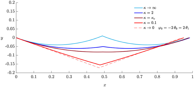
Figure 8. Deformations for variable rotational stiffness for symmetrical applied rotations ${\theta }_0=-{\theta }_1=-20^{°}$, with rest angle ${\phi }_0=-45^{°}$.

Instead, when the applied rotations are equal (anti-symmetrical rotations), the limit configuration for zero rotational stiffness is the solution of the Elastica with no folds (Figure 9).

FIGURE 9

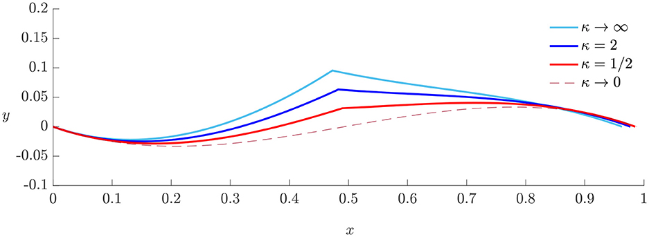
Figure 9. Deformations for variable rotational stiffness for anti-symmetrical applied rotations ${\theta }_0={\theta }_1=-20^{°}$, with rest angle ${\phi }_0=-45^{°}$.

4. Discussion

In this section, we derive a simplified analytical model to explain the numerical results obtained in section 3.

4.1. Influence of the Isostatic Confinement

In this case, the solution of the system (5) is

$\begin{array}{cc}\begin{array}{r}\mu (S)={\phi }_0\delta (S̄S_f)\end{array}& (\mathrm{34a})\end{array}$

$\begin{array}{cc}\begin{array}{r}\theta (S)={\theta }_0+{\phi }_0{H}(S̄S_f)\end{array}& (\mathrm{34b})\end{array}$

$\begin{array}{cc}\begin{array}{l}x(S)=\text{cos}{\theta }_{0}S̄(\text{cos}{\theta }_0̄\text{cos}({\theta }_0+{\phi }_0))\langle S̄S_f\rangle \end{array}& (\mathrm{34c})\end{array}$

$\begin{array}{cc}\begin{array}{l}y(S)=\text{sin}{\theta }_{0}S̄(\text{sin}{\theta }_0̄\text{sin}({\theta }_0+{\phi }_0))\langle S̄S_f\rangle \end{array}& (\mathrm{34d})\end{array}$

with δ being the Dirac delta function, ${H}$ the Heaviside function and

$\begin{array}{cc}\begin{array}{r}\langle S\rangle =\frac{S+\left|S\right|}{2}\end{array}& (35)\end{array}$

is the ramp function. The solutions in Equation (34) correspond to a piece-wise roof-like deformation, where each side of the fold is flat.

The angle θ₀ is given by

$\begin{array}{cc}\begin{array}{r}{\theta }_0=atan2\left(̄\frac{(1̄S_f)\text{sin}{\phi }_0}{S_f+\text{cos}{\phi }_0(1̄S_f)}\right)\end{array}& (36)\end{array}$

meaning that the deformation depends only upon the position of the fold S_f and the rest angle φ₀, as anticipated in Figure 4.

4.2. Influence of the Applied Rotations

For simplicity, we will also assume x₁ unassigned, making H₀ = 0. In addition, we will assume, in first instance, that the fold is infinitely stiff, meaning κ → ∞. In this case, the Elastica coincides with the classic Euler-Bernoulli beam equation:

$\begin{array}{cc}\begin{array}{r}{\mu }^{\prime }=V_0^{\infty }\end{array}& (37)\end{array}$

and the solutions for the beam are

$\begin{array}{cc}\begin{array}{r}\mu (S)=M_0^{\infty }+V_0^{\infty }S+{\phi }_0\delta (S̄S_f)\end{array}& (\mathrm{38a})\end{array}$

$\begin{array}{cc}\begin{array}{r}\theta (S)={\theta }_0+M_0^{\infty }S+V_0^{\infty }\frac{S^2}{2}+{\phi }_0{H}(S̄S_f)\end{array}& (\mathrm{38b})\end{array}$

$\begin{array}{cc}\begin{array}{r}x(S)=S\end{array}& (\mathrm{38c})\end{array}$

$\begin{array}{cc}\begin{array}{r}y(S)={\theta }_{0}S+M_0^{\infty }\frac{S^2}{2}+V_0^{\infty }\frac{S^3}{3}+{\phi }_0\langle S̄S_f\rangle \end{array}& (\mathrm{38d})\end{array}$

Assigning the following boundary conditions

$\begin{array}{cc}\begin{array}{r}\theta (0)={\theta }_0\theta (1)={\theta }_{1}y(1)=y_1=0\end{array}& (39)\end{array}$

the two unknowns V₀ and M₀ are given by

$\begin{array}{cc}\begin{array}{r}{V}_0^{\infty }=6({\theta }_0+{\theta }_1+{\phi }_0(1̄2S_f))\end{array}& (\mathrm{40a})\end{array}$

$\begin{array}{cc}\begin{array}{r}{M}_0^{\infty }=̄4\left({\theta }_0+\frac{{\theta }_1}{2}+{\phi }_0(1̄\frac{3}{2}{S}_f)\right)\end{array}& (\mathrm{40b})\end{array}$

For S_f = 1/2, the curvature will be uniform (V₀ = 0) if

$\begin{array}{cc}\begin{array}{r}{\theta }_0=̄{\theta }_1\end{array}& (41)\end{array}$

regardless of the rest angle of the fold. Such straight line in Equation (41) is observable in both Figures 7A,B.

Therefore, the curvature will be identically zero if both V₀ = M₀ = 0, which happens for

$\begin{array}{cc}\begin{array}{r}{\theta }_0={\phi }_0(1̄S_f){\theta }_1=̄{\phi }_0{S}_f\end{array}& (42)\end{array}$

The curvature in Equation (38a) is a linear function in S. Therefore, by inspecting the signs of the values at S = 0 and S = 1, it is possible to discern whether the beam has the same curvature (either positive or negative) or opposite curvatures:

$\begin{array}{cc}\begin{array}{r}\mu (0)>0\mu (1)>0\text{ same positive curvature}\end{array}& (\mathrm{43a})\end{array}$

$\begin{array}{cc}\begin{array}{r}\mu (0)<0\mu (1)<0\text{ same negative curvature}\end{array}& (\mathrm{43b})\end{array}$

$\begin{array}{cc}\begin{array}{r}\mu (0)\mu (1)<0\text{ opposite curvatures}\end{array}& (\mathrm{43c})\end{array}$

The values of μ(0) and μ(1) are

$\begin{array}{cc}\begin{array}{r}\mu (0)={M_0}^{\infty }\end{array}& (\mathrm{44a})\end{array}$

$\begin{array}{cc}\begin{array}{r}\mu (1)={M_0}^{\infty }+{V_0}^{\infty }\end{array}& (\mathrm{44b})\end{array}$

Figure 10 shows the presence of the three regions for the signs of the curvatures, as observed in Figure 6; also, there is agreement between the Euler-Bernoulli theory and the Elastica model.

FIGURE 10

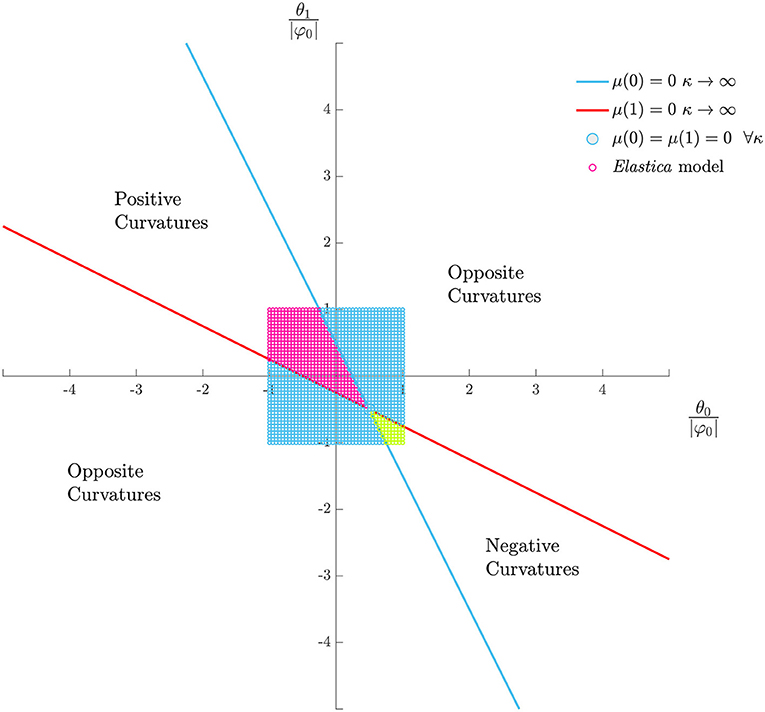
Figure 10. Curvature signs due to hyperstatic confinement through applied rotations. The fold has infinite rotational stiffness. Comparison between the Elastica model (dots) and Euler-Bernoulli beam (continuous straight lines). Pink dots: positive curvatures; green dots: negative curvatures; blue dots: opposite curvatures.

4.3. Influence of the Rotational Stiffness

Interestingly, the values in Equation (42) hold also for folds with finite rotational stiffness. In fact, when κ is finite, the solutions are

$\begin{array}{cc}\begin{array}{r}\mu (S)=M_0^{\kappa }+V_0^{\kappa }S+\left({\phi }_0+\frac{M_0^{\kappa }+V_0^{\kappa }{S}_f}{\kappa }\right)\delta (S̄S_f)\end{array}& (\mathrm{45a})\end{array}$

$\begin{array}{cc}\begin{array}{r}\theta (S)={\theta }_0+M_0^{\kappa }S+V_0^{\kappa }\frac{S^2}{2}+\left({\phi }_0+\frac{M_0^{\kappa }+V_0^{\kappa }{S}_f}{\kappa }\right){H}(S̄S_f)\end{array}& (\mathrm{45b})\end{array}$

$\begin{array}{cc}\begin{array}{r}x(S)=S\end{array}& (\mathrm{45c})\end{array}$

$\begin{array}{cc}\begin{array}{r}y(S)={\theta }_{0}S+M_0^{\kappa }\frac{S^2}{2}+V_0^{\kappa }\frac{S^3}{3}+\left({\phi }_0+\frac{M_0^{\kappa }+V_0^{\kappa }{S}_f}{\kappa }\right)\langle S̄S_f\rangle \end{array}& (\mathrm{45d})\end{array}$

where

$\begin{array}{cc}\begin{array}{r}{V_0}^{\kappa }=\frac{{V_0}^{\infty }}{1+\frac{4}{\kappa }(1̄3S_f+3{S_f}^2)}+12\frac{{\theta }_1+S_f({\theta }_0̄{\theta }_1)}{1+\frac{4}{\kappa }(1̄3S_f+3{S_f}^2)}\end{array}& (\mathrm{46a})\end{array}$

$\begin{array}{cc}\begin{array}{r}{M_0}^{\kappa }=\frac{{M_0}^{\infty }}{1+\frac{4}{\kappa }(1̄3S_f+3{S_f}^2)}+12S_f\frac{{\theta }_1+S_f({\theta }_0̄{\theta }_1)}{1+\frac{4}{\kappa }(1̄3S_f+3{S_f}^2)}\end{array}& (\mathrm{46b})\end{array}$

with ${V_0}^{\infty }$ given by Equation (40a) and ${M_0}^{\infty }$ by Equation (40b). By substituting Equations (42) into (46), the values of ${V_0}^{\kappa }$ and ${M_0}^{\kappa }$ also become zero.

In addition, for S_f = 1/2, θ₀ = −θ₁, also ${V_0}^{\kappa }=0$, which means that for opposite applied rotations, the curvature will be uniform also for folds with finite rotational stiffness.

The Euler-Bernoulli theory for soft folds in Equation (46) confirms the shrinkage of the domains with same-sign curvatures, as showed in Figure 11.

FIGURE 11

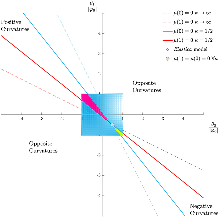
Figure 11. Curvature signs due to hyperstatic confinement through applied rotations. The fold has finite low rotational stiffness κ = 1/2. Comparison between the Elastica model (dots) and Euler-Bernoulli beam (continuous straight lines). Pink dots: positive curvatures; green dots: negative curvatures; blue dots: opposite curvatures.

The denominator in Equation (46) is always positive

$\begin{array}{cc}\begin{array}{r}\kappa +12{S_f}^2̄12S_f+4>00<S_f<1\kappa >0\end{array}& (47)\end{array}$

preventing the appearance of any singularities.

The discontinuity in rotation at the fold is given by

$\begin{array}{cc}\begin{array}{l}{〚\theta 〛}^{\kappa }=\theta (S_f^{+})̄\theta (S_f^{̄})=\frac{M(S_f)}{\kappa }+{\phi }_0\\ =\frac{{\phi }_0\kappa +{\theta }_0(6S_f̄4)+{\theta }_1(6S_f̄2)}{\kappa +12{S_f}^2̄12S_f+4}\end{array}& (48)\end{array}$

and is showed in Figure 12 for ${\theta }_0=-{\theta }_1=20^{°}$ and ${\phi }_0=-45^{°}$.

FIGURE 12

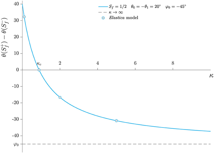
Figure 12. Discontinuity on the rotation at the fold for variable rotational stiffness. Comparison between values from Figure 8 and Equation (48).

The discontinuity becomes zero for

$\begin{array}{cc}\begin{array}{r}{\kappa }_c=4\frac{{\theta }_0}{{\phi }_0}\left(1̄\frac{3}{2}{S}_f\right)+2\frac{{\theta }_1}{{\phi }_0}(1̄3S_f)\end{array}& (49)\end{array}$

For S_f = 1/2:

$\begin{array}{cc}\begin{array}{r}{\kappa }_c=\frac{{\theta }_0}{{\phi }_0}̄\frac{{\theta }_1}{{\phi }_0}\end{array}& (50)\end{array}$

therefore, when the applied rotations are equal, then the critical rotational stiffness is zero, as in Figures 9, 12, when the applied rotations are opposite, then

$\begin{array}{cc}\begin{array}{r}{\kappa }_c=2\frac{{\theta }_0}{{\phi }_0}\end{array}& (51)\end{array}$

When θ₀ is of the same sign of φ₀, then k_c > 0 as in Figures 8, 13 and there exist a physical critical value of the rotational stiffness. Otherwise, for θ₀ = −θ₁ and φ₀ of the opposite sign, then there is no critical value, and the solution is an undeformed roof-like deformation, as determined by Equation (42).

FIGURE 13

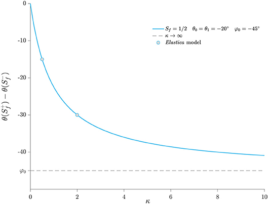
Figure 13. Discontinuity on the rotation at the fold for variable rotational stiffness. Comparison between values from Figure 9 and Equation (48).

It must be remarked, however, that even though a critical rotational stiffness for fold disappearance exists, the linear relationship in (24) might not hold for small rotational stiffness.

5. Conclusions

A thin sheet containing a fold assumes a roof-like undeformed state when confined isostatically. Instead, if confined hyperstatically, it will possess one or more curvatures. Such curvatures change according to the rotations applied at the ends of the sheet. Using the Euler's Elastica theory, we calculated the values of the applied rotations corresponding to a switch in the curvatures' signs.

We considered a fold as a discontinuity in the rotations, equal to the supplementary angle to its dihedral angle. The mechanical behavior of the fold depends upon two material properties: the rest opening angle and the rotational stiffness. The rest opening angle is a material property closely related to the yield stress; the rotational stiffness contributes to increasing the dihedral angle of the fold when subjected to a bending moment.

For infinite rotational stiffness, the dihedral angle depends only on the rest opening angle. For the signs of the curvatures before and after the fold, we can identify three regions: one where both curvatures are positive, one where they are both negative and one when they are opposite in sign. We presented a map of such occurrences according to the applied rotations; for small rotations and displacements, the numerical results agree with a simplified model based on the Euler-Bernoulli beam. Also, this map confirmed the presence of values of applied rotations for which the curvature is uniform throughout the sheet; in particular, there is one couple of applied rotations when such uniform curvature is zero. These rotations correspond to the isostatic confinement.

For folds with finite rotational stiffness, the two regions with same-sign curvatures shrink. Interestingly, there exists a critical value of the rotational stiffness when the fold disappears, meaning that the discontinuity on the rotation becomes zero. In particular, when the applied rotations are opposite in signs and the fold is a mountain, the critical value of the rotational stiffness is different from zero, and represents a transition from mountain to valley. In the limit of zero rotational stiffness, the sheet transforms into an undeformed valley with rest angle equal to twice the applied rotation at the end.

Data Availability

All datasets generated for this study are included in the manuscript and/or the supplementary files.

Author Contributions

EB designed the research, conducted the analysis, and wrote the manuscript.

Funding

EB's work was supported by the Japan Society for the Promotion of Science JSPS KAKENHI Grant Number JP18K18065.

Conflict of Interest Statement

The author declares that the research was conducted in the absence of any commercial or financial relationships that could be construed as a potential conflict of interest.

References

Audoly, B., and Pomeau, Y. (2010). Elasticity and Geometry: From Hair Curls to the Non-linear Response of Shells. Oxford: Oxford University Press.

Barbieri, E., Ventura, L., Grignoli, D., and Bilotti, E. (2019). A meshless method for the nonlinear von Kármán plate with multiple folds of complex shape - a bridge between cracks and folds. Comput. Mech. 1–19. doi: 10.1007/s00466-019-01671-w

CrossRef Full Text | Google Scholar

Bayart, E., Boudaoud, A., and Adda-Bedia, M. (2014). Tuning the ordered states of folded rods by isotropic confinement. Phys. Rev. E 89:012407. doi: 10.1103/PhysRevE.89.012407

PubMed Abstract | CrossRef Full Text | Google Scholar

Beharic, J., Lucas, T. M., and Harnett, C. K. (2014). Analysis of a compressed bistable buckled beam on a flexible support. J. Appl. Mech. 81:081011. doi: 10.1115/1.4027463

CrossRef Full Text | Google Scholar

Bigoni, D. (2012). Nonlinear Solid Mechanics: Bifurcation Theory and Material Instability. Cambridge: Cambridge University Press.

Google Scholar

Bowden, N., Brittain, S., Evans, A. G., Hutchinson, J. W., and Whitesides, G. M. (1998). Spontaneous formation of ordered structures in thin films of metals supported on an elastomeric polymer. Nature 393, 146. doi: 10.1038/30193

CrossRef Full Text | Google Scholar

Cazzolli, A., and Dal Corso, F. (2018). Snapping of elastic strips with controlled ends. Int. J. Solids Struct. 162, 285–303. doi: 10.1016/j.ijsolstr.2018.12.005

CrossRef Full Text | Google Scholar

Conti, S., and Maggi, F. (2007). Confining thin elastic sheets and folding paper. Arch. Ration. Mech. Anal. 187, 1–48. doi: 10.1007/s00205-007-0076-2

CrossRef Full Text | Google Scholar

Dado, M., Al-Sadder, S., and Abuzeid, O. (2004). Post-buckling behavior of two elastica columns linked with a rotational spring. Int. J. Nonlinear Mech. 39, 1579–1587. doi: 10.1016/j.ijnonlinmec.2004.01.003

CrossRef Full Text | Google Scholar

Deboeuf, S., Katzav, E., Boudaoud, A., Bonn, D., and Adda-Bedia, M. (2013). Comparative study of crumpling and folding of thin sheets. Phys. Rev. Lett. 110:104301. doi: 10.1103/PhysRevLett.110.104301

PubMed Abstract | CrossRef Full Text | Google Scholar

Frisch-Fay, R. (1962). Flexible Bars. London: Butterworths.

Gomez, M., Moulton, D. E., and Vella, D. (2017). Critical slowing down in purely elastic snap-through instabilities. Nat. Phys. 13, 142–145. doi: 10.1038/nphys3915

CrossRef Full Text | Google Scholar

Guvendiren, M., Burdick, J. A., and Yang, S. (2010). Solvent induced transition from wrinkles to creases in thin film gels with depth-wise crosslinking gradients. Soft Matter 6:5795. doi: 10.1039/c0sm00317d

CrossRef Full Text | Google Scholar

Holmes, D., and Crosby, A. J. (2010). Draping films: a wrinkle to fold transition. Phys. Rev. Lett. 105:038303. doi: 10.1103/PhysRevLett.105.038303

PubMed Abstract | CrossRef Full Text | Google Scholar

Hong, W., Zhao, X., and Suo, Z. (2009). Formation of creases on the surfaces of elastomers and gels. Appl. Phys. Lett. 95:111901. doi: 10.1063/1.3211917

CrossRef Full Text | Google Scholar

Huang, Z., Hong, W., and Suo, Z. (2004). Evolution of wrinkles in hard films on soft substrates. Phys. Rev. E 70:030601. doi: 10.1103/PhysRevE.70.030601

PubMed Abstract | CrossRef Full Text | Google Scholar

Huang, Z., Hong, W., and Suo, Z. (2005). Nonlinear analyses of wrinkles in a film bonded to a compliant substrate. J. Mech. Phys. Solids 53, 2101–2118. doi: 10.1016/j.jmps.2005.03.007

CrossRef Full Text | Google Scholar

Jin, L., Takei, A., and Hutchinson, J. W. (2015). Mechanics of wrinkle/ridge transitions in thin film/substrate systems. J. Mech. Phys. Solids 81, 22–40. doi: 10.1016/j.jmps.2015.04.016

CrossRef Full Text | Google Scholar

Jules, T., Lechenault, F., and Adda-Bedia, M. (2019). Local mechanical description of an elastic fold. Soft Matter. 15, 1619–1626. doi: 10.1039/C8SM01791C

PubMed Abstract | CrossRef Full Text | Google Scholar

Landau, L. D., and Lifshitz, E. M. (1959). Course of Theoretical Physics Vol 7: Theory and Elasticity. London: Pergamon Press.

Lechenault, F., Thiria, B., and Adda-Bedia, M. (2014). Mechanical response of a creased sheet. Phys. Rev. Lett. 112:244301. doi: 10.1103/PhysRevLett.112.244301

PubMed Abstract | CrossRef Full Text | Google Scholar

Lobkovsky, A., Gentges, S., Li, H., Morse, D., and Witten, T. A. (1995). Scaling properties of stretching ridges in a crumpled elastic sheet. Science 270, 1482–1485.

Google Scholar

Lobkovsky, A. E. (1996). Boundary layer analysis of the ridge singularity in a thin plate. Phys. Rev. E 53:3750. doi: 10.1103/PhysRevE.53.3750

PubMed Abstract | CrossRef Full Text | Google Scholar

Lobkovsky, A. E., and Witten, T. (1997). Properties of ridges in elastic membranes. Phys. Rev. E 55:1577. doi: 10.1103/PhysRevE.55.1577

CrossRef Full Text | Google Scholar

Manning, R. S. (2014). A catalogue of stable equilibria of planar extensible or inextensible elastic rods for all possible dirichlet boundary conditions. J. Elasticity 115, 105–130. doi: 10.1007/s10659-013-9449-y

CrossRef Full Text | Google Scholar

Phungpaingam, B., and Chucheepsakul, S. (2018). Postbuckling behavior of variable-arc-length elastica connected with a rotational spring joint including the effect of configurational force. Meccanica 53, 2619–2636. doi: 10.1007/s11012-018-0847-x

CrossRef Full Text | Google Scholar

Pocivavsek, L., Dellsy, R., Kern, A., Johnson, S., Lin, B., Lee, K. Y., et al. (2008). Stress and fold localization in thin elastic membranes. Science 320, 912–916. doi: 10.1126/science.1154069

PubMed Abstract | CrossRef Full Text | Google Scholar

Press, W. H., Teukolsky, S. A., Vetterling, W. T., and Flannery, B. P. (2007). Numerical Recipes 3rd Edition: The Art of Scientific Computing. Cambridge: Cambridge university press.

Google Scholar

Sano, T. G., and Wada, H. (2018). Snap-buckling in asymmetrically constrained elastic strips. Phys. Rev. E 97:013002. doi: 10.1103/PhysRevE.97.013002

PubMed Abstract | CrossRef Full Text | Google Scholar

Tanaka, T., Sun, S.-T., Hirokawa, Y., Katayama, S., Kucera, J., Hirose, Y., et al. (1987). Mechanical instability of gels at the phase transition. Nature 325:796. doi: 10.1038/325796a0

CrossRef Full Text | Google Scholar

Vliegenthart, G. A., and Gompper, G. (2006). Forced crumpling of self-avoiding elastic sheets. Nat. Mater. 5:216. doi: 10.1038/nmat1581

PubMed Abstract | CrossRef Full Text | Google Scholar

Wang, Q., and Zhao, X. (2015). A three-dimensional phase diagram of growth-induced surface instabilities. Sci. Rep. 5:8887. doi: 10.1038/srep08887

PubMed Abstract | CrossRef Full Text | Google Scholar

Yu, T., and Hanna, J. (2019). Bifurcations of buckled, clamped anisotropic rods and thin bands under lateral end translations. J. Mech. Phys. Solids 122, 657–685. doi: 10.1016/j.jmps.2018.01.015

CrossRef Full Text | Google Scholar