Machine Learning-Based Classification of Dislocation Microstructures

1. Introduction

One of the primary mechanisms of plastic deformation in crystalline material is the movement of dislocations. Dislocations are one-dimensional lattice defects that cause a distortion of the crystallographic lattice. The distortion results in a stress state through which dislocations interact. Once subjected to a sufficiently large stress they may start to move within a crystallographic plane, the slip plane. In addition to the interaction through their stress fields, dislocations may also form junctions or even may climb, i.e., move perpendicular to their slip plane. Thus, understanding the complex relation between dislocation microstructures and the emerging mechanical behavior is important from a fundamental point of view but is also required for designing new materials with tailored material properties. To this end, both experimental as well as numerical approaches can give important input to such developments.

In recent years, experimental methods reached the point where a three-dimensional imaging of dislocations is possible (Chen et al., 2013; Yamasaki et al., 2015). On the other side of the spectrum, due to improvements in algorithms and increasing computational power, numerical methods are able to simulate the evolution of dislocation microstructure in large specimens of up to several tens of μm (Rao et al., 2019). The drastic increase in the amount of available data sets as well as the degree of complexity of such dislocation microstructure results in a growing need for suitable algorithms and concepts for their analysis. The recent resurgence of machine learning algorithms offers a novel way for exploring this data in great detail.

Machine learning algorithms have been successfully applied in a variety of fields within materials science so far, e.g., prediction of stable compounds (Saal et al., 2013), prediction of the crystal structure (Ghiringhelli et al., 2015), band gap prediction (Dey et al., 2014), microstructure characterization (Chowdhury et al., 2016; Bostanabad et al., 2018), or material structure-property linkages (Cecen et al., 2018). The challenge of machine learning in the context of dislocation microstructures is the extraction and selection of features that are able to accurately capture the properties of both single dislocations, as well as dislocation networks. Features characterizing dislocation microstructures should capture as much of their geometrical character with as few parameters as possible. In typical dislocation dynamics simulations the microstructure is represented as a network of lines each of which requires many geometrical parameters for its definition. This makes it problematic to directly operate with these objects. We will therefore take a new approach: Based on the discrete-to-continuous (D2C) framework (Sandfeld and Po, 2015; Steinberger et al., 2016), which “borrows” the field variables of a continuum theory of dislocation dynamics. This method was already successfully used to study the emergent microstructural features of molecular dynamics simulations of plastic deformation via scratching (Gunkelmann et al., 2017) and during shock loading (Kositski et al., 2018).

In the following, we will start by introducing the main steps for converting mathematical lines into continuum field variables along with the most important simulation methods—the “discrete dislocation dynamics”—which provides the data for all subsequent analysis. We will then apply the briefly introduced machine learning algorithms to an example problem, which will allow us to study the information content of each of these field quantities. This will help to understand whether different sets of field variables suffice as features for machine learning dislocation microstructures.

2. Methods

In the following, the D2C framework is outlined as a means of converting discrete dislocation microstructures into continuous fields while retaining a variable amount of information. Then, the generation of dislocation microstructures within samples via discrete dislocation dynamics is summarized. Lastly, the machine learning algorithms used to classify the sample size based on their dislocation microstructure is given in detail.

2.1. D2C—Discrete-to-Continuous

The D2C framework (Sandfeld and Po, 2015; Steinberger et al., 2016) is based on treating dislocations as directed curves with additional physical properties, i.e., the slip plane normal, and the Burgers vector. Dislocations represent the boundary of an area over which slip displacement between two adjacent lattice planes has occurred. Dislocations can not end at arbitrary sites within the crystal, but only at free surfaces, grain boundaries, other dislocations, or other defects. A dislocation is characterized by

1. its curve parametrization, i.e., where it is in space,

2. its Burgers vector, b, which gives the magnitude and direction of the slip displacement,

3. the unit normal vector of the slip plane, n, over which the slip occurred, and

4. an orientation, represented locally by the unit line vector l, the tangent of the dislocation line.

Locally, the character of a dislocation depends on its orientation with respect to the Burgers vector. If l || b, the character is of “screw” type, if l ⊥ b, the character is of “edge” type, in all other cases it is of “mixed” type.

The so-called Kröner–Nye tensor (Nye, 1953; Kröner, 1958) is defined via

$\begin{array}{ll}\alpha ={\displaystyle \sum _{{S}}{\varrho }_{{S}}}{b}_{{S}}\otimes l_{{S}}={\displaystyle \sum _b{\displaystyle \underset{0}{\overset{2\pi }{\int }}{\displaystyle \underset{0}{\overset{2\pi }{\int }}{\varrho }_b}}}(\theta ,\phi )b\otimes l(\theta ,\phi )\text{d}\phi \text{d}\theta ,& (1)\end{array}$

where ${S}$ denotes a possible set of dislocations within a volume sharing a Burgers vector and line tangent. The integral over the spherical angles θ and φ denotes an integration over all possible orientations in three-dimensional space. It was the first attempt to describe dislocations along with structural information as continuous fields. As opposed to simplistic measures as, e.g., the total dislocation density ρ^t, which is defined as the line length per averaging volume, the Kröner–Nye tensor captures the local dislocation character in terms of the relative orientation of the line directions of the dislocations with respect to the Burgers vector. However, contributions of dislocations with opposite character cancel each other out: e.g., consider two straight line segments with the same Burgers vector but opposite line directions l⁺ and l^– = –l⁺: their average contribution is b ⊗ l⁺ + b ⊗ l^– = 0. Thus, only information about so-called “geometrically necessary” dislocations, i.e., dislocations that contribute to plastic distortion within the averaging volume, is taken into account. A number of continuum theories for predicting the evolution of dislocations are based on the Kröner-Nye tensor (Acharya and Roy, 2006; Roy et al., 2006; Xia and El-Azab, 2015).

Another theory for evolving continuous dislocation fields is the so-called higher-dimensional continuum dislocation dynamics theory developed by Hochrainer and co-workers (Hochrainer et al., 2007; Sandfeld et al., 2010). Within this theory, dislocations are represented by density and “curvature density” fields, both of which are not only a function of the spatial position r, but also of the orientations θ and φ of the dislocations. While this concept contains many important information, the extra degrees of freedom also add a high degree of complexity. This can be remedied by expanding the density and curvature fields using a Fourier series. The resulting infinite hierarchy of field equations, however, can then be truncated. For the density field of n-th order it is (Hochrainer et al., 2014; Hochrainer, 2015)

$\begin{array}{ll}{\rho }^{(n)}(r)={\displaystyle \underset{0}{\overset{2\pi }{\int }}{\displaystyle \underset{0}{\overset{2\pi }{\int }}\rho }}(r,\theta ,\phi )l{(\theta ,\phi )}^{\otimes n}\text{d}\phi \text{d}\theta ,& (2)\end{array}$

with l(r)^⊗n denoting the n-times outer product of l(r). The zeroth-order term of the series,

$\begin{array}{ll}{\rho }^{(0)}(r)={\displaystyle \underset{0}{\overset{2\pi }{\int }}{\displaystyle \underset{0}{\overset{2\pi }{\int }}\rho }}(r,\theta ,\phi )\text{d}\phi \text{d}\theta ,& (3)\end{array}$

recovers the total dislocation density at position r. The first-order term,

$\begin{array}{ll}{\rho }^{(1)}(r)={\displaystyle \underset{0}{\overset{2\pi }{\int }}{\displaystyle \underset{0}{\overset{2\pi }{\int }}\rho }}(r,\theta ,\phi )l(r)\text{d}\phi \text{d}\theta ,& (4)\end{array}$

represents the “line excess density”. If computed separately for each slip system, it is the “geometrically necessary” dislocation density for this slip system. The second-order term,

$\begin{array}{ll}{\rho }^{(2)}(r)={\displaystyle \underset{0}{\overset{2\pi }{\int }}{\displaystyle \underset{0}{\overset{2\pi }{\int }}\rho }}(r,\theta ,\phi )l(\theta ,\phi )\otimes l(\theta ,\phi )\text{d}\phi \text{d}\theta ,& (5)\end{array}$

denotes the “line direction density”. If computed separately for each slip system in a coordinate system that is based on the Burgers vector of that slip system, it can be interpreted as the density of edge- and screw-type dislocation character. The theory based on these fields and an additional field—the curvature density of the dislocations—is able to represent the kinematics of dislocation motion for simplified single slip situations, which was shown by Sandfeld and Po (2015) by comparison with discrete dislocation dynamics simulations.

Numerically, the computation of the fields based on discrete dislocation data is carried out in the following way. The subvolume of interest within a specimen is discretized into voxels Ω_i. Microstructure features may then be extracted for each voxel by treating each dislocation as a parameterized curve c(u) via

$\begin{array}{ll}\frac{1}{V_{{\Omega }_i}}{\displaystyle \sum _{c\in {\Omega }_i}}{\displaystyle \underset{{{L}}_{{\Omega }_i}^c}{\int }}{f}_c(u)\text{d}u,& (6)\end{array}$

where u is the arc length, and V_Ωi is the volume of the voxel Ω_i. f_c(u) denotes a field specific term that relies on the geometrical and physical properties of the dislocation curve c. An overview of the continuous fields used as features and their corresponding term for f_c(u) is compiled in Table 1.

TABLE 1

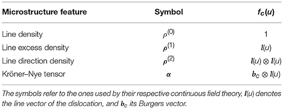
Table 1. Features extracted from the dislocation microstructures following Equation (6).

2.2. The Discrete Dislocation Dynamics Method

The discrete dislocation dynamics methods represent dislocation as polygonal chains, i.e., an ordered sequence of segments. Forces acting on those segments, or their vertices, due to other dislocations, external load, and/or image forces due to surfaces are computed, and subsequently used to move the dislocations according to a velocity law. Additionally, local rules are implemented to take dislocation reactions like cross-slip or junction formation into account. A velocity law combined with the local rules can then be time-integrated to update the dislocation positions.

2.3. Data Generation and Simulation Set Up

The generation and evolution of dislocation microstructures were performed using the MODEL discrete dislocation dynamics code (Po et al., 2012; Po and Ghoniem, 2014). Cube-shaped copper samples with edge lengths of 30, 60, and 90 nm were filled with dipolar edge loops that were randomly placed on all slip systems up to a total dislocation density of ≈ 5 × 10¹⁶ m⁻². Throughout the simulations, the effect of open boundaries on the dislocations was taken into account and dislocations were allowed to exit the samples. Subsequently, these random structures were relaxed without application of an external stress.

Due to the open boundaries image forces act on the dislocations that attract them to the free surfaces where parts of them leave the specimen. The attraction is stronger the closer the dislocation is to the surface. Therefore, we expect the dislocation density ρ⁽⁰⁾ to be smaller at the boundaries of the specimen. Furthermore, if unhindered, the remaining part of the dislocation should be oriented perpendicular to the surface. This preference of dislocation line direction should show in the line direction density ρ⁽²⁾. Thus, the region close to the surfaces should exhibit dislocation microstructure features that are different from that of the center of the sample. For simplicity, formation of junctions was not considered in the present study, which resulted in a large simulation speedup allowing to generate more samples.

Overall, 306 realizations of the 30 nm specimen, 238 of the 60 nm specimen, and 207 of the 90 nm specimen were generated. Due to the relatively small number of samples that can be investigated in this study, slip system specific dislocation densities would be prone to overfitting. Instead, only the line directions of each dislocation within the subvolume are taken into account regardless of the slip system. The local deformation character of the dislocation ensemble is therefore only considered by the Kröner–Nye tensor due to it taking the Burgers vector into account.

Due to the different size of the samples, the dislocation arrangement close to the surface can be expected to differ between the sample sizes. Therefore, we ask the following question: Can a machine learning model be trained to classify the sample size based on the dislocation microstructure within a subvolume at the surface of the specimen?

A 30 × 30 × 30 nm subvolume at the center of the side oriented toward the negative x-direction was chosen, see Figure 1. For the 30 nm sample, the whole volume is thus taken into account, including all the surfaces. In the larger specimen, the subvolume only contained one free surface. Assuming that the microstructure features are able to capture the characteristics of the microstructure, the classification of the 30 nm sample should be easier than the classification of the 60 nm, and 90 nm samples.

FIGURE 1

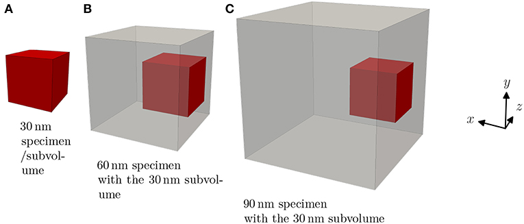
Figure 1. Sample geometries considered in this work. The subvolumes used for the classification of the specimen size are shown in red. Their size is 30 nm for all specimen sizes. (A) 30 nm specimen/subvolume. (B) 60 nm specimen with the 30 nm subvolume. (C) 90 nm specimen with the 30 nm subvolume.

2.4. Machine Learning of Dislocation Microstructures

Machine learning algorithms rely on the description of samples by common features, that are then typically used for classification, regression, and/or clustering. A feature is a measurable property of a sample that provides information about a sample and puts it into relation with other samples. Classification describes the procedure of trying to infer a label for one or several samples based on the features of other samples with a known label. In this work, a Gaussian naive Bayes classifier is used, which is briefly explained in the following. For more details, see Domingos and Pazzani (1997), and Hand and Yu (2001).

Bayes' theorem states that the probability P of a sample with features $\widehat{X}$ belonging to class y_i is given by

$\begin{array}{ll}P(y=y_i|X=\widehat{X})=\frac{P(X=\widehat{X}|y=y_i)P(y=y_i)}{P(X=\widehat{X})}.& (7)\end{array}$

Here, P(A | B) denotes the conditional probability of A under the condition B. The predicted class then is the class for which this probability is the highest considering the given feature vector. Thus, the denominator of Equation (7) becomes irrelevant, as it does not depend on the class. Both, P(y = y_i)—the probability that the class is y_i—and $P(X=\widehat{X}|y=y_i)$—the probability that the features are $\widehat{X}$ given that the class is y_i—are results of the supervised learning procedure. The former is computed via the number of times class y_i was observed within all training data with respect to all training data. The latter is assumed to be modeled by a gaussian distribution for each occurring class individually, with the mean and standard deviation being computed from the features of specimen belonging to that class within the training dataset.

A simple example of the Gaussian naive Bayes classification can be seen in Figure 2. The samples shown as dots were used to train a Gaussian naive Bayes classifier. Subsequently, the feature space was sampled for its classification areas and they are shown accordingly. Interfaces between these areas are called decision boundaries and represent ambiguous feature combinations.

FIGURE 2

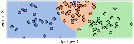
Figure 2. Graphical representation of a classification algorithm using two features to classify samples into three distinct classes, represented by their color. A Gaussian naive Bayes classifier was trained using the samples seen as dots and subsequently the areas, whose feature combination would lead to a specific classification, was colored accordingly. It can be seen that not all samples would be classified correctly even though they have been part of the training data.

In this work features used for machine learning are the microstructure features in the subvolumes of each sample. This is done to make them comparable w.r.t the voxel size and position of the features. If, instead, we used the whole specimen size, the data would not be comparable.

The performance of classification models is then measured by cross-validation and the accuracy score, i.e., the number of correctly labeled samples divided by the total number of samples that were labeled. Additionally, so-called confusion matrices may be computed. They reveal details of the mislabeling by keeping track of the true label and the one predicted by the machine learning model.

To measure the influence of the spatial resolution and its interplay with the different features on the classification score, different combinations of spatial discretizations and density features are applied. Each subvolume was subdivided into up to 8 segments along each direction, resulting in up to 512 voxels Ω_i. Subsequently, the features were computed within each of those voxels using the D2C framework.

For each combination of spatial discretization and features, 30 shuffled stratified 5-fold cross-validations were performed to determine the average accuracy scores and confusion matrices of the models. Throughout this work, the Python packages NumPy (Oliphant, 2015) version 1.16.0, and scikit-learn (Pedregosa et al., 2011) version 0.20.2 were used.

3. Results

Dislocation structures in specimens of three different sizes are created using the open source discrete dislocation dynamics code MODEL according to the relaxation procedure outlined in the previous section. Examples for such dislocation structures within a subvolume are shown in the top row of Figure 3. All subvolumes exhibit a depletion of dislocations close to the surface. This behavior is most pronounced for the 30 nm specimens. Applying the D2C coarse-graining to the discrete dislocation structure we obtain continuous dislocation dynamics (CDD) field data. To be able to directly compare the microstructures of different specimen sizes, we cut samples of equal sizes from each specimen size (compare Figure 1). Typical density distributions for different specimen sizes and with two different discretizations are illustrated in Figure 3.

FIGURE 3

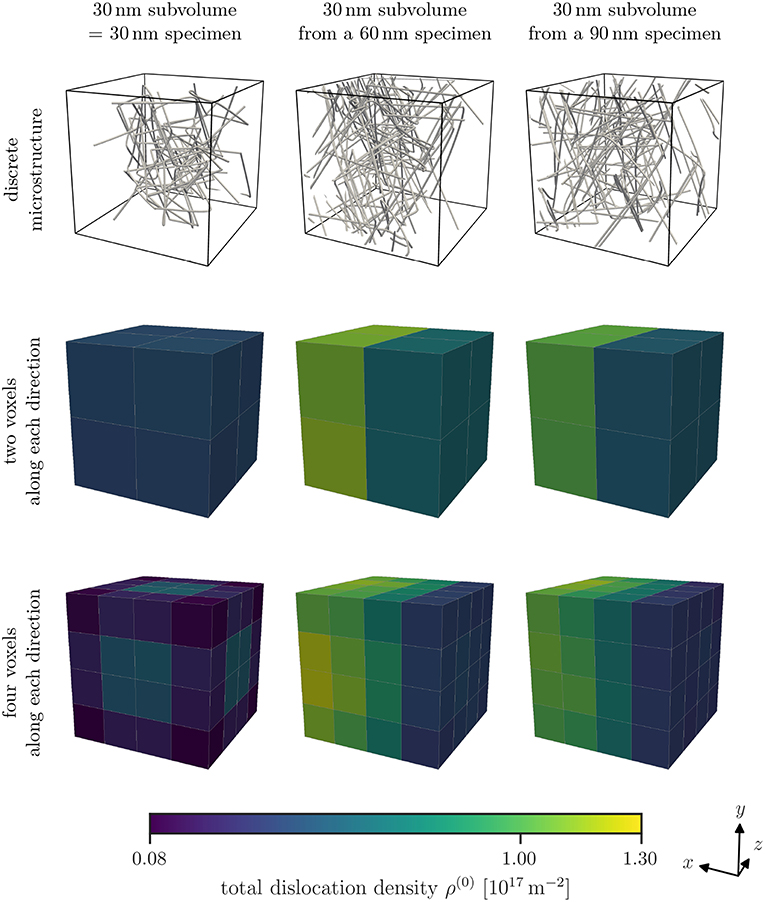
Figure 3. Examples of discrete microstructures found within the inspected subvolumes of the different specimen sizes can be seen in the top row. Note that the size of the subvolumes is the same, but the specimen they were taken from are different (see Figure 1). The open surface common to all subvolumes irrespective of the specimen size is in negative x-direction, in this case, to the right. Average total dislocation density ρ⁽⁰⁾ for each studied specimen size and two or four voxels per direction as discretization are shown in the bottom rows.

The overall total dislocation density of the 30 nm specimens is smaller than that of the 60 nm and 90 nm specimens. Furthermore, the smallest sample also shows a highly symmetric density morphology, while the average total dislocation density in the larger samples exhibit a gradient, i.e., an increase in direction of the negative x-direction, with smaller density at the free surface at the right. Along the other two directions no gradient can be observed. This is a result of the way how we cut samples out of the specimens of different sizes: only the smallest sample has free surfaces everywhere, while the samples from the 60 nm and 90 nm specimens have only one free surface, i.e., the one with outwards normal pointing into positive x-direction.

Having presented general observations of the microstructure, the results of the machine learning model are presented in the following.

Figure 4 shows the average accuracy scores computed from the machine learning model. They were obtained for different combinations of microstructure features and for different coarse-graining voxel sizes. These particular combinations are commonly used in continuous dislocation simulations models. It can be seen that in particular for large voxel sizes (≤ 3 × 3 × 3 voxel) the accuracy score of the Kröner–Nye tensor is low compared to those obtained for the CDD field variables. For higher resolutions, the Kröner–Nye tensor α scores higher than the total dislocation density ρ⁽⁰⁾ but is still performing not as good as using more than one CDD feature at the same time. Using (combinations of) the CDD field variables from Hochrainer's CDD theory, the general trend is that a larger number of involved fields leads to a better or at least comparable score. Using the direction line density ρ⁽²⁾ in addition to the excess line density ρ⁽¹⁾ and the total density ρ⁽⁰⁾ leads to a significant improvement in the accuracy score (green curve in Figure 4).

FIGURE 4

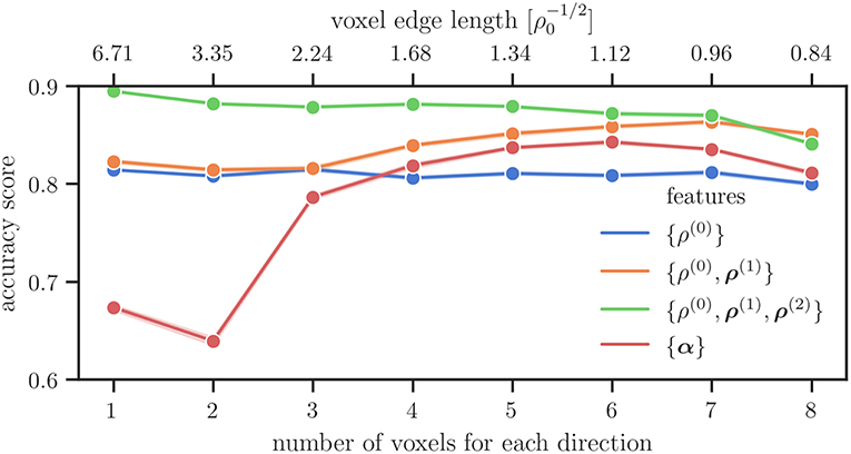
Figure 4. Average accuracy score of the microstructure features in combinations that are used within their respective theories over the number of voxels along each axis used for the spatial discretization.

To study in more detail what the influence of different features is we investigate the accuracy score for only using a single feature and for combinations of two features in Figure 5, on the left and on the right, respectively. If only one voxel is considered for the spatial discretization, the total line density {ρ⁽⁰⁾} is the best predictor of the sample size, followed by the direction line density {ρ⁽²⁾}. The latter starts to perform better for resolutions of more than one voxel for each direction. The excess line density {ρ⁽¹⁾} performs better with higher resolution, performing better than the total dislocation density {ρ⁽⁰⁾} for more than four voxels per axis, and better than the direction line density {ρ⁽²⁾} for more than seven voxels per axis. Field combinations involving ρ⁽²⁾ perform better than those without it, the exception being the highest resolution of eight voxels per axis. For low resolutions the combination {ρ⁽⁰⁾, ρ⁽²⁾} is more accurate than the combination {ρ⁽¹⁾, ρ⁽²⁾}. For more than two voxels per direction the accuracy of the two becomes comparable.

FIGURE 5

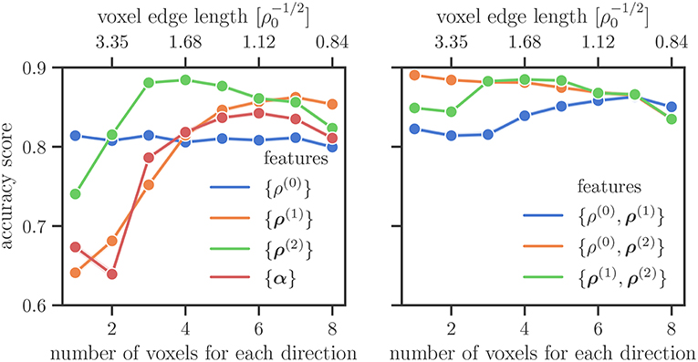
Figure 5. Average accuracy score on the test data set for different features and their combinations. In the right plot the lines for {ρ⁽⁰⁾, ρ⁽²⁾} and {ρ⁽¹⁾, ρ⁽²⁾} coincide for a larger number of voxels for each direction.

Confusion matrices for only using the total dislocation density as feature are shown for different resolutions in Figure 6. There, the vertical axis shows the real specimen size and the horizontal axis is the size inferred by the classification algorithm. One observes that the 30 nm samples are always labeled correctly: each matrix has a “1” in the top left. Larger samples are mislabeled more often, with a stronger tendency of mislabeling the specimen as a too small specimen, i.e., the 90 nm sample is more often classified as 60 nm than the other way around. This effect is less pronounced for higher resolutions. At the same time the accuracy of correctly labeling the 60 nm samples slightly decreases.

FIGURE 6

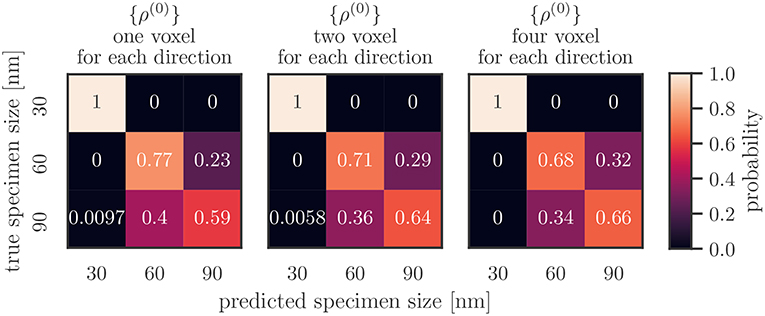
Figure 6. Average confusion matrices for different resolutions taking only the total dislocation density {ρ⁽⁰⁾} as feature into account.

The confusion matrix of the best performing combination of features and resolutions, {ρ⁽⁰⁾, ρ⁽¹⁾, ρ⁽²⁾}, for one voxel, is shown in Figure 7 on the right. The predicted size of 30 nm samples perfectly matches the actual size. Sixty and ninety nanometer samples are predicted correctly with an accuracy of above 0.8. Specimens that could not be predicted correctly were never labeled as 30 nm, and the degree of false labelings of the two larger samples (i.e., identifying a 60 nm specimen as a 90 nm and vica versa) is balanced.

FIGURE 7

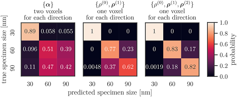
Figure 7. Average confusion matrix on the test data set of the features {α}, {ρ⁽⁰⁾, ρ⁽¹⁾}, {ρ⁽⁰⁾, ρ⁽¹⁾, ρ⁽²⁾} for low resolutions per axis. The first combination performed worst, the last best out of all investigated combinations.

The combination of the Kröner–Nye tensor and a resolution of two voxel per direction performed worst out of the investigated combinations. Its confusion matrix is shown in Figure 7 on the left. While specimens of size 30 nm are not predicted perfectly, they still remain those that are most accurately predicted. False predictions are not limited to just the next smaller or larger sizes, as roughly 5 % of 30 nm samples are classified as 90 nm, and roughly 11 % the other way around. Slightly more than half of the 60 and 90 nm samples are classified as 60 nm.

These two extreme cases also summarize all other combinations of continuous fields and resolution: The 30 nm specimens are much more reliably classified than the larger specimens. If larger specimens are mislabeled, the tendency is that the 90 nm specimen is classified as being 60 nm more often than vice-versa.

4. Discussion

4.1. Accuracy of Classifying 30 nm vs. 60 nm, and 90 nm

The confusion matrices show that there is a striking difference in the accuracy with which subvolumes of 30 nm specimen are classified compared to the larger specimen. The reason for this is that the subvolumes of 30 nm specimens have six free boundaries, whereas the subvolumes of larger specimen only have one. As seen in Figure 3, this leads to distinct density features for the 30 nm specimens/subvolumes. On the one hand, the overall dislocation density is lower compared to the larger specimens. As dislocations are attracted to free surfaces through which they can leave the specimen, more free surfaces closer to the subvolume result in a lower density. On the other hand, there is no gradient of the dislocation density like in the larger specimen. While the dislocations close to the free surfaces in the larger specimen are able to leave the samples, dislocations closer to the center of the specimen can not. On average, this leads to a large density gradient in the subvolumes of larger samples. These are the features likely learned by the model and lead to a high accuracy in distinguishing the 30 nm subvolumes from larger ones, regardless of the resolution.

Classification of subvolumes of the larger specimen is less accurate as their basic features are the same: both have one free surface, while their other surfaces are inside the specimen. However, the distance of the “inner” subvolume surfaces to the specimen surfaces is different for the 60 nm and the 90 nm samples. This likely leads to more subtle differences in the dislocation microstructure that have to be represented as features for the machine learning algorithm to recognize them. For this, two options seem to be available:

• Increasing the resolution while keeping the microstructure features the same. This way, lower order features are not “averaged out” over large volumes. Figure 4 together with the confusion matrices seen in Figure 6 show that this is one way to increase the accuracy of the model.

• Using higher order microstructure features while keeping the resolution the same. This way, more details of the microstructure are captured in the same averaging volumes. Figure 4 and the confusion matrices seen in Figure 7 confirm that this is also viable for increasing the accuracy.

Both ways also alleviate the asymmetry in mislabeling subvolumes of the larger specimen. If one looks at the “feature efficiency,” i.e., how many features are used to get the best accuracy, including more information via higher order terms of Hochrainer's CDD theory is the better solution.

4.2. Resolution and Features

Is it possible to identify a simple or generic recipe that helps to choose the “right” resolution or “correct” number of features? To answer this question the accuracy scores for all feature combinations and numbers of voxels for each direction are summarized in Figure 8.

FIGURE 8

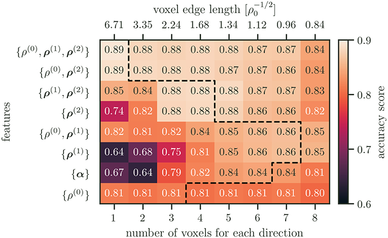
Figure 8. Accuracy scores for all feature combinations and resolutions. The features are ordered by their maximum accuracy score, with the best performing features on top. The dashed line indicates the point after which an increase in resolution results in worse performance.

When only using one microstructure feature set, the total dislocation density ρ⁽⁰⁾ performs best for low resolutions. While the performance of ρ⁽⁰⁾ remains rather unchanged for higher resolutions, other single microstructure features perform better at different resolutions. This can be explained by the length scales of the features compared to the spatial resolution. If there is only a single voxel, then the details that are captured by ρ⁽²⁾ are averaged out. The performance increases as the resolution gets higher up to a point of about two average dislocation spacings. At this point the length scale of the details represented by ρ⁽²⁾ likely coincides with the resolution and leads to good performance.

The poor performance for the line excess density ρ⁽¹⁾ and the Kröner–Nye tensor α at resolutions below one average dislocation spacing can furthermore be explained by the chosen dislocation configuration. Both measures are only able to describe dislocation configurations that show an excess of a particular dislocation type that ultimately leads to a plastic distortion of the lattice. In our example, the average dislocation character is balanced, i.e., on average there is no plastic distortion in the specimen. Thus, the local formation of substructures of different “character excess” is averaged out if the resolution is chosen too low. As the resolution is increased and approaches a comparable scale, the performance of these measures increases and, in some cases, even surpasses that of the total dislocation density.

Why is it not possible to simply increase the resolution together with using four or more CDD field variables? As the resolution increases, so does the number of features and the likelihood of overfitting. This can be seen within the performance of the combination of the fields {ρ⁽⁰⁾, ρ⁽¹⁾, ρ⁽²⁾} in Figure 5. The performance advantage of {ρ⁽⁰⁾, ρ⁽¹⁾, ρ⁽²⁾} over {ρ⁽⁰⁾} at lower resolutions can be attributed to the addition of ρ⁽²⁾ alone, as evident by comparing the performance of {ρ⁽⁰⁾, ρ⁽¹⁾, ρ⁽²⁾}, and {ρ⁽⁰⁾, ρ⁽²⁾}. As the resolution is increased, the performance slightly decreases and reaches another maximum for the resolution of four voxels per axis. This coincides with an increase of all field combinations that are containing ρ⁽¹⁾. Up until this point the likelihood of having overfitted is small. The subsequent continuing drop in accuracy may then be attributed to overfitting.

Overfitting, however, may not be the only culprit of a decrease in performance for higher resolutions. As dislocations are one-dimensional objects embedded into three-dimensional space, the size of the voxels, i.e., the size of the domain for statistical averaging, can be too small. In extreme cases, no correlation may be found for characteristic dislocation arrangements that due to a too fine resolution are, e.g., contained in different voxel. The link to the underlying physics is given by the mean dislocation spacing, $\bar{x}=1/\sqrt{{\rho }_0}$. If the voxel size is smaller than $\bar{x}$ the likelihood of finding two dislocations inside the same averaging volume becomes small. Thus, a single voxel is rather a probe of properties of a single line segment but will not be able to represent any non-local structural details of more complex dislocation networks. In Figure 4 the voxel size as a multiple of the initial mean dislocation spacing $\bar{x}$ is indicated on top of the diagrams. In both plots one can observe that for voxel smaller than $\approx \bar{x}$ the accuracy is strongly reduced. Therefore, one can conclude that the mean dislocation spacing might be a useful quantity to estimate a reasonable lower limit for the voxel size. This highlights the fact that including domain knowledge is beneficial.

4.3. Implications of Simplifications of the Simulations

Clearly, the DDD setup that was used in this work is not entirely realistic since junction formation was not allowed. However, the main point still remains valid: continuous fields are sufficient as features for machine learning of dislocation microstructures. Junction formation would not hinder us in extracting the line directions, but actually give us access to more features by, e.g., differentiating between lines of “pristine” type and “junction” type. The number of available features further increases if junction features such as the resulting Burgers vector or the angle between junction line and the original dislocation lines were taken into account. This, of course, also means that more samples would be required to avoid overfitting.

5. Conclusion

A variety of continuous fields “borrowed” from a continuous dislocation dynamics theory was introduced as potential machine learning features that are able to describe dislocation microstructures. Using discrete dislocation dynamics, relaxed dislocation configurations of samples of different size were created. Through the D2C framework, the microstructure features of the discrete data provided by the discrete dislocation dynamics code were extracted. The performance of these features was investigated by predicting the size of a specimen based on samples of dislocation microstructure. It was shown that the accuracy of machine learning models trained with these features varies with different sets of microstructure features and spatial discretizations. Finding the key characteristic microstructural features in these systems and linking them to the underlying physics seems to be a very promising way, not just for “learning dislocation dynamics” but also for guiding the development of coarse-grained continuum theories of dislocations, such as, e.g., based on atomistics (Xiong et al., 2011) or using the phase field method (Rodney et al., 2003). If a machine learning model were trained to distinguish between the detailed and the coarse-grained simulations based on the proposed microstructure features, but it turned out that the performance is poor it could imply that the coarse-grained model is able to capture the underlying mechanisms accurately.

Last but not least, the present work might also be a first step toward guiding the development of new, possibly specialized continuum theories of dislocation dynamics since the classification performance of certain field variables can be an indicator for its importance. Understanding the interplay between voxel size and accuracy might be able to guide, e.g., finite element based simulation frameworks toward an “information-based” mesh refinement.

Author Contributions

DS designed, implemented and performed the data analysis. HS created the simulation set up and ran simulations. SS designed the project. DS and SS discussed the results and wrote the manuscript. All authors contributed to the manuscript, read and approved the submitted version.

Conflict of Interest Statement

The authors declare that the research was conducted in the absence of any commercial or financial relationships that could be construed as a potential conflict of interest.

Acknowledgments

The authors acknowledge funding from the European Research Council Starting Grant, A Multiscale Dislocation Language for Data-Driven Materials Science, ERC Grant Agreement No. 759419 MuDiLingo.

References

Acharya, A., and Roy, A. (2006). Size effects and idealized dislocation microstructure at small scales: predictions of a phenomenological model of mesoscopic field dislocation mechanics: part I. J. Mech. Phys. Solids 54, 1687–1710. doi: 10.1016/j.jmps.2006.01.009

CrossRef Full Text | Google Scholar

Bostanabad, R., Zhang, Y., Li, X., Kearney, T., Brinson, L. C., Apley, D. W., et al. (2018). Computational microstructure characterization and reconstruction: review of the state-of-the-art techniques. Prog. Mater. Sci. 95, 1–41. doi: 10.1016/j.pmatsci.2018.01.005

CrossRef Full Text | Google Scholar

Cecen, A., Dai, H., Yabansu, Y. C., Kalidindi, S. R., and Song, L. (2018). Material structure-property linkages using three-dimensional convolutional neural networks. Acta Mater. 146, 76–84. doi: 10.1016/j.actamat.2017.11.053

CrossRef Full Text | Google Scholar

Chen, C. C., Zhu, C., White, E. R., Chiu, C. Y., Scott, M. C., Regan, B. C., et al. (2013). Three-dimensional imaging of dislocations in a nanoparticle at atomic resolution. Nature 496, 74–77. doi: 10.1038/nature12009

PubMed Abstract | CrossRef Full Text | Google Scholar

Chowdhury, A., Kautz, E., Yener, B., and Lewis, D. (2016). Image driven machine learning methods for microstructure recognition. Comput. Mater. Sci. 123, 176–187. doi: 10.1016/j.commatsci.2016.05.034

CrossRef Full Text | Google Scholar

Dey, P., Bible, J., Datta, S., Broderick, S., Jasinski, J., Sunkara, M., et al. (2014). Informatics-aided bandgap engineering for solar materials. Comput. Mater. Sci. 83, 185–195. doi: 10.1016/j.commatsci.2013.10.016

CrossRef Full Text | Google Scholar

Domingos, P., and Pazzani, M. (1997). On the optimality of the simple bayesian classifier under zero-one loss. Mach. Learn. 29, 103–130. doi: 10.1023/A:1007413511361

CrossRef Full Text | Google Scholar

Ghiringhelli, L. M., Vybiral, J., Levchenko, S. V., Draxl, C., and Scheffler, M. (2015). Big data of materials science: critical role of the descriptor. Phys. Rev. Lett. 114:105503. doi: 10.1103/PhysRevLett.114.105503

PubMed Abstract | CrossRef Full Text | Google Scholar

Gunkelmann, N., Alhafez, I. A., Steinberger, D., Urbassek, H. M., and Sandfeld, S. (2017). Nanoscratching of iron: a novel approach to characterize dislocation microstructures. Comput. Mater. Sci. 135, 181–188. doi: 10.1016/j.commatsci.2017.04.008

CrossRef Full Text | Google Scholar

Hand, D. J., and Yu, K. (2001). Idiot's bayes: not so stupid after all? Int. Stat. Rev. 69:385. doi: 10.2307/1403452

CrossRef Full Text | Google Scholar

Hochrainer, T. (2015). Multipole expansion of continuum dislocations dynamics in terms of alignment tensors. Philos. Mag. 95, 1321–1367. doi: 10.1080/14786435.2015.1026297

CrossRef Full Text | Google Scholar

Hochrainer, T., Sandfeld, S., Zaiser, M., and Gumbsch, P. (2014). Continuum dislocation dynamics: towards a physical theory of crystal plasticity. J. Mech. Phys. Solids 63, 167–178. doi: 10.1016/j.jmps.2013.09.012

CrossRef Full Text | Google Scholar

Hochrainer, T., Zaiser, M., and Gumbsch, P. (2007). A three-dimensional continuum theory of dislocation systems: kinematics and mean-field formulation. Philos. Mag. 87, 1261–1282. doi: 10.1080/14786430600930218

CrossRef Full Text | Google Scholar

Kositski, R., Steinberger, D., Sandfeld, S., and Mordehai, D. (2018). Shear relaxation behind the shock front in110molybdenum – from the atomic scale to continuous dislocation fields. Comput. Mater. Sci. 149, 125–133. doi: 10.1016/j.commatsci.2018.02.058

CrossRef Full Text | Google Scholar

Kröner, E. (1958). Kontinuumstheorie der Versetzungen und Eigenspannungen. Berlin; Heidelberg: Springer.

Google Scholar

Nye, J. F. (1953). Some geometrical relations in dislocated crystals. Acta Metallurg. 1, 153–162. doi: 10.1016/0001-6160(53)90054-6

CrossRef Full Text | Google Scholar

Oliphant, T. E. (2015). Guide to NumPy, 2nd Edn. Scotts Valley, CA: CreateSpace Independent Publishing Platform.

Pedregosa, F., Varoquaux, G., Gramfort, A., Michel, V., Thirion, B., Grisel, O., et al. (2011). Scikit-learn: machine learning in python. J. Mach. Learn. Res. 12, 2825–2830.

Google Scholar

Po, G., Amodeo, R., Ghoniem, N., Sun, L., Tong, S., El Azab, A., et al. (2012). MODEL. Mechanics of Defect Evolution Library. Available online at: https://bitbucket.org/model/model/

Po, G., and Ghoniem, N. (2014). A variational formulation of constrained dislocation dynamics coupled with heat and vacancy diffusion. J. Mech. Phys. Solids 66, 103–116. doi: 10.1016/j.jmps.2014.01.012

CrossRef Full Text | Google Scholar

Rao, S. I., Woodward, C., Akdim, B., Antillon, E., Parthasarathy, T. A., El-Awady, J. A., et al. (2019). Large-scale dislocation dynamics simulations of strain hardening of ni microcrystals under tensile loading. Acta Mater. 164, 171–183. doi: 10.1016/j.actamat.2018.10.047

CrossRef Full Text | Google Scholar

Rodney, D., Bouar, Y. L., and Finel, A. (2003). Phase field methods and dislocations. Acta Mater. 51, 17–30. doi: 10.1016/S1359-6454(01)00379-2

CrossRef Full Text | Google Scholar

Roy, A., Puri, S., and Acharya, A. (2006). Phenomenological mesoscopic field dislocation mechanics, lower-order gradient plasticity, and transport of mean excess dislocation density. Model. Simulat. Mater. Sci. Eng. 15, S167–S180. doi: 10.1088/0965-0393/15/1/S14

CrossRef Full Text | Google Scholar

Saal, J. E., Kirklin, S., Aykol, M., Meredig, B., and Wolverton, C. (2013). Materials design and discovery with high-throughput density functional theory: the open quantum materials database (OQMD). JOM 65, 1501–1509. doi: 10.1007/s11837-013-0755-4

CrossRef Full Text | Google Scholar

Sandfeld, S., Hochrainer, T., Gumbsch, P., and Zaiser, M. (2010). Numerical implementation of a 3d continuum theory of dislocation dynamics and application to micro-bending. Philos. Mag. 90, 3697–3728. doi: 10.1080/14786430903236073

CrossRef Full Text | Google Scholar

Sandfeld, S., and Po, G. (2015). Microstructural comparison of the kinematics of discrete and continuum dislocations models. Modell. Simulat. Mater. Sci. Eng. 23:085003. doi: 10.1088/0965-0393/23/8/085003

CrossRef Full Text | Google Scholar

Steinberger, D., Gatti, R., and Sandfeld, S. (2016). A universal approach towards computational characterization of dislocation microstructure. JOM 68, 2065–2072. doi: 10.1007/s11837-016-1967-1

CrossRef Full Text | Google Scholar

Xia, S., and El-Azab, A. (2015). Computational modelling of mesoscale dislocation patterning and plastic deformation of single crystals. Model. Simulat. Mater. Sci. Eng. 23:055009. doi: 10.1088/0965-0393/23/5/055009

CrossRef Full Text | Google Scholar

Xiong, L., Tucker, G., McDowell, D. L., and Chen, Y. (2011). Coarse-grained atomistic simulation of dislocations. J. Mech. Phys. Solids 59, 160–177. doi: 10.1016/j.jmps.2010.11.005

CrossRef Full Text | Google Scholar

Yamasaki, S., Mitsuhara, M., Ikeda, K., Hata, S., and Nakashima, H. (2015). 3d visualization of dislocation arrangement using scanning electron microscope serial sectioning method. Script. Mater. 101, 80–83. doi: 10.1016/j.scriptamat.2015.02.001

CrossRef Full Text | Google Scholar