Machine-Learning Informed Representations for Grain Boundary Structures

1. Introduction

Grain boundaries (GBs) in crystalline materials are complex structures that can have a significant influence on material properties. The structural complexity derives from the fact that when any two crystals are joined, there are macroscopic and microscopic degrees of freedom that influence their behavior. With a proper understanding of how material properties are influenced by these degrees of freedom, materials engineers could develop materials with enhanced properties. This has been accomplished in a handful of cases using GB engineering (Watanabe et al., 2009; Randle, 2010). Unfortunately, the majority of materials used in society have not benefited from these efforts as GB engineering primarily focuses on one special type of GB, the twin boundary. Continued efforts in tailoring material properties as a result of GB engineering will require a more complete understanding of GB structure-property relationships.

At the macroscopic level, the structural degrees of freedom are well known and defined by the crystallography of the joined crystals (Frank, 1988; Patala et al., 2012; Patala and Schuh, 2013). At the microscopic level, the structural degrees of freedom are defined by the configuration of the atoms and the macroscopic degrees of freedom can be viewed as constraints (Tadmor and Miller, 2011; Han et al., 2016).

Since material properties are derived from the atom configurations, or microscopic degrees of freedom, more attention must be given to characterization of atom configurations at GBs. A full description of the microscopic structure is given by the position of all the atoms, leading to 3N positional degrees of freedom for N atoms. Due to the challenge of fully defining GB structures through their 3N degrees of freedom a variety of other structural metrics have been defined.

Among the commonly used structural descriptors of GBs are the structural unit model (Frost et al., 1982; Sutton and Vitek, 1983; Balluffi and Bristowe, 1984; Rittner and Seidman, 1996; Tschopp and McDowell, 2007; Spearot, 2008; Han et al., 2017), dislocation arrays (Read and Shockley, 1950; Bishop and Chalmers, 1968; Wolf, 1989; Medlin et al., 2001), and common neighbor analysis (Honeycutt and Andersen, 1987). These have unique capabilities and provide intuition primarily in characterizing quasi-2-dimensional GB structures but have limitations in characterizing fully 3-dimensional GB structures. More recently a number of other models have emerged to overcome limitations in the common techniques; these include polyhedral template matching (Larsen et al., 2016), Voronoi cell topology (Lazar, 2018), and polyhedral unit model (Banadaki and Patala, 2017).

As modern machine learning techniques push the limits of scientific discovery, there are several important lessons to learn from the deep learning community. The first is the remarkable discovery that the accuracy of a model can continue increasing, instead of asymptoting, as more data is added. That discovery required a universally applicable, generalized approach to extracting descriptors (i.e., features) from data using convolutional networks. These lessons should inform our approach to machine learning in materials. Specifically, given the availability of algorithms and limited data in GB science, the important gap to fill is in the creation of universal descriptors that fully characterize the 3-dimensional GB structure.

Rosenbrock et al. (2017) recently introduced the use of two new descriptors that help address this gap. The first is the application of the Smooth Overlap of Atomic Positions (SOAP) formalism to GBs. Typical applications of SOAP include accurately modeling potential energy surfaces (Szlachta et al., 2014; John and Csányi, 2017; Mocanu et al., 2018) and reactivity (Caro et al., 2018) of molecules (Cisneros et al., 2016) and solids (De et al., 2016; Sosso et al., 2018), pressure, temperature, and composition phase diagrams of materials (Baldock et al., 2016), defects (Dragoni et al., 2018), and dislocations (Maresca et al., 2018). SOAP is also convenient for characterization of GBs because it possesses the following desirable properties: (i) enables comparison between GBs, (ii) is invariant with respect to structural symmetries, rotations, and permutations, (iii) is smoothly varying while accommodating structural perturbations, (iv) is applicable to general, three-dimensional GB structures, and (v) is amenable to automated characterization and discovery of structures. Rosenbrock et al. (2017) also introduced a new descriptor called the local environment representation. This representation finds unique sets of local environments that are repeated throughout a set of GBs. In recent work, Priedeman et al. (2018) used the local environment representation and found that among 494,495 GB atoms, there were only 55 unique local atomic environments that were repeated in different combinations and arrangements to construct all the GBs.

Using these descriptors and their ability to compare environments, Rosenbrock et al. (2017) applied machine learning to predict both static and dynamic GB properties based on the static GB structure. The predictions for the static property of GB energy was the most accurate, which is reasonable considering that it is a property that is influenced by each atom's contribution to the whole energy. For the dynamic properties of mobility trend and shear coupling, however, the predictions were not as good, and it was reasoned that longer range information about atomic structures was likely required to make better predictions. Since SOAP is a local-environment descriptor, we propose that an alternative descriptor is necessary to characterize the structure at multiple scales. Importantly, the characterization metric must still be automated and satisfy invariance requirements.

We present the scattering transform (ST, Bownik, 1997; Benedetto and Pfander, 1998; Pfander and Benedetto, 2002; Beńıtez et al., 2010; Goh and Lee, 2010; Goh et al., 2011; Lanusse et al., 2012; Mallat, 2012) as a second, universal descriptor for GB systems that includes multi-scale features. We present its ability as a representation to learn energy, mobility, and shear coupling from GB structures, and compare the results with the published SOAP methodology. We also compare the results with a combined representation by SOAP and ST. While the results indicate that there is room for improvement, we demonstrate how additional data can improve learning by ST. Finally, we demonstrate how an inverse ST, using relevance propagation, can identify key features of the GB structure that are useful for the machine learned predictions.

2. Materials and Methods

2.1. SOAP

To generate the first representation, the averaged SOAP representation, we create a SOAP descriptor (Bartók et al., 2010; Bartók et al., 2013) for each atom in the GB. Briefly, the process of calculating the SOAP descriptor starts by placing a Gaussian on each local neighbor of a specified atom i.

$\begin{array}{llll}{\rho }_i(\overrightarrow{r})& =& {\displaystyle \sum _j}{e}^{-{({\overrightarrow{r}}_{ij}-\overrightarrow{r})}^2/2{\sigma }_{\text{atom}}^2}{f}_{\text{cut}}(|{\overrightarrow{r}}_{ij}|)& (1)\end{array}$

where f_cut is a smooth cutoff function that ensures compact support at radius r_cut, and ${\overrightarrow{r}}_{ij}$ is the vector from atom ${\overrightarrow{r}}_i$ to ${\overrightarrow{r}}_j$. We define these Gaussians as the species independent neighbor density of i. To simplify the representation of this neighbor density it is expanded in an orthonormal basis,

$\begin{array}{ll}{\rho }_i(\overrightarrow{r})={\displaystyle \sum _{nlm}}{c}_{i,nlm}{g}_n(r)Y_{lm}(\widehat{r}),& (2)\end{array}$

where g_n are an orthonormal radial basis, Y_lm are spherical harmonics, and c_{i, nlm} are the expansion coefficients.

The overlap of two different site environments is defined to be:

$\begin{array}{ll}S({\rho }_i,{\rho }_k){\displaystyle =\int {\rho }_i(\overrightarrow{r}){\rho }_k(\overrightarrow{r})d^{3}r,}& (3)\end{array}$

and is permutationally invariant (because of the sum over the j neighbors in ρ_i of Equation 1). Rotational invariance is achieved by integrating over all rotations of one of its arguments,

$\begin{array}{ll}\tilde{K}({\rho }_i,{\rho }_k)={\displaystyle \int d\widehat{R}|S({\rho }_i,\widehat{R}{\rho }_k){|}^p,}& (4)\end{array}$

where $\widehat{R}$ is a 3D rotation operator (element of SO(3)), and p is a small integer, e.g., 2. The value for p loosely defines the “multi-bodyness” of the expansion, similar to how the power of a binomial relates to the number of cross-terms in its expansion. For example, (a + b)² = a² + 2ab + b², where the ab cross-term shows interaction between a and b. Thus, p = 2 roughly corresponds to 2-body interactions and a value of p = 4 roughly corresponds to 5-body interactions. A more complete description for creating SOAP descriptors from local environments is documented in detail elsewhere (Bartók et al., 2013; Rosenbrock et al., 2017).

This process has already been efficiently implemented and can be found in the Python-based pycsoap code¹ (Nguyen and Rosenbrock, to be submitted). Rosenbrock et al. (2018) discusses selecting atoms to include in the GB and considerations for tuning parameters.

The difficulty with applying local-environment descriptors directly is that the method produces an M × N matrix for each GB, where M is the number of atoms in the GB, and N is the length of each SOAP vector. Machine learning requires a single vector describing each data point in the dataset, which motivates an averaging of this SOAP matrix over the M atoms to produce the averaged SOAP representation, as defined by Rosenbrock et al. (2017) and De et al. (2016). While this representation was referred to as the ASR (for Averaged SOAP Representation) in previous works (Rosenbrock et al., 2017), we simply refer to it here as SOAP. In other words, this SOAP vector represents the average local atomic environment of all the atoms in the GB. Collecting all these averaged SOAP vectors for a collection of GBs produces the feature matrix for machine learning.

2.2. Scattering Transform

The ST is similar to a multi-layer, convolutional neural network. However, instead of using the discrete convolutions typical in deep learning approaches, based on integer kernel matrices, the ST uses continuous convolution with wavelet functions. For a time series signal, the Fourier transform gives information about the frequency content of the signal. Wavelets, by analogy, are localized in both time and frequency by defining a scaling parameter for the wavelet function that limits its extent in time. The wavelet transform is then executed as a convolution between the scaled, time-frequency wavelet function and the signal.

The analysis functions for this wavelet transform are defined as:

$\begin{array}{ll}{\psi }_{a,b}(t)=\frac{1}{\sqrt{a}}\psi \left(\frac{t-b}{a}\right)& (5)\end{array}$

where a represents the scale (i.e., large values of a correspond to “long" basis functions that will identify long-term trends in the signal to be analyzed) and b represents a shift. The unscaled wavelet function ψ(t) is usually a bandpass filter. High-frequency basis functions are obtained by going to small scales; therefore, scale is loosely related to the inverse frequency. One can choose shifts and scales to obtain a constant relative bandwidth analysis known as the wavelet transform. To accomplish this, we use a real bandpass filter with zero mean.

Then we can define a continuous wavelet transform for an arbitrary function f(t) as:

$\begin{array}{ll}f*{\psi }_{a,b}={\displaystyle \underset{R}{\int }}{\psi }_{a,b}^{*}(t)f(t)dt,& (6)\end{array}$

where ${\psi }_{a,b}^{*}(t)$ represents the complex conjugate of ψ_{a, b}(t) and R is the domain of the signal. This is similar to the Short Time Fourier Transform but with a variable window. Once again, we are measuring the similarity between a function, f(t), and of an elementary function (which is shifted and scaled).

For a multi-dimensional signal, a multi-dimensional wavelet can be constructed as the Cartesian product between wavelets defined in each dimension. In other words, the domain for the function of interest f(t) changes to f(x, y, z), and the convolution integral is still defined over the domain of f.

Applied to GBs, the 3D ST is computed as a sequence of multi-dimensional, multi-scale wavelet transforms, interleaved with non-linear transforms that take the absolute value of their input signal (i.e., modulus nonlinearities). The process of introducing these nonlinearities is described below.

The general formulation of the ST used here is depicted in Figure 1 where a series of layered convolutions are used to obtain the feature representation. In the first step, and similar to the SOAP formalism, a Gaussian density is applied to the atom positions to obtain the density f. When implemented numerically, some discretization of f is inevitable, the continuous signals are sampled at a specified resolution (tunable parameter).

FIGURE 1

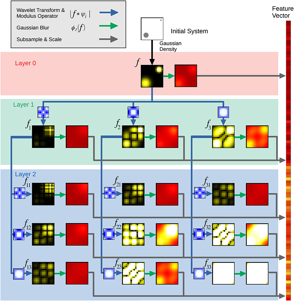
Figure 1. Schematic illustrating the scattering transform. The different layers are formed by systematic applications of the wavelet transform, modulus operator, Gaussian blur, and subsampling and scaling. Each of these different processes is represented by different colored arrows. The data is collected into a feature vector for the scattering transform machine learning.

In the first layer (0), a Gaussian filter ϕ_J0(f) at scale J₀ blurs the density f. The coefficients of the blurred density are subsampled, averaged, and stored as part of the ST representation. During subsampling, a discretized vector is sampled at a coarser resolution to form a smaller vector for the final representation.

To obtain the second layer (1), various wavelet transforms are applied to f; the convolutions f * ψ_{j1, 0} are computed at various length scales j₁ before calculating the modulus (absolute value) of each of these averaged coefficients as another part of the ST representation. This modulus operation introduces the nonlinearities mentioned earlier. After computing the modulus, we again blur using a Gaussian filter ϕ_J1(f) and subsample, this time at scale J₁ and store the resulting coefficients as part of the scattering representation.

To obtain the third layer (2) another wavelet transform is applied, yielding |f * ψ_{j1, 0}| * ψ_{j2, 0} for each length scale j₂. Each of these again has the modulus operator applied, is blurred, and is subsampled to produce coefficients as done in previous layers. Similar to other convolutional neural networks, this process could continue for many more layers. Of course, the ability to capture the relevant features will depend upon the relative scales of the atomic structures and the wavelets employed. Once the scales of the wavelets have been set, these features will not be affected by including more copies of a periodic structure, like those often present in GBs. In this respect, the scattering features are not dependent on increased system size.

The ST produces a 1 × N vector for each GB, where N is determined by the ST parameters (i.e., chiefly the number of convolutional layers, the number and scale of the wavelet functions, and the severity of the subsampling). In contrast to SOAP, the ST produces a single vector per GB and thus requires no additional statistical post-processing to produce the feature vector for the GB.

Given the availability of discrete convolutional neural network software that is optimized for both CPU and GPU architectures, it is worth noting why continuous convolutions are worth the extra implementation effort compared to using discrete convolutions. Convolutional neural networks in deep learning were developed to handle image learning tasks, which are inherently discrete due to pixels in images. Physical systems, like the atomistic view of GBs, have smooth transitions that are represented more naturally by spherical harmonics and continuous wavelet functions. While it is true that neural network architectures can approximate curved decision boundaries², continuous wavelets are a more natural choice because they lead to a sparser representation (Hirn et al., 2015, 2017; Eickenberg et al., 2017).

2.3. Grain Boundary Structures and Properties

The SOAP and the ST are both representations that provide a feature matrix that is convenient for machine learning of GB structures. In the present work, we learn on the Olmsted GB database, which is a collection of 388 computed Ni GBs created by Olmsted et al. (2009a) using the Foiles-Hoyt embedded atom method (EAM) potential (Foiles and Hoyt, 2006).

The GB structures were created following standard methods where a fairly comprehensive list of initial atomic configurations are each minimized to determine which of all the configurations represents the minimum energy structure of the GB (Olmsted et al., 2009a). Using these GB structures, a variety of properties can be measured or calculated from simulations; for this work, our interest is in energy, temperature-dependent mobility, and shear coupling of the 388 GBs.

The GB energy is defined as the excess energy relative to the bulk as a result of the irregular structure of the atoms in the GB (Tadmor and Miller, 2011). It is important to note that GB energy is normally defined as a static property of the system measured at T = 0 K, and all atomistic structures examined in the machine learning are the T = 0 K structures associated with this calculation. The GB energies for the Olmsted GB database are available in the supplemental materials of Olmsted et al. (2009a). Since the energies for this dataset were calculated using an EAM potential, learning energies serves merely as a benchmark to demonstrate whether a given descriptor captures any physically relevant information useful for machine learning.

Temperature-dependent mobility and shear coupled GB migration are two dynamic properties related to the behavior of a migrating GB. The mobility of a GB is defined as the proportionality factor relating how fast a GB will migrate when subjected to a given driving force (Gottstein and Shvindlerman, 2010). The temperature-dependent mobility has to do with how the mobility changes with temperature. In most cases, mobility is a thermally activated process, where the mobility increases with increasing temperature. However, in analyzing the temperature-dependent mobility of the GBs in the Olmsted database (Olmsted et al., 2009b) and Homer et al. (2014) noticed four broad categories of temperature-dependent mobility: (i) thermally activated, (ii) non-thermally activated, (iii) mixed modes, and (iv) immobile/unclassifiable. These categories correspond with whether the mobility follows an Arrhenius relationships with temperature (thermally activated), does not follow an Arrhenius relationship with temperature (non-thermally activated), shows some mixed mode combination of thermally activated and non-thermally activated, or is immobile or simply unclassifiable.

In addition, when GBs migrate, they can also exhibit a coupled shear motion, in which the motion of a GB normal to its surface couples with lateral motion of one of the two crystals (Cahn et al., 2006; Homer et al., 2013). GBs are then classified as either exhibiting shear coupling or not.

2.4. Machine Learning

The SOAP and ST structure characterizations of the 388 GBs in the Olmsted database are calculated using the methods described above. Parameters for these calculations are defined for the SOAP as the radial basis cutoff (n_max), angular basis (spherical harmonic) cutoff (l_max), and the radial cutoff (r_cut) which are set to 18, 18 and 5.0 respectively in the present work. For the ST the parameters are defined as the size of the density discretization grid (density=0.25), the number of convolutional layers as seen in Figure 1 (Layers=2, which also includes Layer 0), a parameter that defines a singular spherical harmonic angular function (SPH_L=4), the number of wavelets at different scales used at each layer (n_trans=16), and the number of angular augmentations in the azimuthal and polar angles (n_angle1=16, n_angle2=16). An angular augmentation is when the density function is duplicated and rotated to form a new density function, which is also fed through the scattering network. The vectors produced from the rotated density function are then concatenated to form the final ST vector. For example, with n_angle1 = 16 and n_angle2 = 16, we end up with 256 copies of the density function, each of which produces a scattering vector. These are then concatenated together to produce the final ST vector. This provides a level of rotational invariance since it is not explicit in the ST.

With both the SOAP and ST providing feature matrices, we are now able to apply a machine learning approach on the SOAP, ST, and combined SOAP+ST characterizations of the GBs. The combined SOAP+ST characterization feature vector is created by simply concatenating the SOAP and ST vectors together. Gradient boosted decision trees [as implemented in xgboost (Chen and Guestrin, 2016)] are used to analyze and predict the GB energy, temperature-dependent mobility, and shear coupling.

For the machine learning of the properties, it is important to note that GB energy is a continuous quantity, while temperature dependent mobility trend and shear coupling are classification properties. The mobility and shear coupling properties present an imbalanced class problem, where one class contains many more samples than the other classes. Consequently, the machine learning models favor this larger class to minimize error, but this degrades the ability of the model to generalize to new data. For example, imagine a binary classification problem where the training data has 99% in one class and only 1% of the other. The machine learning model will perform best by just predicting 100% of the first class. Thus to address this issue, we used the Synthetic Minority Over-sampling Technique (SMOTE), which is a standard approach used in imbalanced class machine learning problems (Han et al., 2005), as implemented in the imblearn package to oversample the minority classes. We can conceptualize SMOTE by imagining a line segment connecting each instance of the minority class to every other instance of that minority class. The algorithm then synthetically creates instances of the minority class randomly along these line segments and adds them to the data set, thus oversampling and balancing the number of samples in each class. This approach could present issues if any classes are not separable (e.g., the classes overlap), but even in these cases SMOTE is expected to improve learning over simply using the imbalanced classes.

In addition to using SMOTE to address the class imbalance, we also consider two different splits of the temperature-dependent mobility. In a 4 class split, we use the four categories as defined above (Homer et al., 2014). In a 3 class split, we essentially combined the non-thermally activated and mixed modes into a single class, such that the three classes are essentially, (i) thermally activated, (ii) mobile but not thermally activated, and (iii) immobile/unclassifiable. The original machine learning on this data by Rosenbrock et al. (2017) used this same 3 class split.

We trained each model with a 50–50 train-test split. While decision trees have many different tunable hyperparameters, only the number of estimators (the number of trees) was tuned, using a process called Early Stopping (Zhang et al., 2005) with 5-fold cross validation. An ensemble of decision trees is trained by adding trees in multiple fitting rounds, with each new tree's parameters optimized using a loss function. By limiting the number of fitting rounds, the model will only grow until the accuracy never improves for the specified number of rounds. Thus, the optimal number of estimators can be found to minimize the chance of over-fitting.

3. Results and Discussion

A summary of the machine learning results of GB energy, temperature-dependent mobility, and shear coupling by the SOAP, ST, and Combined SOAP+ST methods is found in Table 1. To provide a reference against which to judge the machine learning results, we define a baseline “Random” quantity, as implemented in the original SOAP formulation (Rosenbrock et al., 2017). For this “Random” column, energies are drawn from a normal distribution with the same mean and standard deviation as the training data and then compared to the actual values in the validation data. For the mobility and shear coupling classification, random selection of classes from the training data are picked and compared against the validation data.

TABLE 1

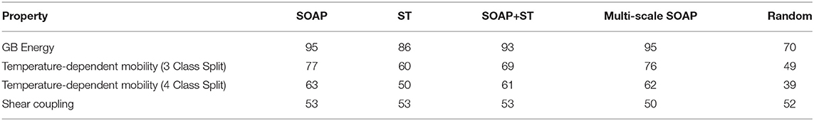
Table 1. Machine learning % accuracy of different properties by different techniques.

The ST results for energy and temperature-dependent mobility are statistically better than random and demonstrate that this new, universal representation is capable of learning certain GB structure-property relationships. However, it does not perform as well as the SOAP, and does not improve predictions even when it is combined with SOAP (SOAP+ST). Valid predictions are being made, but on different features of the GB atomic structure.

It is worth noting that the predictions of temperature-dependent mobility is worse for the 4 class split than the 3 class split. We attribute this to the reduced number of GBs in each class on which to learn and then make predictions, and which aggravates the imbalanced class problem. If our attribution is correct, this suggests how even a minor increase in data for each class (e.g., from 4 to 3 classes of the 388 GBs) can have a significant impact on the learning and prediction ability.

On its own, the ability to predict GB properties using machine learning has only limited benefits. For example, predicting the energy of the GBs here is merely an exercise. Computing energies from structures is not difficult, but predicting the mobility and shear coupling of a GB is and these properties have implications for material processing and deformation. Thus, we desire to use machine learning models to highlight new physical processes governing these properties. ST was introduced here because it targets different features of the GB atomic structure than SOAP. It follows then that each may highlight different physical processes that contribute to the same structure-property relationship, an assertion that would be born out by improvements to the machine learning accuracies.

A comparison of the learning rates is provided in Figure 2. In this figure it can be seen that the SOAP has better training and test accuracies than ST. Furthermore, according to the current slopes of the learning rates, there is no indication, at this point, that ST will perform better than SOAP. For now, one must conclude that ST learns different information about the GB structures, and this information is less helpful for accurate property prediction than the information provided by SOAP.

FIGURE 2

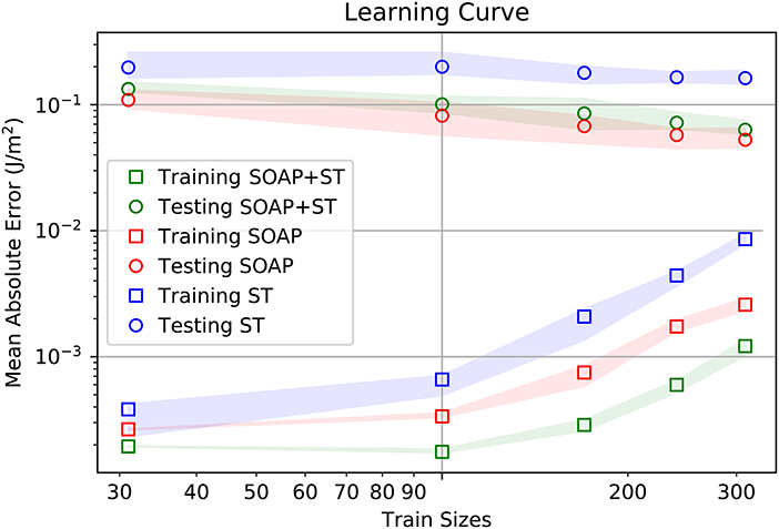
Figure 2. Learning rates for training and testing of GB energy for the averaged SOAP representation (SOAP), Scattering Transform (ST), and combined SOAP+ST descriptor. Mean absolute value for the energy across the GB database is about 1.09 J/m².

Interestingly, the SOAP+ST has the lowest training error, while having slightly worse test error than SOAP alone. This is indicative that the information provided by ST is useful in improving the training accuracy of the model. Unfortunately, the increase in error from SOAP alone to SOAP+ST indicates that the additional information provided by ST does not generalize to accurate property predictions on other GB structures. This would indicate that the SOAP+ST is suffering from over-fitting.

To understand and interpret these results, it is helpful to examine the characteristics of the SOAP and ST descriptors. While SOAP is formally complete in its rotational invariance (see Equation 4), the ST is formally complete in its translational invariance due to its convolution integral in Equation (6). In practice, the rotational invariance for ST is introduced by augmenting the representation with several discretely rotated copies of the data. Thus rotational invariance is only approximate for ST, whereas it is formally exact for SOAP. On the other hand, because ST uses multiple wavelets at different scales, it formally handles multi-scale translational invariance. Translational invariance for the SOAP representation originates in the use of local environments defined relative to a central atom, though the length-scale is limited by the cutoff radius of the SOAP descriptor.

The SOAP representation uses spherical harmonics to capture the angular information in the local environment density function. For this implementation of ST, we used periodic spherical harmonic wavelets to capture the periodicity of the GB structure in the dimensions of the boundary plane. It is likely that this choice of basis introduced some similarity in the features extracted by both SOAP and ST, but SOAP remains a local approach while ST operates at multiple scales.

One could also characterize multiple scales using SOAP by concatenating multiple SOAP vectors with varying cutoff and σ_atom parameters, as has been done in other works (Bartók et al., 2017; Willatt et al., 2018). At larger radial cutoffs, the surface area of the sphere for the local environment grows as $r_{\text{cutoff}}^2$, which introduces larger distances between atoms at the surface of the sphere. If the width of the Gaussian density (σ_atom) placed at each atom remains small, the angular resolution of the SOAP expansion cannot distinguish atom densities well. Thus, increasing the width of the Gaussian at each atom in proportion to the radial cutoff compensates for this geometrical effect so that more distant atoms are still resolved well. However, larger Gaussians placed at neighboring atoms close to the central atom cause structural information to be washed out. This necessitates including multiple SOAP vectors at different cutoffs and σ_atom values. To demonstrate the effectiveness of this approach, we compare the accuracy of this method with the others listed in Table 1. Here it can be seen that the multi-scale SOAP performs almost equal to standard SOAP, with values slightly worse for several properties. This also means that it performs better than ST and SOAP+ST.

While one could conclude from these results that ST does not provide sufficient improvement to the learning to justify its use, we believe there are some reasons to withhold judgment. There are three attributes to the ST that should be considered further. These are (i) data availability, (ii) interpretability, and (iii) overall utility as a structural descriptor.

First, concerning data availability, the ST uses layered convolutional neural networks, which generally provide high accuracy predictions in machine learning. It is worth noting that convolutional neural networks are frequently trained with tens of thousands or more datapoints. It is possible that more data may simply be required for the convolutional neural network used by ST to accurately learn GB properties.

One can increase the size of the GB dataset by constructing additional GB structures, which is time consuming and non-trivial. Or, one can increase the dataset by simulating existing GB structures at finite temperatures, where thermal fluctuations will lead to a large number of similar atomic configurations. We employ the latter approach in simulations of a Σ5 $(0\bar{1}3)/(0\bar{1}\bar{3})$, 〈100〉 symmetric tilt GB at 100 K over 10 ns and generate 1000 configurations, or snapshots, for that GB. If the ST is used to train a model on some configurations and test the model on the remaining, ST predicts with low mean absolute error. For example, with a single GB trained on 250 configurations and tested on the other 750 configurations, a mean absolute error of 0.002 J/m² is obtained. On the other hand SOAP trained on that same data results in a mean absolute error of 0.0015 J/m². Thus, with significantly more data ST improves significantly, though still not better than SOAP in this case.

The expanded MD dataset demonstrates that ST performs well with additional data. However, such datasets are moving toward the realm of “big data.” For example, if one desires to predict properties for any conceivable GB structure, significantly more data will be needed to train a general ST model.

The second attribute of ST that is worth discussing is the interpretability of the results and the ability to learn the underlying physics surrounding the machine learning predictions. By using the ST to provide the feature matrix, one can also perform an inverse scattering transform using relevance propagation to understand what aspects of the structure are influencing the learning. Specific details on the application of relevance propagation to ST is forthcoming (Nguyen, to be submitted). However, Figure 3 shows heatmaps generated using relevance propagation for the energy learning task. In Figure 3A we show a relevance propagation heatmap for learning of GB energy using a 50/50 split of the Olmsted database (i.e., the learning task reported in Table 1). Contrast that with the relevance propagation heatmap in Figure 3B where energy was learned from 500/500 split of the MD configurations noted above. In comparing the two images it is clear that Figure 3A highlights a seemingly random selection of atoms that are not consistent with the symmetry of the periodic structure of the GB. In Figure 3B, the well-known kite structure from the structural unit model is highlighted, despite the fact that the model had no knowledge of this structure a priori. Thus, the inverse ST relevance propagation heatmaps may allow one to identify the relevant features of the GB structure that correlate with the property of interest. The heatmaps in Figure 3 would be different for each property even though the structure of the GB might be the same. This could be crucial to the identification of the relevant features of the GB structure controlling different properties.

FIGURE 3

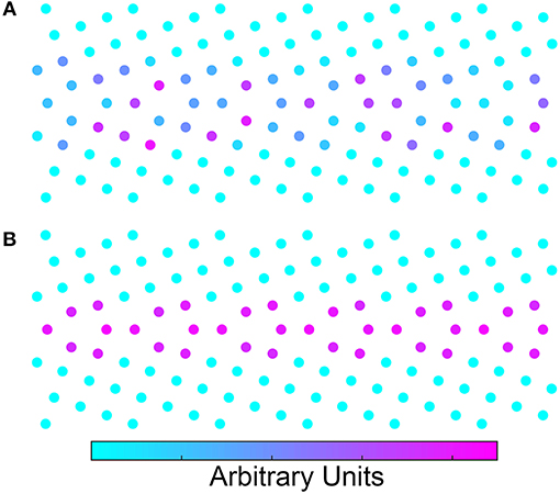
Figure 3. (A) Inverse scattering transform of the Σ5 $(0\bar{1}3)/(0\bar{1}\bar{3})$ GB. The model was trained using only half of the 388 GBs. (B) Inverse scattering transform of the same GB except that this model was trained using 500 configurations of the same GB. To obtain the configurations, a 10 nanosecond molecular dynamics simulation was performed at 100 K. Configurations were extracted every 10 picoseconds. Both models look down the [100] tilt axis of the crystals. The units for the inverse scattering transform are arbitrary.

Furthermore, while Rosenbrock et al. (2017) demonstrated that a derived form of SOAP, called the local environment representation, provides a way to interpret relevant GB structures, SOAP itself can be difficult to interpret. The multi-scale SOAP, which can provide longer range structural information, would be more difficult than SOAP by itself. Thus, while ST may not lead to the highest prediction values, its interpretability through the relevance propagation may render it a useful tool.

The overall utility as a structural descriptor is the third attribute of ST that is worth considering. To consider this we compare ST to a range of structural descriptors and their properties.

In Table 2 we summarize descriptors introduced for characterizing GBs, and from which machine learning models could be built. In addition to the metrics described in this work we also compare attributes against the structural unit model (SUM), dislocation arrays (DA), common neighbor analysis (CNA), polyhedral template matching (PTM), Voronoi cell topology (VCT), and the polyhedral unit model (PUM), all of which were mentioned in the introduction.

TABLE 2

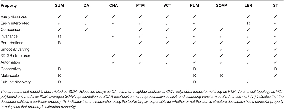
Table 2. Comparison of structural descriptors and their properties.

We judge each descriptor based on its usefulness across several metrics. The properties of interest are: Easily Visualized- one can convey the structures through visual means, Easily Interpreted–one can easily identify the relevant characteristics and differences between structures, Comparison- one can quantitatively compare the structures to one another, Invariance–the characterization is invariant to rotations, permutations, and/or translations, Perturbations–perturbations in the structure are captured as small changes in the metric, Smoothly Varying–the metric is continuous and varies smoothly for larger changes in structure, 3D GB Structures–the characterization works for quasi-2D and complex 3D GB structures, Automation–the characterization process can be automated, Connectivity–the technique characterizes how all the atoms in the GB are connected, Multi-scale–the technique characterizes both short- and long-range structural information, Subunit Discovery–the technique does not require a preset list of structures, it can discover them on its own.

While there are notable things about each descriptor and some of the entries in Table 2 are subjective, we will focus on a few properties of interest. In particular, we'll focus on a few of the properties not present in SOAP.

First, the ability to automate the description is an essential requirement to move GB science into the big data age. This property is shared by many. Second, is the ability to provide multi-scale characterization. Many techniques possess this ability if the researcher knows what they are doing, but ST is the only technique that possesses this inherently. Third and fourth are easily visualized and interpreted, which are two properties that are more subjective. Neither of these properties is a strength of SOAP³, but both could be a strengths of ST as evidenced by the heatmaps in Figure 3. Sixth is connectivity. ST does not possess this outright as one might consider in the structural unit model or in a graph description. However, it should be noted that while Figure 3 colors each of the atoms by their relevance in predicting energy, the continuous nature of ST and the inverse ST means that relevance scores are available continuously throughout the space; one could produce high resolution heatmaps. Having a detailed 3D “importance density” for a grain boundary would allow connectivity values between a graph of nearest-neighbor atoms to be quantified (for example by integrating the density along the path connecting the atoms). These edge weights in the connectivity graph could be thresholded to provide alternate views of connectivity. This definition of connectivity is somewhat different from the traditional definition. The heatmaps also change based on the property of interest rather than being static. That in turn, may be more useful for discovering the physical underpinnings on structure-property relationships. This approach might also allow one to fulfill the final property of subunit discovery. Again, this isn't currently present in ST, but one could imagine how the inverse ST heatmaps might enable this property.

Considering these three attributes of ST, there is reason to believe that the ST, or something very similar, might become an important descriptor for GB data science. However, given the evidence presented here, one must proceed with caution, and consider other ways to achieve the same goals of encoding the most useful information about GB structures for property prediction and discovery of the underlying physics.

4. Conclusion

The success of machine learning in GB data science will largely be guided by the development of tools that capture the physical essence of GB structure-property relationships. These tools must be automated and universally applicable to large and complex GB structures. Since the machine learning is merely a stepping stone to discovery of the underlying physics, these tools should also satisfy certain mathematical constraints related to invariances and smoothness.

We introduced a new descriptor, the Scattering Transform (ST) (Bownik, 1997; Benedetto and Pfander, 1998; Pfander and Benedetto, 2002; Beńıtez et al., 2010; Goh and Lee, 2010; Goh et al., 2011; Lanusse et al., 2012; Mallat, 2012), based on continuous, multi-scale wavelet transforms interleaved with modulus nonlinearities. We showed that this descriptor can effectively learn GB structure-property relationships for energy and does reasonably well for temperature-dependent mobility. It should be noted that the SOAP descriptor surpassed the ST in prediction accuracy and remains the optimal descriptor for the properties and structures compared here.

However, we also demonstrated that despite its inability to achieve the same accuracy predictions as SOAP, ST has complimentary features that may make it a useful descriptor of GB structure. First off, the ST information content is different than and complementary to that of the SOAP descriptor. The ST has the ability to encode multi-scale structural information and be visualized using an inverse ST that generates a heatmap. Importantly, the inverse ST provides evidence of the prevailing wisdom that multi-level convolutional networks require large amounts of data in order to truly learn the physics underlying structure-property relationships. This helps contextualize the performance of ST relative to the averaged SOAP representation and other SOAP-based representations. It also motivates the building of much larger GB databases.

The ST has the potential to be a powerful tool in understanding GB structure-property relationships. As we continue to push the limits of our understanding in GB structure-property relationships it will be most valuable to (i) focus on building larger databases of GB structure-property mappings, which currently represents the greatest limitation, and (ii) continue to introduce new descriptors that satisfy as many of the desirable characteristics as possible.

Data Availability

The datasets for this manuscript are not publicly available. Requests to access the datasets should be directed to Stephen Foiles, foiles@sandia.gov.

Author Contributions

CR, AN, EH, and GH all conceived the idea for this work. AN wrote the code for the scattering transform. DH performed all the calculations. All were involved in writing the manuscript.

Funding

DH, CR, AN, and GH are supported under ONR (MURI N00014-13-1-0635). EH is supported by the U.S. Department of Energy, Office of Science, Basic Energy Sciences under Award #DE-SC0016441.

Conflict of Interest Statement

The authors declare that the research was conducted in the absence of any commercial or financial relationships that could be construed as a potential conflict of interest.

Footnotes

1. ^This is available from the Python Package Index using pip install pycsoap.

2. ^The interactive 2D playground at https://playground.tensorflow.org demonstrates this nicely.

3. ^SOAP can lends itself to interpretation by either (i) optimizing a reference structure by minimizing the kernel metric distance, much like the local environment representation, or (ii) applying relevance propagation to the SOAP vector. However, the first approach provides only a local analog and the second approach suffers information loss due to the angular integral. Thus, while certainly useful, the inverse SOAP operations do not have the same global resolution as an inverse scattering transform.

References

Baldock, R. J. N., Pártay, L. B., Bartók, A. P., Payne, M. C., and Csányi, G. (2016). Determining pressure-temperature phase diagrams of materials. Phys. Rev. B 93:174108. doi: 10.1103/PhysRevB.93.174108

CrossRef Full Text | Google Scholar

Balluffi, R. W., and Bristowe, P. D. (1984). On the structural unit/grain boundary dislocation model for grain boundary structure. Surface Sci. 144, 28–43.

Google Scholar

Banadaki, A. D., and Patala, S. (2017). A three-dimensional polyhedral unit model for grain boundary structure in fcc metals. NPJ Comput. Mater. 3:13. doi: 10.1038/s41524-017-0016-0

CrossRef Full Text | Google Scholar

Bartók, A. P., De, S., Poelking, C., Bernstein, N., Kermode, J. R., Csányi, G., et al. (2017). Machine learning unifies the modeling of materials and molecules. Sci. Adv. 3, e1701816–B871. doi: 10.1126/sciadv.1701816

PubMed Abstract | CrossRef Full Text | Google Scholar

Bartók, A. P., Kondor, R., and Csányi, G. (2013). On representing chemical environments. Phys. Rev. B 87:184115. doi: 10.1103/PhysRevB.87.184115

CrossRef Full Text | Google Scholar

Bartók, A. P., Payne, M. C., Kondor, R., and Csányi, G. (2010). Gaussian approximation potentials: the accuracy of quantum mechanics, without the electrons. Phys. Rev. Lett. 104:136403. doi: 10.1007/978-3-642-14067-9

PubMed Abstract | CrossRef Full Text | Google Scholar

Benedetto, J. J., and Pfander, G. E. (1998). “Wavelet periodicity detection algorithms,” in Wavelet Applications in Signal and Imaging Processing VI, eds A. F. Laine, M. A. Unser, and A. Aldroubi (San Diego, CA: International Society for Optics and Photonics), 48–56.

Google Scholar

Benítez, R., Bolós, V. J., and Ramírez, M. E. (2010). A wavelet-based tool for studying non-periodicity. Comput. Math. Appl. 60, 634–641. doi: 10.1016/j.camwa.2010.05.010

CrossRef Full Text | Google Scholar

Bishop, G. H., and Chalmers, B. (1968). A coincidence - ledge - dislocation description of grain boundaries. Scrip. Metal. Mater. 2, 133–140.

Google Scholar

Bownik, M. (1997). Tight frames of multidimensional wavelets. J. Four. Anal. Appl. 3, 525–542.

Google Scholar

Cahn, J. W., Mishin, Y., and Suzuki, A. (2006). Coupling grain boundary motion to shear deformation. Acta Mater. 54, 4953–4975. doi: 10.1016/j.actamat.2006.08.004

CrossRef Full Text | Google Scholar

Caro, M. A., Aarva, A., Deringer, V. L., Csányi, G., and Laurila, T. (2018). Reactivity of amorphous carbon surfaces: rationalizing the role of structural motifs in functionalization using machine learning. Chem. Mater. 30, 7446–7455. doi: 10.1021/acs.chemmater.8b03353

PubMed Abstract | CrossRef Full Text | Google Scholar

Chen, T., and Guestrin, C. (2016). “Xgboost: a scalable tree boosting system,” in Proceedings of the 22Nd ACM SIGKDD International Conference on Knowledge Discovery and Data Mining, KDD '16 (New York, NY: ACM), 785–794.

Google Scholar

Cisneros, G. A., Wikfeldt, K. T., Ojamäe, L., Lu, J., Xu, Y., Torabifard, H., et al. (2016). Modeling molecular interactions in water: From pairwise to many-body potential energy functions. Chem. Rev. 116, 7501–7528. doi: 10.1021/acs.chemrev.5b00644

PubMed Abstract | CrossRef Full Text | Google Scholar

De, S., Bartók, A. P., Csányi, G., and Ceriotti, M. (2016). Comparing molecules and solids across structural and alchemical space. Phys. Chem. Chem. Phys. 18, 13754–13769. doi: 10.1039/C6CP00415F

PubMed Abstract | CrossRef Full Text | Google Scholar

Dragoni, D., Daff, T. D., Csányi, G., and Marzari, N. (2018). Achieving dft accuracy with a machine-learning interatomic potential: thermomechanics and defects in bcc ferromagnetic iron. Phys. Rev. Mater. 2:013808. doi: 10.1103/PhysRevMaterials.2.013808

CrossRef Full Text | Google Scholar

Eickenberg, M., Exarchakis, G., Hirn, M., and Mallat, S. (2017). “Solid harmonic wavelet scattering: predicting quantum molecular energy from invariant descriptors of 3d electronic densities,” in Advances in Neural Information Processing Systems 30, eds I. Guyon, U. V. Luxburg, S. Bengio, H. Wallach, R. Fergus, S. Vishwanathan et al. (Long Beach, CA: Curran Associates, Inc.), 6540–6549.

Google Scholar

Foiles, S. M., and Hoyt, J. (2006). Computation of grain boundary stiffness and mobility from boundary fluctuations. Acta Mater. 54, 3351–3357. doi: 10.1016/j.actamat.2006.03.037

CrossRef Full Text | Google Scholar

Frank, F. C. (1988). Orientation mapping. Metall. Trans. A 19, 403–408.

Google Scholar

Frost, H. J., Spaepen, F., and Ashby, M. F. (1982). A second report on tilt boundaries in hard sphere F.C.C. crystals. Scrip. Metall. Mater. 16, 1165–1170.

Google Scholar

Goh, S. S., Han, B., and Shen, Z. (2011). Tight periodic wavelet frames and approximation orders. Appl. Comput. Harmon. Analy. 31, 228–248. doi: 10.1016/j.acha.2010.12.001

CrossRef Full Text | Google Scholar

Goh, S. S., and Lee, S. L. (2010). “Wavelets, multiwavelets and wavelet frames for periodic functions,” Proceedings of the 6th IMT-GT Conference on Mathematics, Statistics and its Applications ICMSA, Kuala Lumpur.

Google Scholar

Gottstein, G., and Shvindlerman, L. S. (2010). Grain Boundary Migration in Metals. Boca Raton: CRC Press.

Google Scholar

Han, H., Wang, W.-Y., and Mao, B.-H. (2005). “Borderline-smote: a new over-sampling method in imbalanced data sets learning,” in Proceedings of the 2005 International Conference on Advances in Intelligent Computing - Volume Part I, ICIC'05 (Berlin; Heidelberg: Springer-Verlag), 878–887.

Google Scholar

Han, J., Vitek, V., and Srolovitz, D. J. (2016). Grain-boundary metastability and its statistical properties. Acta Mater. 104, 259–273. doi: 10.1016/j.actamat.2015.11.035

CrossRef Full Text | Google Scholar

Han, J., Vitek, V., and Srolovitz, D. J. (2017). The grain-boundary structural unit model redux. Acta Mater. 133, 186–199. doi: 10.1016/j.actamat.2017.05.002

CrossRef Full Text | Google Scholar

Hirn, M., Mallat, S., and Poilvert, N. (2017). Wavelet scattering regression of quantum chemical energies. Multiscale Model. Simulat. 15, 827–863. doi: 10.1137/16M1075454

CrossRef Full Text | Google Scholar

Hirn, M., Poilvert, N., and Mallat, S. (2015). Quantum energy regression using scattering transforms. arXiv [Preprint] arXiv:1502.02077.

Google Scholar

Homer, E. R., Foiles, S. M., Holm, E. A., and Olmsted, D. L. (2013). Phenomenology of shear-coupled grain boundary motion in symmetric tilt and general grain boundaries. Acta Mater. 61, 1048–1060. doi: 10.1016/j.actamat.2012.10.005

CrossRef Full Text | Google Scholar

Homer, E. R., Holm, E. A., Foiles, S. M., and Olmsted, D. L. (2014). Trends in grain boundary mobility: survey of motion mechanisms. J. Miner. Metals Mater. Soc. 66, 114–120. doi: 10.1007/s11837-013-0801-2

CrossRef Full Text | Google Scholar

Honeycutt, J. D., and Andersen, H. C. (1987). Molecular dynamics study of melting and freezing of small Lennard-Jones clusters. J. Phys. Chem. 91, 4950–4963.

Google Scholar

John, S. T., and Csányi, G. (2017). Many-body coarse-grained interactions using gaussian approximation potentials. J. Phys. Chem. B 121, 10934–10949. doi: 10.1021/acs.jpcb.7b09636

PubMed Abstract | CrossRef Full Text | Google Scholar

Lanusse, F., Rassat, A., and Starck, J.-L. (2012). Spherical 3d isotropic wavelets. Astron. Astrophys. 540:A92. doi: 10.1051/0004-6361/201118568

CrossRef Full Text | Google Scholar

Larsen, P. M., Schmidt, S., and Schiøtz, J. (2016). Robust structural identification via polyhedral template matching. Model. Simulat. Mater. Sci. Eng. 24:055007. doi: 10.1088/0965-0393/24/5/055007

CrossRef Full Text | Google Scholar

Lazar, E. A. (2018). VoroTop: voronoi cell topology visualization and analysis toolkit. Model. Simulat. Mater. Sci. Eng. 26:015011. doi: 10.1088/1361-651X/aa9a01

CrossRef Full Text | Google Scholar

Mallat, S. (2012). Group invariant scattering. Comm. Pure Appl. Math. 65, 1331–1398. doi: 10.1002/cpa.21413

CrossRef Full Text | Google Scholar

Maresca, F., Dragoni, D., Csányi, G., Marzari, N., and Curtin, W. A. (2018). Screw dislocation structure and mobility in body centered cubic Fe predicted by a Gaussian Approximation Potential. NPJ Comput. Mater. 4:69. doi: 10.1038/s41524-018-0125-4

CrossRef Full Text | Google Scholar

Medlin, D. L., Foiles, S. M., and Cohen, D. (2001). A dislocation-based description of grain boundary dissociation: application to a 90 110 tilt boundary in gold. Acta Mater 49, 3689–3697. doi: 10.1016/S1359-6454(01)00284-1

CrossRef Full Text | Google Scholar

Mocanu, F. C., Konstantinou, K., Lee, T. H., Bernstein, N., Deringer, V. L., Csányi, G., et al. (2018). Modeling the phase-change memory material, ge2sb2te5, with a machine-learned interatomic potential. J. Phys. Chem. B 122, 8998–9006. doi: 10.1021/acs.jpcb.8b06476

PubMed Abstract | CrossRef Full Text | Google Scholar

Olmsted, D. L., Foiles, S. M., and Holm, E. A. (2009a). Survey of computed grain boundary properties in face-centered cubic metals: I. Grain boundary energy. Acta Mater. 57, 3694–3703. doi: 10.1016/j.actamat.2009.04.007

CrossRef Full Text | Google Scholar

Olmsted, D. L., Holm, E. A., and Foiles, S. M. (2009b). Survey of computed grain boundary properties in face-centered cubic metals-II: grain boundary mobility. Acta Mater. 57, 3704–3713. doi: 10.1016/j.actamat.2009.04.015

CrossRef Full Text | Google Scholar

Patala, S., Mason, J. K., and Schuh, C. A. (2012). Improved representations of misorientation information for grain boundary science and engineering. Progress Mater, Sci. 57, 1383–1425. doi: 10.1016/j.pmatsci.2012.04.002

CrossRef Full Text | Google Scholar

Patala, S., and Schuh, C. A. (2013). Symmetries in the representation of grain boundary-plane distributions. Philos. Magaz. 93, 524–573. doi: 10.1080/14786435.2012.722700

CrossRef Full Text | Google Scholar

Pfander, G. E., and Benedetto, J. J. (2002). Periodic wavelet transforms and periodicity detection. SIAM J. Appl. Math. 62, 1329–1368. doi: 10.1137/S0036139900379638

CrossRef Full Text | Google Scholar

Priedeman, J. L., Rosenbrock, C. W., Johnson, O. K., and Homer, E. R. (2018). Quantifying and connecting atomic and crystallographic grain boundary structure using local environment representation and dimensionality reduction techniques. Acta Mater. 161, 431–443. doi: 10.1016/j.actamat.2018.09.011

CrossRef Full Text | Google Scholar

Randle, V. (2010). Grain boundary engineering: an overview after 25 years. Mater. Sci. Tech. 26, 253–261. doi: 10.1179/026708309X12601952777747

CrossRef Full Text | Google Scholar

Read, W. T., and Shockley, W. (1950). Dislocation models of crystal grain boundaries. Phys. Rev. 78, 275–289.

Google Scholar

Rittner, J. D., and Seidman, D. N. (1996). 110 symmetric tilt grain-boundary structures in fcc metals with low stacking-fault energies. Phys. Rev. B 54, 6999–7015.

Google Scholar

Rosenbrock, C. W., Homer, E. R., Csányi, G., and Hart, G. L. W. (2017). Discovering the building blocks of atomic systems using machine learning: application to grain boundaries. NPJ Comput. Mater. 3:29. doi: 10.1038/s41524-017-0027-x

CrossRef Full Text | Google Scholar

Rosenbrock, C. W., Priedeman, J. L., Hart, G. L., and Homer, E. R. (2018). Structural characterization of grain boundaries and machine learning of grain boundary energy and mobility. arXiv arXiv:1808.05292.

Google Scholar

Sosso, G. C., Deringer, V. L., Elliott, S. R., and Csányi, G. (2018). Understanding the thermal properties of amorphous solids using machine-learning-based interatomic potentials. Mol. Simulat. 44, 866–880. doi: 10.1080/08927022.2018.1447107

CrossRef Full Text | Google Scholar

Spearot, D. E. (2008). Evolution of the E structural unit during uniaxial and constrained tensile deformation. Acta Mater. 35, 81–88. doi: 10.1016/j.mechrescom.2007.09.002

CrossRef Full Text | Google Scholar

Sutton, A. P., and Vitek, V. (1983). On the structure of tilt grain-boundaries in cubic metals. 1. symmetrical tilt boundaries. Philos. Trans. R. Soc. Math. Phys. Eng. Sci. 309, 1–36.

Google Scholar

Szlachta, W. J., Bartók, A. P., and Csányi, G. (2014). Accuracy and transferability of Gaussian approximation potential models for tungsten. Phys. Rev. B 90:104108. doi: 10.1103/PhysRevB.90.104108

CrossRef Full Text | Google Scholar

Tadmor, E. B., and Miller, R. E. (2011). Modeling Materials: Continuum, Atomistic and Multiscale Techniques. Cambridge: Cambridge University Press.

Google Scholar

Tschopp, M. A., and McDowell, D. L. (2007). Structural unit and faceting description of Sigma 3 asymmetric tilt grain boundaries. J. Mater. Sci. 42, 7806–7811. doi: 10.1007/s10853-007-1626-6

CrossRef Full Text | Google Scholar

Watanabe, T., Tsurekawa, S., Zhao, X., and Zuo, L. (2009). “The coming of grain boundary engineering in the 21st Century,” in Microstructure and Texture in Steels, eds A. Haldar, S. Suwas, and D. Bhattacharjee (London: Springer London), 43–82.

Willatt, M. J., Musil, F., and Ceriotti, M. (2018). Feature optimization for atomistic machine learning yields a data-driven construction of the periodic table of the elements. Phys. Chem. Chem. Phys. 20, 29661–29668. doi: 10.1039/C8CP05921G

PubMed Abstract | CrossRef Full Text | Google Scholar

Wolf, D. (1989). A read-shockley model for high-angle grain boundaries. Scrip. Metal. Mater. 23, 1713–1718. doi: 10.1016/0036-9748(89)90348-7

CrossRef Full Text | Google Scholar

Zhang, T.Yu, B., et al. (2005). Boosting with early stopping: convergence and consistency. Ann. Stat. 33, 1538–1579. doi: 10.1214/009053605000000255

CrossRef Full Text | Google Scholar