Adapting Artificial Intelligence to Improve In Situ Concrete Compressive Strength Estimations in Rebound Hammer Tests

Introduction

Concrete is a man-made composite material, consisting mainly of aggregate, water, and cement. Because it is relatively cheap and provides high compressive strength, concrete is one of the most commonly used materials in the construction industry. It is extensively used in buildings, bridges, roads, and many other structures. To ensure the safety of the structures, the quality of the concrete material, especially the concrete strength, is of great concern to the construction industry. One of the most popular ways to assess the performance of concrete is to measure its compressive strength. Compressive strength is one of the most important criteria used to examine whether a given concrete mixture will fulfill its design requirements. Compressive strength is typically measured by breaking cylinder concrete samples in a compressor machine. These specimens are randomly sampled from different ready-mixed concrete batches delivered to the construction site. Nevertheless, for existing structures, it is necessary to drill core samples in order to obtain concrete compressive strength in the field. Taking core samples causes certain damage to existing structures, and sometimes, it is not feasible to take core samples (for example, when you cannot obtain the owner’s consent). Under such circumstances, alternative testing methods, such as nondestructive tests, are desirable for assessing concrete compressive strength. Among the nondestructive concrete compressive strength tests, rebound hammer (RH) and ultrasonic pulse velocity (UPV) tests are commonly seen in the industry. The major benefits of RH and UPV tests are their abilities to examine the condition of a concrete structure without causing damage (Shariati et al., 2011).

In the RH test, a spring-loaded steel hammer is pushed against the surface of the concrete. When released, the hammer impacts the concrete with a predetermined amount of energy. The hardness of the concrete affects the extent of the elastic mass rebound. This rebound distance is measured and used to estimate the concrete strength (ASTM C805 / C805M – 18, 2020). In the UPV test, first, the propagation velocity of longitudinal stress wave pulses through concrete is measured. Then, the compressive strength of the concrete is estimated using the measured UPV. The UPV test is conducted by transmitting ultrasonic pulses through the test specimen, and then, the time taken by the pulse to pass through the concrete is measured. Higher velocities indicate good quality and continuity of the material, and lower velocities may indicate cracks or voids in the concrete (ASTM C597 – 16, 2020). Compared to other nondestructive methods, RH tests are cheaper (in terms of test equipment), faster, and easier to conduct (Hamidian et al., 2012). In addition, RH tests are adopted in the American Society for Testing and Materials (ASTM 805) (ASTM C597 – 16, 2020) and Chinese National Standards (CNS 10732) as an alternative way to assess concrete compressive strength. Therefore, this research utilizes RH tests to estimate concrete compressive strength.

Typically, the rebound distance measured is used to estimate concrete compressive strength either using the conversion table or equations provided by the manufacturer. Nevertheless, despite its convenience, compressive strength estimations from RH tests are not very accurate, and an average of more than 20% mean absolute percentage error (MAPE) is reported (Huang et al., 2011). In light of this, this research attempts to further examine the relationship between RH measurements and actual compressive strength.

Previous research has attempted different approaches to investigate the relationship between RH measurements and actual compressive strength. To achieve this goal, many researchers adopt linear and nonlinear statistical regressions to improve the concrete compressive strength estimation in the RH test (Hajjeh, 2012; Rojas-Henao et al., 2012; El Mir and Nehme, 2017; Xu and Li, 2018; Kocáb et al., 2019). In addition, some researchers have successfully adopted nontraditional statistical methods, such as artificial neural networks (ANNs), to improve concrete compressive strength estimations in RH tests (Yılmaz and Yuksek, 2008; Iphar, 2012; Asteris and Mokos, 2019). Nevertheless, most research uses new cube or cylinder samples produced in the laboratory. As a result, there might be some limitations when applying these research findings to in situ RH tests. In light of this, this research intends to investigate the relationships between RH measures and actual compressive strength for existing structures. In situ RH tests and core sampling are conducted on a large residential complex building. Both traditional (linear/nonliner regression) and nontraditional (artificial intelligence or AI) statistical analyses are conducted to develop concrete compressive strength prediction models. The research results show that, by introducing the AI methods into the RH tests, concrete compressive strength estimations can be improved for in situ test objects. It should be noted that the emphasis of this research is on examining the relationships between in situ RH measurements and concrete strength; therefore, the nature of the RH test itself is not discussed in this research.

Literature Review

By adopting AI methods, this research intends to investigate the relationships between in situ RH test measurements and actual concrete compressive strengths. First, previous research related to RH tests and concrete compressive strength estimation are reviewed. Then, literature related to AI methods are reviewed.

Rebound Hammer Test

When destructive test measures are not feasible, nondestructive testing methods have been adopted as an alternative to examine the properties of construction materials. Over the years, successful results have been obtained by researchers using nondestructive methods to estimate material properties (Kumar et al., 2019). For concrete material, the RH test is often chosen as an alternative nondestructive testing method to estimate compressive strength. RH test standards have been established in different countries and regions, such as ASTM 805 in the United States (ASTM C805 / C805M – 18, 2020), BS 1881: part 202 in the United Kingdom (British Standards Institution (BSI), 1986), EN 12504-2 in Europe (European Normalization Committee (En), 2012), and CNS 10732 in Taiwan The National Standards of the Republic of China, 1986. The RH test is easy to conduct, and the test results can be obtained almost instantly. RH measurements can be used to estimate concrete compressive strength either using a conversion table or a conversion equation provided by the instrument manufacturer. However, these concrete compressive strength estimations are not very accurate when using RH test measurements (Huang et al., 2011). Some researchers have attempted to improve concrete compressive strength estimations by introducing factors other than RH value, such as water:cement ratio, age, and types of admixture (Atoyebi et al., 2019). Others have attempted different prediction methods to better correlate the RH value with actual compressive strength. Among them, traditional statistical regressions are the most popular methods adopted by the researchers (Hajjeh, 2012; Rojas-Henao et al., 2012; El Mir and Nehme, 2017; Xu and Li, 2018; Kocáb et al., 2019). In recent years, nontraditional statistical regression methods, such as ANNs, are reported to have better compressive strength estimations when compared to traditional regression methods (Yılmaz and Yuksek, 2008; Iphar, 2012; Asteris and Mokos, 2020). In addition to traditional regression methods and ANNs, this research also adopts alternative AI methods, support vector regression, and adaptive network-based fuzzy inference systems (ANFIS) to develop concrete compressive prediction models. These methods are introduced in the next section.

Artificial Intelligence Methods

Some previous RH estimation research adopts traditional statistical methods to correlate RH measurements and concrete compressive strength. However, the results have not been satisfactory so far (Qasrawi, 2000; Szilágyi et al., 2011; Brencich et al., 2013; Breysse and Martínez-Fernández, 2014). This research attempts to use AI methods to investigate the relationship between RH measurements and concrete compressive strength. As an application of AI, machine learning algorithms use sample data to develop (or train) mathematical models. Learning from sample data allows the model to make predictions without being explicitly programmed (Bishop, 2006). For this research, RH experiments are conducted to obtain sample data for machine learning prediction models. Among the various machine learning techniques for regression, ANNs, support vector machines (SVMs), and ANFIS are chosen to develop the prediction models. For this research, these techniques are chosen because ANNs, SVMs, and ANFIS are reported to have been successfully applied in many different areas, such as finance, engineering, medicine, and manufacturing. The model prediction results from these AI techniques also outperformed traditional statistical regression methods (Shirsath and Singh, 2010; Balabin and Lomakina, 2011; Yilmaz and Kaynar, 2011; Rezaeianzadeh et al., 2014).

Based on the literature, this research adapts AI regression methods to improve concrete compressive strength estimation for in situ RH tests. The RH test and AI regression methods are briefly introduced in the next section.

Methodology

RH tests are popular nondestructive tests to measure the surface hardness and penetration resistance of concrete. RH test measurements can be related to the elastic properties or strength of the test object. In the RH tests, the hammer is first pressed against the concrete surface (small, nonstructural beams in this research). Next, the spring-loaded hammer mass strikes with a defined energy, and then the rebound is measured. The rebound value measured is known as the rebound number. By referring to the conversion table or equation provided by the manufacturer, the concrete compressive strength can then be estimated using the rebound number. For digital RH, the compressive strength can be automatically calculated (Information on, 2012). The RH gives an indication of the test object’s surface hardness. When using RH to examine concrete compressive strength, a lower rebound value is obtained for low strength and stiffness concrete due to more energy absorption (Brencich et al., 2013).

For this research, the research team first conducted RH tests on nonstructural beams in the basement of a large residential complex. After the RH tests, core samples were carefully drilled and then tested in the laboratory to obtain the actual compressive strength. Due to the destructive nature of the core drilling process, in situ RH test data are difficult to collect. In order to get more reliable concrete strength estimations, data from a total of 100 samples are collected. A digital RH (Silver Schmidt Type N-PC) is used for this research as shown in Figure 1. The digital hammer offers intuitive, menu-guided operation; electronic data processing; automatic correction for testing positions; and test data storage (Information on, 2012). This instrument is chosen because its accuracy and repeatability are improved compared to traditional concrete test hammers. The collected data are then used to develop and validate the AI regression models.

FIGURE 1

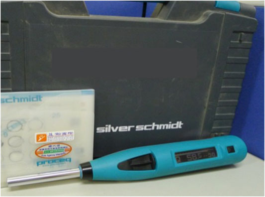
FIGURE 1. Silver schmidt type N-PC rebound hammer.

ANNs are machine learning methods that are inspired by the biological neural systems in the brain. An ANN consists of interconnected nodes (artificial neurons), and these nodes can receive, process, and transmit signals to artificial neurons connected to them. Each artificial neuron has weighted inputs, one transfer function, and one output. Although a single neuron can perform certain simple tasks, the real computation power comes from the interconnecting neurons. Typically, these interconnected neurons are aggregated into the input layer, the hidden layer(s), and the output layer. Signals are received by the input layer and then transmitted through the hidden layer(s) and output layer. Such systems are able to learn from examples without being programmed with task-specific rules (Zupan and Gasteiger, 1991; Gurney, 2014). A typical three-layer neural network is shown in Figure 2 with one input layer, one hidden layer, and one output layer.

FIGURE 2

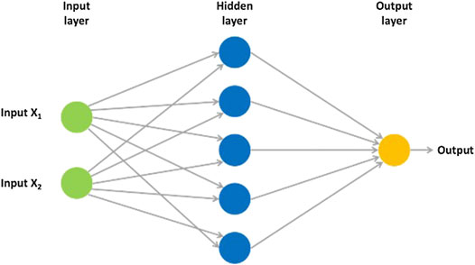
FIGURE 2. Three-layer ANNs.

In the hidden layer, the neurons receive activation signals from the neurons in the input layer. The activation signal entering each neuron is the weighted sum of all the signals from the input layer. This weighted sum of all signals (also known as activation signal) is shown in Eq. 1. In Eq. 1, x_j is the activation signal that neuron j in the hidden layer receives; I_i is ith neuron in the input layer, and W_ij is the weight of the connection between neuron j in the hidden layer and the input layer neuron I_i. After receiving the activation signals, the neuron generates an output through a predetermined activation function. One of the most common activation functions is the sigmoid function, illustrated in Eq. 2. In Eq. 2, x_j is the input for neuron j in the hidden layer and h_j is the output of neuron j. Sigmoid functions transform input values into output values between 0 and 1.

$x_j={\displaystyle \sum _i{I}_i{W}_{ij}}(1)$

$h_j=f\left(x_j\right)=\frac{1}{1+e^{-x_j}}(2)$

$y_k={\displaystyle \sum _j{h}_j{W}_{jk}}(3)$

The outputs of the hidden layer neurons are then transmitted to the output layer. As shown in Eq. 3, h_j is the output of neuron j and W_jk is the weight of the connection between neurons j and k. y_k is the activation signal received by the output layer neuron k, the weighted sum of inputs to the output layer neuron k. In the output layer, the activation function transforms the received activation signals and generates the outputs of the neural networks. As illustrated in Eq. 4, o_k is the output of the neural network model after sigmoid function transformation. For supervised neural networks, the model error, E(W), is then calculated by comparing the desired (or actual) value d_k and the model output o_k as calculated in Eq. 5.

$o_k=f\left(y_k\right)=\frac{1}{1+e^{-y_k}}(4)$

$E\left(W\right)=\frac{1}{2}{\displaystyle \sum _k{\left(d_k-o_k\right)}^2}(5)$

In neural network model development, the error function, E(W), is minimized to find the best fit model. One of the most popular techniques to minimize he error is the back-propagation (BP) algorithm. In the BP algorithm, the errors obtained at the output layers are propagated backward to the hidden layer and then to the input layer. During the BP process, the connecting weights between all the neurons in the networks are updated. With the updated weights, the network output is recalculated. The error obtained from the updated neural network is back-propagated to update the weights again. This process is repeated to minimize the error until the best fit model is found.

ANNs have been successfully applied in many research fields to make predictions. Some researchers have successfully adapted ANNs to predict concrete compressive strength using input variables such as age, Portland cement, water, sand, crushed stone, high range water-reducing agent, and fly ash (Topçu and Sarıdemir, 2008). This research also utilizes ANNs to develop the concrete strength prediction model.

SVMs, first purposed by Vapnik (2013), are supervised machine learning methods based on statistical learning theory. As shown in Figure 3, SVMs first conduct nonlinear mapping of sample data into the higher dimensional feature space, and then the sample data can be classified using a linear model. The Φ indicates the transformation function for the nonlinear mapping.

FIGURE 3

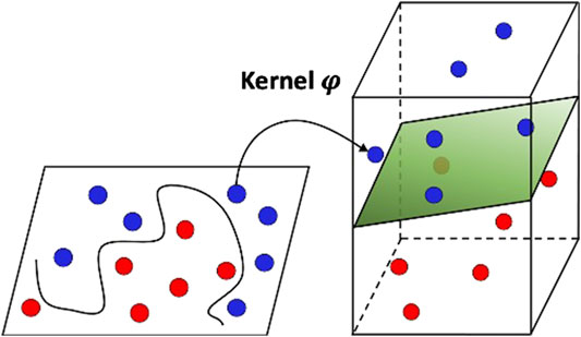
FIGURE 3. SVM higher dimension mapping.

SVMs were first developed for classification; Drucker et al. further proposed using the concepts for regression (Drucker et al., 1997), also known as support vector regression. The support vector regression concepts are briefly described below (Smola and Schölkopf, 2004).

For a given data set, $D={\left\{(x_i,d_i)\right\}}_i^n$, x_i is the input vector, d_i is the desired (target) value, and n is the size of the data set. With the nonlinear mapping (Φ) of the input vector, the nonlinear regression in the lower dimensional space can then be represented by the linear regression in the higher dimensional feature space as shown in Eq. 6.

$f\left(x\right)=\omega \Phi \left(x\right)+b,(6)$

where ω is the weight vector, Φ is the higher dimensional feature space, and b is the bias.

The main concepts of the support vector regression are to minimize the structural risks. By minimizing the risk penalty function, ω and b can be obtained as shown below (Smola and Schölkopf, 2004):

$R_{SVR}\left(C\right)=C\times \frac{1}{n}{\displaystyle \sum _{i-1}^{n}L\epsilon \left(d_i,y_i\right)+\frac{1}{2}}{\Vert \omega \Vert }^2,(7)$

where

$L\epsilon =\{\begin{array}{c}\left|d-y\right|-\epsilon \begin{array}{cc}& \end{array}if\left|d-y\right|\ge \epsilon \\ 0\begin{array}{cc}& \end{array}\begin{array}{cc}& \end{array}\begin{array}{cc}& \end{array}\text{otherwise}\end{array},(8)$

where $C\times 1/n{\displaystyle {\sum }_{i-1}^{n}L\epsilon \left(d_i,y_i\right)}$ is the estimated risk based on Lε (ε -insensitive loss function) in Eq. 7, y_i is the target, $1/2{\Vert \omega \Vert }^2$ is the penalty item for estimating the structural risk, and C is the penalty constant.

By introducing the slack variables ξ and ξ^*, ω and b can be estimated. Then, the new objective function is shown as.

Minimize

$R_{SVMs}\left(\omega ,{\xi }^{(\ast )}\right)=C\times \frac{1}{n}{\displaystyle \sum _{i-1}^n\left({\xi }_i+{\xi }_i^{\ast }\right)+\frac{1}{2}}{\Vert \omega \Vert }^2(9)$

Subject to

$\begin{array}{c}{d}_i-\omega \phi \left(x_i\right)-b_i\le \epsilon +{\xi }_i\\ \omega \phi \left(x_i\right)+b_i-d_i\le \epsilon +{\xi }_i^{\ast }\end{array}\begin{array}{cc}& {\xi }^{(\ast )}\ge 0\end{array}(10)$

The Lagrange multipliers, a_i and a_i^*, can then be incorporated, and the SVM decision function becomes

$f\left(x,a_i,a_i^{\ast }\right)={\displaystyle \sum _{i=1}^n\left(a_i-a_i^{\ast }\right)K\left(x,x_i\right)+b}(11)$

Next, the Lagrange multipliers, a_i and a_i^*, are adopted in the penalty objective function as shown below:

Maximize

$R\left(a_i,a_i^{\ast }\right)={\displaystyle \sum _{i=1}^n{d}_i}\left(a_i-a_i^{\ast }\right)-\epsilon \left(a_i+a_i^{\ast }\right)-\frac{1}{2}{\displaystyle \sum _{i=1}^n{\displaystyle \sum _{j=1}^n\left(a_i-a_i^{\ast }\right)\left(a_j-a_j^{\ast }\right)}K\left(x,x_i\right)}(12)$

Subject to

${\displaystyle \sum _{i=1}^n\left(a_i-a_i^{\ast }\right)=0,\begin{array}{c}0\le a_i\le C\begin{array}{cc}& i=\mathrm{1,2},\mathrm{.}\mathrm{.}\mathrm{.},n\end{array}\\ 0\le a_i^{\ast }\le C\begin{array}{cc}& i=\mathrm{1,2},\mathrm{.}\mathrm{.}\mathrm{.},n\end{array}\end{array}}(13)$

The kernel function, K (x_i, x_j), is the inner product of x_i and x_j in the corresponding feature spaces ψ(x_i) and ψ(x_j), $K\left(x_i,x_j\right)=\phi \left(x_i\right)\ast \phi \left(x_j\right)$.

Compared to ANNs, which are sometimes criticized as black box approximations, the support vector regression can be theoretically analyzed using computational learning theory (Smola and Schölkopf, 2004; Anguita et al., 2010). Several research results have shown that SVMs are able to provide better prediction results when comparing to ANNs (Kim, 2003; Huang et al., 2005). As a result, this research uses support vector regression as one of the AI prediction techniques in the model development.

ANFIS is a kind of ANN that is based on the Takagi–Sugeno fuzzy inference system (Jang, 1993). It is a hybrid intelligent system that integrates the human-like reasoning style of fuzzy systems and the learning structure of neural networks. Fuzzy if–then rules are incorporated into the inference system so that the system can learn to approximate nonlinear functions from sample data. ANFIS is based on the first-order Sugeno fuzzy model proposed by Takagi and Sugeno. Considering two input variables (x and y) and one output variable (z), with the Sugeno fuzzy model, ANFIS incorporates the learning algorithms in the ANNs to determine the parameters in the premise and consequent parts of the fuzzy rules (Abraham, 2005). The structure of the ANFIS model with two input variables (x and y) and one output variable (z) is shown in Figure 4.

FIGURE 4

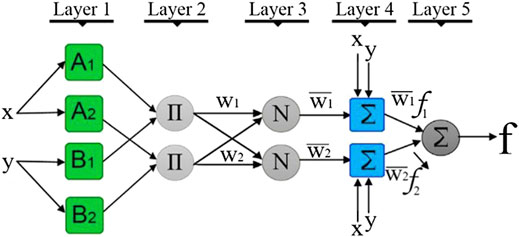
FIGURE 4. ANFIS model.

The functions of each layer in this ANFIS structure are introduced below (Abdulshahed et al., 2015):

Layer 1 is the input layer, which is intended for input fuzzification. In this layer, input variables are mapped into the fuzzy sets. Each node represents an adaptive node with node function.

${\mathrm{O}}_{\mathrm{1,}\mathit{i}}\mathrm{ = }{\mathrm{\mu }}_{\mathrm{A}\mathit{i}}\mathrm{ }\left(\mathit{x}\right)\mathrm{for}\mathit{i}\mathrm{ = 1, 2}(14)$

$\mathrm{or }{\mathrm{O}}_{\mathrm{1,}\mathit{i}}\mathit{ = }{\mathrm{\mu }}_{\mathrm{B}\mathit{i}}\mathit{ }\left(\mathit{y}\right)\mathrm{for }i=\mathrm{1,2}(15)$

x and y are the inputs for node i; O_1,i is the membership degree for fuzzy set A (membership functions A1, A2) or fuzzy set B (membership functions B1, B2). The typical bell-shaped membership function in this layer can be expressed as

${\mathit{\mu }}_A\left(x\right)=\frac{1}{1\mathrm{+}{\left|\frac{x-c_i}{a_i}\right|}^{2b_i}}(16)$

In Eq. 16, a, b, and c are the parameters for membership function u(x). These parameters determine the shape of the membership function and are referred to as premise parameters.

Layer 2 is the rule layer, which calculates the product of all the incoming signals to the nodes. Each node in this layer is a fixed node, and the output of this layer is the product of all the incoming signals or obtained from min (AND) in the fuzzy sets. Each node represents the firing strength of the rule. It can be calculated as

${\mathrm{O}}_{2,i}=\mathrm{wi}={\mathrm{\mu }}_{\mathrm{A}i}\left(x\right){\mathrm{\mu }}_{\mathrm{B}\mathit{i}}\mathrm{ }\left(\mathrm{y}\right)\mathrm{for }i=\mathrm{1,2}(17)$

$\mathrm{or }{\mathrm{O}}_{2,\mathrm{i}}={\mathrm{w}}_i=\min \left({\mathrm{\mu }}_{\mathrm{A}i}\left(x\right),{\mathrm{\mu }}_{\mathrm{B}\mathit{i}}\left(\mathrm{y}\right)\right)\mathrm{for }i=\mathrm{1,2}(18)$

Layer three is the normalization layer, which normalizes the firing strength of each node. Each node in this layer is also a fixed node, and the output is referred to as the normalized firing strength of that node. The output of the ith node is obtained by calculating the ratio of the ith rule'|’s firing strength to the sum of all rules' firing strengths. It can be calculated as

$O_{3,i}=\overline{w}=\frac{w_i}{w_1+w_2}\mathrm{for }\mathit{i}\mathrm{ = 1, 2}(19)$

Layer 4 is the inference layer, which is intended for defuzzification. Each node in this layer is an adaptive node. It takes the outputs from layer 3 and then multiplies them by the consequent parameters. It can be calculated as

$O_{4,i}={\overline{w}}_i{f}_i={\overline{w}}_i\left(p_{i}x+q_{i}y+r_i\right)(20)$

In Eq. 20, $\overline{w_i}$ is the normalized firing strength from layer 3 and {p_i, q_i, r_i} are the relevant consequent parameters for that node.

Layer 5 is the output layer, which calculates the overall output. There is only one fixed node in this layer. It calculates the overall output as the summation of all incoming signals and can be expressed as

$O_{5,i}={\displaystyle {\sum }_i{\overline{w}}_i{f}_i}=\frac{{\displaystyle {\sum }_i{w}_i{f}_i}}{{\displaystyle {\sum }_i{w}_i}}(21)$

In the ANFIS structure, the premise parameters are typically nonlinear, and consequent parameters are normally linear. This makes the parameter optimization process very complicated. Jang (Jang, 1993) proposes a hybrid learning algorithm to solve this problem. It involves a forward and backward process. In the forward pass, the premise parameters are first fixed, and the algorithm uses the least-squares method to identify the consequent parameters in Layer 4. After comparing the model output and desired output and obtaining the errors, the errors are propagated backward to the first layer, and the premise parameters are updated by the gradient descent method in the backward pass. This forward/backward process is repeated many times until the errors fall within the tolerance level. Since its introduction, ANFIS has been adopted to develop prediction models in many different research disciplines and is able to produce good prediction results (Vural et al., 2009; Boyacioglu and Avci, 2010; Abdulshahed et al., 2015).

Based on the related research, this research attempts to adopt three AI techniques (ANNs, SVMs, and ANFIS) to further investigate the relationship between in situ RH measurements and actual concrete compressive strength.

Data Collection

The researchers collaborated with a government-certified material testing laboratory and the Chinese Professional Civil Engineer Association for data collection. The RH tests were conducted on nonstructural beams in the basement of a large residential complex as shown in Figure 5. For consistency, all test hammer measurements were taken by the same personnel. The specifications in ASTM 805 and CNS 10732 for RH tests were carefully followed. After the RH tests, core samples were taken in order to obtain the actual compressive strength. To limit the structural damage due to coring, test locations were carefully chosen by the professional engineers. The design drawings were carefully reviewed to avoid rebar in the test areas. Before the test was conducted, test locations were examined again to avoid heavily textured or soft surfaces or surfaces with loose mortar. The digital RH was held firmly so that the plunger is perpendicular to the test surface. Ten readings were taken for each test area, and all the distances between impact points are greater than 25 mm. After each impact, the impression made on the surface was examined to see if the impact crushed or broke through a near-surface air void. If so, the reading was disregarded, and another reading was taken.

FIGURE 5

FIGURE 5. In situ rebound hammer test.

To obtain the actual compressive strength, core samples were also taken at the same location and then brought back to the laboratory for destructive compression tests. Design drawings were carefully reviewed, and professional engineers were consulted when determining the test locations (mostly within the middle third section of the beam). To avoid damage to the rebar, rebar detectors were employed to confirm the locations of rebar before drilling took place. In addition, the void was filled with low-shrinkage concrete right after the drilling. All of the core drillings were conducted by the same professional team from a local material testing laboratory. All the core samples were taken and prepared per the CNS 1238 A3051 (method of test for obtaining and testing drilled core samples of concrete) specifications. After cores were drilled, the surface water was wiped off, and the sample was stored in a nonabsorbent container. Before the compression tests, the ends of the core specimens were sawed so that they were flat and perpendicular to the longitudinal axis. The size of the test specimens is 7.5 Φ × 10 cm.

The basement is mainly intended for parking, and the building construction was approaching the completion stage when the tests were conducted. A total of 100 small beams were chosen for the RH tests, and these beams are have the same dimensions (50 cm in width and 70 cm in depth). For each beam, a total of 10 RH measurements were taken at one location. The Silver Schmidt N-Type electronic RH was used to conduct the tests. Core samples were taken at the same locations after the RH tests as shown in Figure 6. RH tests, core sample collection, and compression tests were conducted during a period of 4 weeks. These drilled core samples were taken back to the laboratory and carefully cured after the drill. To obtain the compressive strength, destructive compression tests were conducted using the HT-8391 200-ton concrete compression test machine. The data collected were used to develop and test the ANN, SVM, and ANFIS prediction models.

FIGURE 6

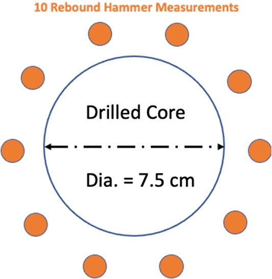
FIGURE 6. Rebound hammer and core sample location.

It should be noted that, before conducting the experiments, the research team were requested to sign a confidential agreement by the facility owner. As a result, only limited information regarding the research results can be revealed to the public. The descriptive statistics of RH tests and core sample compressive strength tests are shown in Table 1.

TABLE 1

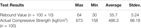
TABLE 1. Rebound hammer and core sample test results summary.

Model Development and Validation

A total of 100 RH test sample data were collected for this research analysis. The data are used to develop and validate the regression and artificial intelligence (ANNs, SVMs, and ANFIS) prediction models. Among the 100 samples, 80 of them are randomly chosen as the training data set, and the remaining 20 samples are assigned as the testing data set. For consistency, all the prediction models use the same 80 randomly selected samples to develop the models, and the same 20 samples are used to validate the models.

Some researchers have incorporated additional factors (such as water:cement ratio, aggregate size, and age) as input variables in their prediction models. Nevertheless, it is difficult (sometimes not feasible) to obtain these properties for existing structures. Therefore, this research only used RH measurements as the model inputs. For each test location, a total of 10 rebound measurements were taken as shown in Figure 6. These measurements were first recorded in the test hammer, and then the averages and standard deviations were calculated. All models proposed by this research have two input variables (average and standard deviation of the RH measurements) and one output variable (actual concrete compressive strength). As for the measure of model prediction accuracy, this research uses MAPE to compare prediction accuracies between the proposed models. MAPEs are widely used measures in examining the prediction accuracies for AI models (Nurcahyo and Nhita, 2014; Priya and Iqbal, 2015; Ramasamy et al., 2015). The MAPE is calculated using the following equation:

$MAPE=\frac{1}{n}{\displaystyle \sum _{i=1}^n\left|\frac{A_i-P_i}{A_i}\right|}(22)$

where A_i is actual compressive strength, P_i is model output, and n is the total number of data.

In addition to MAPE, root mean square error (RMSE) is also calculated as an alternative prediction measurement for models. Compared to MAPE, RMSE emphasizes large errors as shown in the following equation:

$RMSE=\sqrt{\frac{1}{n}{\displaystyle \sum }_{i=1}^n{\left(A_i-P_i\right)}^2}(23)$

Also, the variance accounted for (VAF) between the actual (desired) value and model prediction (output) is also calculated using the following equation (Kumar et al., 2013):

$VAF=\left(1-\frac{var\left(A-P\right)}{Var\left(A\right)}\right)\times 100\%(24)$

If the output values all equal the desired values, the MAPE and RMSE equal 0; the VAF equals 100%.

Regression Models

First, scatterplots of the collected data are plotted and examined for possible relationships between the average RH measurements and actual compressive strength. Next, simple linear and nonlinear regressions are conducted to see if simple regression models can yield good prediction results. The randomly chosen 80 training data are used to develop the linear and nonlinear regression models as shown in Figures 7, 8.

FIGURE 7

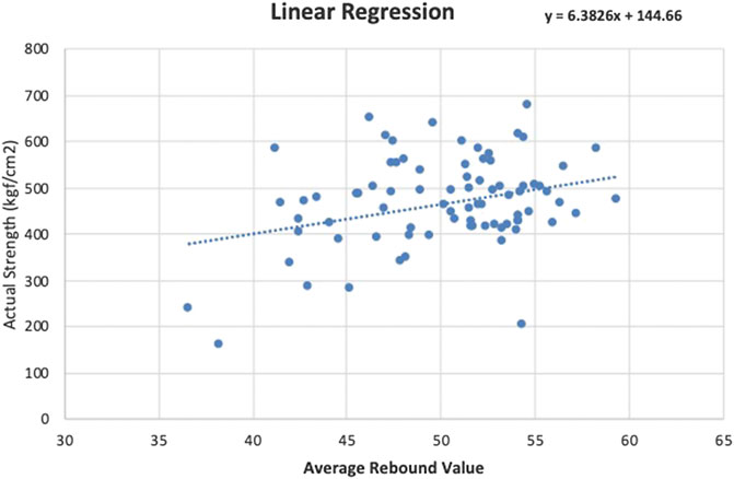
FIGURE 7. Linear regression scatterplot.

FIGURE 8

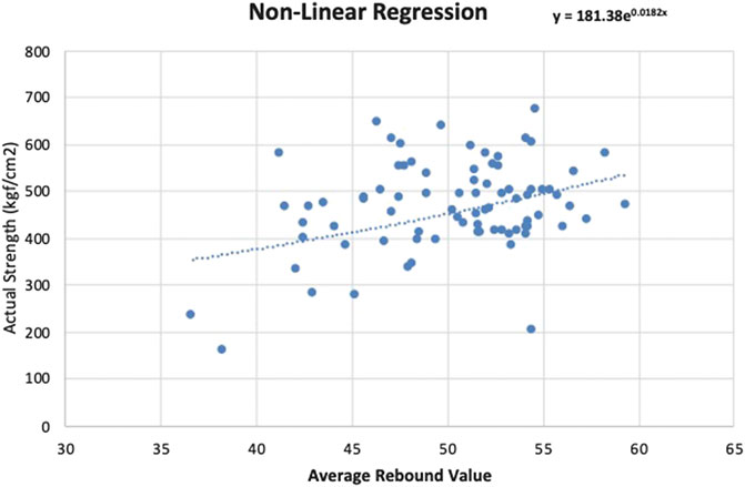
FIGURE 8. Nonlinear regression scatterplot.

The linear regression function obtained is

$y=6.3826x+144.6(25)$

For the linear regression model, the MAPE obtained from the training data is 17.88% and the RMSE is 90.81 kgf/cm².

The nonlinear regression function obtained is:

$y=181.38{\mathrm{e}}^{0.0182x}(26)$

For the nonlinear regression model, the MAPE obtained from the training data is 16.62% and the RMSE is 92.4 kgf/cm².

After obtaining the regression equations, the remaining 20 testing data are used to validate the regression models. The average rebound values from the testing data set are input into the equations to obtain concrete compressive strength predictions. The prediction results are then compared with the actual compressive strength obtained from the core sample destructive compression tests. The MAPE, VAF, and RMSE calculated for the linear regression model are 15.67%, ‒21.58%, and 103.07 kgf/cm², respectively. For the nonlinear regression models, the MAPE, VAF, and RMSE obtained are 16.75%, ‒19.13%, and 110.79 kgf/cm², respectively.

The prediction results show that both the linear and nonlinear regression models have MAPEs over 15%. Similar results are observed from other research indicating that traditional linear and nonlinear regression methods might not yield good prediction results (Wei, 2012; Mishra et al., 2019). In order to improve the prediction accuracy, this research proposes alternative prediction models based on AI methods (ANNs, SVMs, and ANFIS).

Artificial Neural Networks Models

This research uses NeuroSolutions 7.0 to develop the BP network (BPN) model for concrete compressive strength estimations. During the ANN model development process, parameters such as number of hidden layers, number of neurons in each layer, type of transfer functions, and learning rules are explored to obtain better prediction models. For this research, ANN models with both one and two hidden layers are developed. Different numbers of neurons in each layer, transfer functions, and learning rules are also investigated. In other words, trial and error is implemented to obtain better model parameter setup. Please refer to Table 2 for ANN model parameter setup details.

TABLE 2

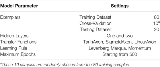
TABLE 2. ANNs model setup.

There are 80 samples in the training data set (including 10 cross-validation samples) and 20 samples in the testing data set. In order to find the best ANN prediction model, the ANN parameters are explored through the trial and error process. After several trials, it was found that better results (lower training errors) are obtained when using the “TanhAxon” transfer function and “Levenberg-Marquardt” (LM) learning rule. The TanhAxon transfer function applies a bias and tanh function to each neuron in the layer. This squashes the range of each neuron in the layer to between −1 and 1. The LM algorithm is a standard technique for nonlinear least-squares problems and can be thought of as a combination of steepest descent and the Gauss-Newton method.

The best training results obtained from the one-hidden-layer network is from a 2 to 5-1 (two inputs, five process elements in the hidden layer, and one output) ANN model. The MAPE and RMSE obtained are 16.82% and 101.21, respectively, from the training data set. This model is validated with the 20 samples using the testing data set. The MAPE, VAF, and RMSE obtained from the one-hidden-layer ANN model are 14.77%, −33.88%, and 92.67, respectively, when validating with the testing data.

ANN models with two hidden layers are also developed using the same training data set. Various parameter settings are explored in order to obtain lower training errors. The best training results obtained from the two-hidden-layer network is from a 2-5 to 5-1 (two inputs, five process elements in the first and second hidden layers, and one output) ANN model. The corresponding MAPE and RMSE obtained from the training data are 11.9% and 85.36, respectively, which are lower than the one-hidden-layer model. The training and validation errors for this ANN model are shown in Figure 9.

FIGURE 9

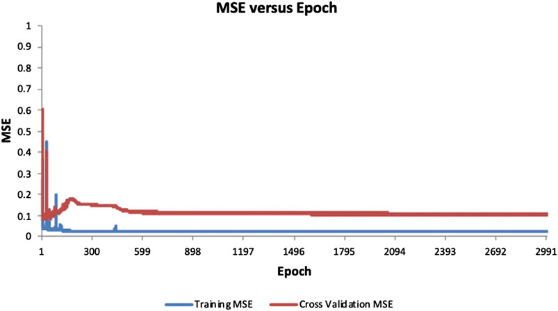
FIGURE 9. ANN model (2-5-5–1) training and validation error.

Next, the two-hidden-layer model is validated with the 20 samples from the testing data set. The MAPE, VAF, and RMSE obtained from the testing data are 12.37%, −30.68%, and 88.45, respectively, which are also lower than the one-hidden-layer model. The desired values (actual compressive strength) and model outputs are presented in a scatterplot as shown in Figure 10. If the model output equals the desired value, it should fall on the red line. In Figure 11, the line chart of the desired and model output compressive strengths is also plotted. To get a better understanding of the individual errors between the desired values and model outputs, a residual histogram of the testing samples is presented in Figure 12.

FIGURE 10

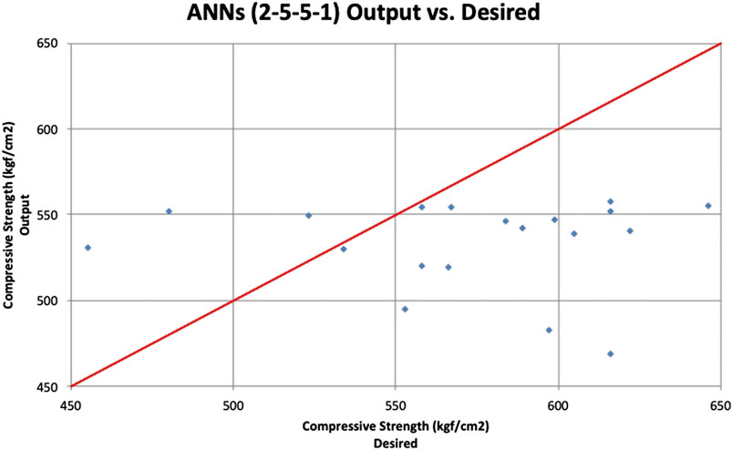
FIGURE 10. ANN model (2-5-5–1) scatterplot.

FIGURE 11

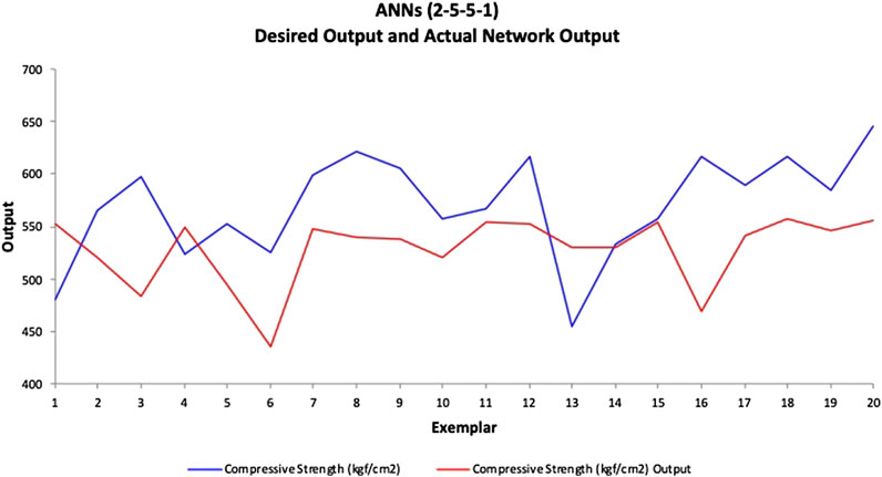
FIGURE 11. ANN model (2-5-5–1) line chart.

FIGURE 12

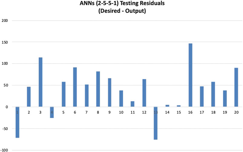
FIGURE 12. ANN model (2-5-5–1) residual histogram.

From the above, it can be observed that, most of the time, the predicted values (model outputs) are smaller than the desired values. It indicates that this ANN model tends to underestimate. In addition, there are 10 samples with residuals over 50 kgf/cm², which might contribute to the low prediction accuracy. The training and testing results of ANN models with one and two hidden layers are summarized in Table 3.

TABLE 3

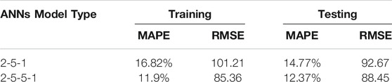
TABLE 3. ANNs model results.

Support Vector Regression Models

This research uses the least squares SVM (LSSVM) in the Matlab R2018a to develop the support vector regression model. The same 80 training data used in ANN model development are used to develop the LSSVM regression model.

For the SVM regression models, there are typically four types of kernel functions: linear, polynomial, sigmoid, and radial basis function (RBF) kernels. Among them, RBF is favorable for its capability of dealing with nonlinearity and high-dimensional computation and effectiveness in reducing complexity for inputs by adjusting C and γ (Hsu et al., 2003), where C is the cost of the soft-margin SVM loss function and gamma is the free parameter of the RBF. For this research, support vector regression parameters are obtained from the trial and error process. Different C and γ values are investigated to obtain the best SVM model with the training data set as shown in Table 4.

TABLE 4

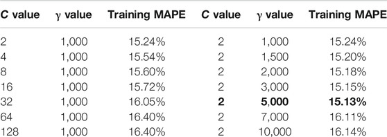
TABLE 4. SVM parameter settings and training error.

From Table 4, the best training MAPE obtained for the SVM model is 15.13%, and the corresponding C and γ values are 2 and 5,000, respectively.

Next, this model is validated with the 20 samples from the testing data set. The desired values (actual compressive strength) and support vector regression model outputs are presented in a scatterplot as shown in Figure 13. The red line indicates 100% accuracy prediction. The MAPE, VAF, and RMSE obtained for this support regression model are 16.08%, 6.05%, and 99.05, respectively. The line chart of the desired and model output compressive strengths is provided in Figure 14. The residual histogram of the testing samples is presented in Figure 15. The results show that the support vector regression model is not as accurate compared to the ANN model.

FIGURE 13

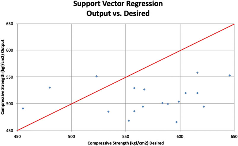
FIGURE 13. Support vector regression model scatterplot

FIGURE 14

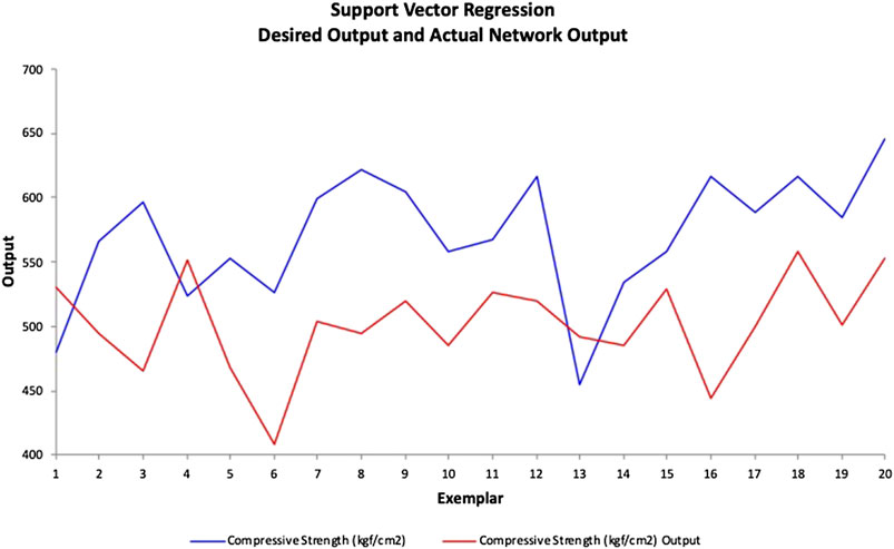
FIGURE 14. Support vector regression model line chart.

FIGURE 15

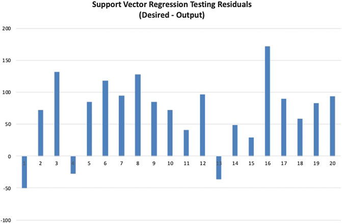
FIGURE 15. Support vector regression model residual histogram.

Adaptive Network-Based Fuzzy Inference Models

The ANFIS model is developed in the Matlab 2018a environment. The same 80 training samples used in ANN and SVM model development are also used to develop the ANFIS model. When developing the ANFIS models, the researchers can choose different numbers and types of membership functions. The researchers developed three different sets of models (models with three, five, and eight membership functions). For each membership function setting in Matlab 2018, there are eight different types to choose from: triangular (trimf), trapezoidal (trapmf), generalized bell-shaped (gbell), Gaussian (gauss1), Gaussian combination (gauss2), pi-shaped (pimf), difference between two sigmoidal (dsigmf), and product of two sigmoidal membership functions (psigmf). Each of them is tried in the ANFIS model development to find the best prediction results.

In the model setup, the tolerance level is set as 0, and the training is set to repeat 1,000, 2,000, and 3,000 times. The training error diagram for the model with three sigmoid membership functions (dsigmf) is shown in Figure 16.

FIGURE 16

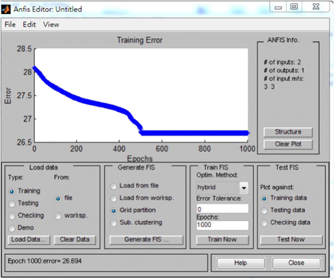
FIGURE 16. ANFIS model training error.

ANFIS models with three, five, and eight membership functions are developed using different types of membership functions. The models that yield the best training results are summarized in Table 5. For models with three membership functions ([3, 3]), the best MAPE, 10.45%, is obtained with the sigmoid membership functions (dsigmf). For models with five membership functions ([5, 5]), the best MAPE, 10.10%, is obtained with the trapezoidal membership functions (trapmf). For models with eight membership functions ([8, 8]), the best MAPE, 9.11%, is obtained with the trapmf membership function.

TABLE 5

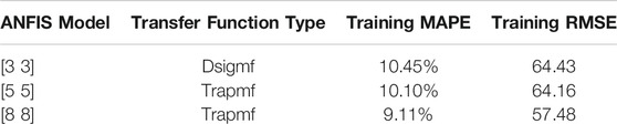
TABLE 5. ANFIS model training results.

After the best training model ([8, 8]), trapmf membership function) is identified, the remaining 20 testing samples (unseen data to the model) are used to obtain the concrete compressive strength predictions. The desired values (actual compressive strength) and support vector regression model outputs are presented in a scatterplot as shown in Figure 17. The line chart of the desired and ANFIS model output is provided in Figure 18. The residual histogram of the testing samples is presented in Figure 19. The MAPE, VAF, and RMSE obtained are 10.01%, −58.58%, and 62.46, respectively.

FIGURE 17

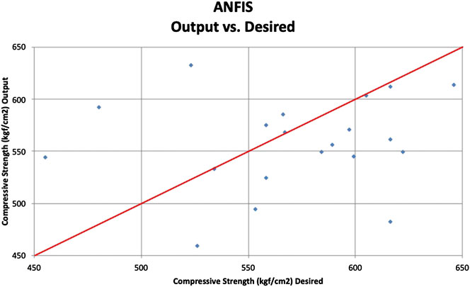
FIGURE 17. ANFIS model scatterplot

FIGURE 18

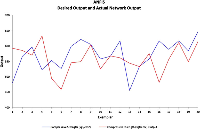
FIGURE 18. ANFIS model line chart.

FIGURE 19

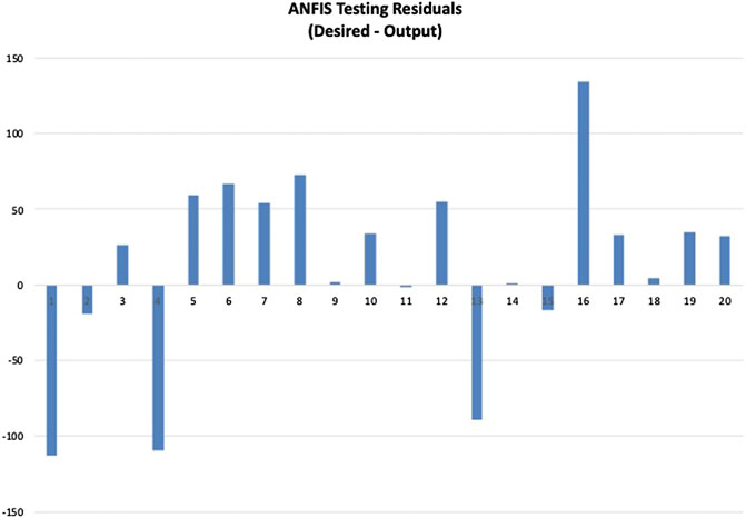
FIGURE 19. ANFIS model residual histogram.

The prediction results show that MAPEs in both training and testing data sets obtained from the three AI-based models are better than the 20% MAPE observed from previous research. Among them, the ANFIS model yields the best prediction accuracy with both the lowest training MAPE (9.11%) and testing MAPE (10.01%).

In order to examine the reliability of the prediction results, K-fold cross-validation is used to test the ANFIS model. In K-fold cross-validation, part of the available data is used to develop the model, and a different part of the data is used to test it. The K-fold cross-validation is also known as leave-one-out cross-validation (Hastie et al., 2009). For this research, the data are split into five equal-sized parts. Each of the five parts has 20 samples, and there are 100 samples in total. Four parts are first chosen to develop the prediction model, and the fifth part is used to calculate the prediction error. Then, another four parts are chosen to develop the model, and the remaining part is used to test the model. This process is repeated five times until all of the five parts are used to test the prediction model. The MAPE average and standard deviation of the five-fold cross-validation are 9.90% and 2.28%, respectively. The RMSE average and standard deviation of the five-fold cross-validation are 58.67 and 8.93, respectively. This result shows that, with different combinations of training and testing data, the ANFIS models are able to yield consistent prediction accuracies.

In summary, this research collected a total of 100 in situ RH and core sampling test data to develop concrete compressive estimation models. Among them, 80 samples were randomly selected to train the models, and the remaining 20 samples were used for model validation. First, linear and nonlinear regression models were developed and tested. The compressive strength prediction accuracies (measured by MAPE) obtained from the linear and nonlinear regression models are 15.66 and 16.75%, respectively, which do not show significant improvement from previous research. Subsequently, AI-based models (ANNs, SVMs, and ANFIS) were developed and validated using the same training and testing data sets. For each model, various model parameters were explored in order to achieve lower training error and higher prediction accuracy. Among these models, the ANFIS model yielded the best training and testing results with the lowest training and testing MAPEs of 9.11 and 10.01%, respectively. The model development and validation results from this research effort are summarized in Table 6. From Table 6, it can be observed that both ANN and ANFIS models are able to generate better prediction accuracies when compared to traditional linear and nonlinear regression models. Similar to Wei’s research results (Wei, 2012), the ANFIS model can produce the lowest prediction errors when using the RH measurement to measure concrete compressive strength.

TABLE 6

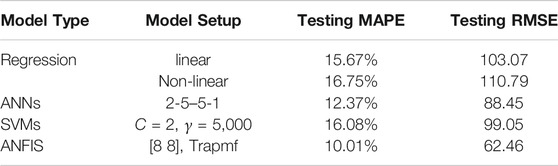
TABLE 6. Summary of model validation result.

Conclusions and Recommendations

To further investigate the relationship between in situ RH test measurements and actual concrete compressive strength, this research adopts AI techniques to develop concrete compressive strength prediction models. A total of 100 test data are collected from a large residential complex building. The data collected are used to develop and validate traditional regression models as well as AI-based models (ANN, SVM, and ANFIS models). For traditional regression models, the MAPEs calculated for the linear and nonlinear models are 15.66 and 16.75%, respectively. For the ANN model, the best prediction results are obtained from a two-hidden-layer network (2-5–5-1), and the MAPE obtained is 12.37%. For the support vector regression model, the best MAPE obtained is 16.08%. The corresponding parameters for the best support vector regression model are C = 2 and γ = 5,000. For this research, the ANFIS model yields the best prediction accuracy with an MAPE of 10.01% when the model is validated using the testing data. This result is obtained from the ANFIS model with eight membership functions for the two input variables ([8, 8]), and the membership function type is trapmf. K-fold cross-validation is also conducted, and the results show that the ANFIS model have consistent prediction errors when validated with different data. The research results show that AI techniques can be used to develop concrete compressive strength prediction models using in situ RH test measurements. The prediction accuracies are better when comparing to previous research results.

It should be noted that the RH test measurements are highly related to the near surface of the test object. Therefore, it is recommended that the RH tests can be combined with other nondestructive test methods (such as UPV tests) to improve concrete compressive strength estimations. Research results have shown that the SonReb (UPV + RH test) method (Rilem Report TC43-CND, 1993) might improve concrete strength estimations in NDT tests (Nobile, 2015; Rashid and Waqas, 2017; Pereira and Romão, 2018). For this research, the results are obtained from the 100-sample data collected. In order to improve reliability, it is suggested that more sample data could be collected for model development and validation.

Data Availability Statement

The datasets presented in this article are not readily available because confidential agreements are signed before the authors are allowed to conduct the experiments. Requests to access the datasets should be directed to yrwang@nkust.edu.tw.

Ethics Statement

Written informed consent was obtained from the individual(s) for the publication of any potentially identifiable images or data included in this article.

Author Contributions

Y-RW conceived the presented idea, supervised the experiments and analysis. Y-LL and D-LC conducted the experiment, developed the models and analyzed the data. Y-RW took the lead in writing the manuscript with help from Y-LL and D-LC.

Conflict of Interest

The authors declare that the research was conducted in the absence of any commercial or financial relationships that could be construed as a potential conflict of interest.

Acknowledgments

This material is based upon work supported by the Ministry of Science and Technology, TAIWAN under grant no. MOST 103‐2221‐E‐151‐053.

References

Abdulshahed, A. M., Longstaff, A. P., and Fletcher, S. (2015). The application of ANFIS prediction models for thermal error compensation on CNC machine tools. Appl. Soft Comput. 27, 158–168. doi:10.1016/j.asoc.2014.11.012.

CrossRef Full Text | Google Scholar

Abraham, A. (2005). Adaptation of fuzzy inference system using neural learning. Stud. Fuzziness Soft Comput. 181, 53–83. doi:10.1007/11339366_3.

CrossRef Full Text | Google Scholar

Anguita, D., Ghio, A., Greco, N., Oneto, L., and Ridella, S. (2010). “Model selection for support vector machines: advantages and disadvantages of the machine learning theory,”in The 2010 international joint conference on neural networks (IJCNN), Barcelona, Spain, July 18–23, 2010 (IEEE), 1–8.

Google Scholar

Asteris, P. G., and Mokos, V. G. (2019). Concrete compressive strength using artificial neural networks. Neural Comput. Applc. 32, 11807–11826. doi:10.1007/s00521-019-04663-2

CrossRef Full Text | Google Scholar

ASTM C597–16 (2020). Standard test for pulse velocity through concrete. Available at: http://web.archive.org/web/20190904130233/https://www.astm.org/Standards/C597.htm.

Google Scholar

ASTM C805/C805M (2020). Standard test method for rebound number of hardened concrete. Available at: http://web.archive.org/web/20190502123317/https://www.astm.org/Standards/C805.htm.

Google Scholar

Atoyebi, O. D., Ayanrinde, O. P., and Oluwafemi, J. (2019). Reliability comparison of schmidt rebound hammer as a non-destructive test with compressive strength tests for different concrete mix. J. Phys. Conf. 1378 (3), 032096. doi:10.1088/1742-6596/1378/3/032096.

CrossRef Full Text | Google Scholar

Balabin, R. M., and Lomakina, E. I. (2011). Support vector machine regression (SVR/LS-SVM)-an alternative to neural networks (ANN) for analytical chemistry? Comparison of nonlinear methods on near infrared (NIR) spectroscopy data. Analyst 136 (8), 1703–1712. doi:10.1039/c0an00387e.

PubMed Abstract | CrossRef Full Text | Google Scholar

Bishop, C. M. (2006). Pattern recognition and machine learning. Berlin, Germany: Springer.

Google Scholar

Boyacioglu, M. A., and Avci, D. (2010). An adaptive network-based fuzzy inference system (ANFIS) for the prediction of stock market return: the case of the Istanbul stock exchange, Expert Syst. Appl. 37 (12), 7908–7912. doi:10.1016/j.eswa.2010.04.045.

CrossRef Full Text | Google Scholar

Brencich, A., Cassini, G., Pera, D., and Riotto, G. (2013). Calibration and reliability of the rebound (Schmidt) hammer test. Civil Eng. Arch. 1 (3), 66–78. doi:10.13189/cea.2013.010303

Google Scholar

Breysse, D., and Martínez-Fernández, J. L. (2014). Assessing concrete strength with rebound hammer: review of key issues and ideas for more reliable conclusions. Mater. Struct. 47 (9), 1589–1604. doi:10.1617/s11527-013-0139-9.

CrossRef Full Text | Google Scholar

British Standards Institution (BSI) (1986). Testing concrete - Part 202: Recommendations for surface hardness testing by rebound hammer. BS 1881-202

Google Scholar

Drucker, H., Burges, C. C., Kaufman, L., Smola, A. J., and Vapnik, V. (1997). “Support vector regression machines,” in Advances in neural information processing systems. M., Mozer, M., Jordan, and T., Petsche (Cambridge, MA: MIT Press), 155–161.

Google Scholar

El Mir, A., and Nehme, S. G. (2017). Repeatability of the rebound surface hardness of concrete with alteration of concrete parameters. Construct. Build. Mater. 131, 317–326. doi:10.1016/j.conbuildmat.2016.11.085.

CrossRef Full Text | Google Scholar

European Normalization Committee (En) (2012). Testing concrete in structures - Part 2: non-destructive testing - determination of rebound number. EN 12504-2: 2012

Google Scholar

Gurney, K. (2014). An introduction to neural networks. Boca Raton, FL: CRC press.

Google Scholar

Hajjeh, H. R. (2012). Correlation between destructive and non-destructive strengths of concrete cubes using regression analysis. Contemp. Eng. Sci. 5 (10), 493–509.

Google Scholar

Hamidian, M., Shariati, A., Khanouki, M. A., Sinaei, H., Toghroli, A., and Nouri, K. (2012). Application of Schmidt rebound hammer and ultrasonic pulse velocity techniques for structural health monitoring. Sci. Res. Essays 7 (21), 1997–2001. doi:10.5897/SRE11.1387

CrossRef Full Text | Google Scholar

Hastie, T., Tibshirani, R., and Friedman, J. (2009). The elements of statistical learning: data mining, inference, and prediction. Berlin, Germany: Springer Science & Business Media.

Google Scholar

Hsu, C. W., Chang, C. C., and Lin, C. J. (2003). A practical guide to support vector classification. Tech. Rep. Department of Computer Science, National Taiwan University.

Google Scholar

Huang, W. L., Chang, C. Y., Chen, W. C., and We, C. N. (2011). Using ANNs to improve prediction accuracy for rebound hammers. Taiwan Highway Engineering 37 (2), 2–18.

Google Scholar

Huang, W., Nakamori, Y., and Wang, S.-Y. (2005). Forecasting stock market movement direction with support vector machine. Comput. Oper. Res., ; 32(10), p 2513–2522. doi:10.1016/j.cor.2004.03.016.

CrossRef Full Text | Google Scholar

Information on The Constructor (2012a). Rebound hammer test on concrete - principle, procedure, advantages & disadvantages. Availabe at: http://web.archive.org/web/20200221015718/https://theconstructor.org/concrete/rebound-hammer-test-concrete-ndt/2837/.

Google Scholar

Information on Gilson Company Inc. (2012b). Silver schmidt PC concrete test hammer. Availabe at: http://web.archive.org/web/20200221015938/https://www.globalgilson.com/silver-schmidt-pc-concrete-test-hammer-type-n

Google Scholar

Iphar, M. (2012). ANN and ANFIS performance prediction models for hydraulic impact hammers. Tunn. Undergr. Space Technol. 27 (1), 23–29. doi:10.1016/j.tust.2011.06.004.

CrossRef Full Text | Google Scholar

Jang, J.-S. R. (1993). ANFIS: adaptive-network-based fuzzy inference system. IEEE Trans. Syst. Man. Cybern. 23 (3), 665–685. doi:10.1109/21.256541.

CrossRef Full Text | Google Scholar

Kim, K. J. (2003). Financial time series forecasting using support vector machines. Neurocomputing 55 (1-2), 307–319. doi:10.1016/s0925-2312(03)00372-2.

CrossRef Full Text | Google Scholar

Kocáb, D., Misák, P., and Cikrle, P. (2019). Characteristic curve and its use in determining the compressive strength of concrete by the rebound hammer test. Materials 12 (17), 2705. doi:10.3390/ma12172705.

CrossRef Full Text | Google Scholar

Kumar, B. R., Vardhan, H., Govindaraj, M., and Vijay, G. S. (2013). Regression analysis and ANN models to predict rock properties from sound levels produced during drilling. Int. J. Rock Mech. Min. Sci. 58, 61–72. doi:10.1016/j.ijrmms.2012.10.002

CrossRef Full Text | Google Scholar

Kumar, C. V., Vardhan, H., and Murthy, C. S. (2019). Multiple regression model for prediction of rock properties using acoustic frequency during core drilling operations. Geomechanics and Geoengineering 15, 1–16. doi:10.1080/17486025.2019.1641631

CrossRef Full Text | Google Scholar

Mishra, M., Bhatia, A. S., and Maity, D. (2019). A comparative study of regression, neural network and neuro-fuzzy inference system for determining the compressive strength of brick–mortar masonry by fusing nondestructive testing data. Eng. Comput. doi:10.1007/s00366-019-00810-4.

CrossRef Full Text | Google Scholar

Nobile, L. (2015). Prediction of concrete compressive strength by combined non-destructive methods. Meccanica 50 (2), 411–417. doi:10.1007/s11012-014-9881-5.

CrossRef Full Text | Google Scholar

Nurcahyo, S., and Nhita, F. (2014). “Rainfall prediction in kemayoran jakarta using hybrid genetic algorithm (ga) and partially connected feedforward neural network (pcfnn),” 2nd International Conference on Information and Communication Technology (ICoICT). Bandung, Indonesia, May 28–30, 2014, 166–171.

Google Scholar

Pereira, N., and Romão, X. (2018). Assessing concrete strength variability in existing structures based on the results of NDTs. Construct. Build. Mater. 173, 786–800. doi:10.1016/j.conbuildmat.2018.04.055.

CrossRef Full Text | Google Scholar

Priya, S. S., and Iqbal, M. H. (2015). Solar radiation prediction using artificial neural network. Int. J. Comput. Appl. 116 (16), p 28–31. doi:10.5120/20422-2722

CrossRef Full Text | Google Scholar

Qasrawi, H. Y. (2000). Concrete strength by combined nondestructive methods simply and reliably predicted. Cement Concr. Res. 30 (5), 739–746. doi:10.1016/s0008-8846(00)00226-x.

CrossRef Full Text | Google Scholar

Ramasamy, P., Chandel, S. S., and Yadav, A. K. (2015). Wind speed prediction in the mountainous region of India using an artificial neural network model. Renew. Energy 80, 338–347. doi:10.1016/j.renene.2015.02.034.

CrossRef Full Text | Google Scholar

Rashid, K., and Waqas, R. (2017). Compressive strength evaluation by non-destructive techniques: an automated approach in construction industry. J.Build. Eng. 12, 147–154. doi:10.1016/j.jobe.2017.05.010.

CrossRef Full Text | Google Scholar

Rezaeianzadeh, M., Tabari, H., Arabi Yazdi, A., Isik, S., and Kalin, L. (2014). Flood flow forecasting using ANN, ANFIS and regression models. Neural Comput. Appl. 25 (1), 25–37. doi:10.1007/s00521-013-1443-6.

CrossRef Full Text | Google Scholar

RILEM Recommendation. (1993). Draft recommendation for in situ concrete strength determination by combined non-destructive methods. Mater. Struct, 26, 43–49.

Google Scholar

Rojas-Henao, L., Fernández-Gómez, J., and López-Agüí, J. C (2012). Rebound hammer, pulse velocity, and core tests in self-consolidating concrete. ACI Mater. J. 109 (2), 235–243. doi:10.14359/51683710

Google Scholar

Shariati, M., Ramli-Sulong, N. H., Kh, M. M. A., Shafigh, P., and Sinaei, H. (2011). Assessing the strength of reinforced concrete structures through ultrasonic pulse velocity and schmidt rebound hammer tests. Sci. Res. Essays 6 (1), 213–220. doi:10.5897/SRE10.879

CrossRef Full Text | Google Scholar

Shirsath, P. B., and Singh, A. K. (2010). A comparative study of daily pan evaporation estimation using ANN, regression and climate based models. Water Resour. Manag. 24 (8), 1571–1581. doi:10.1007/s11269-009-9514-2.

CrossRef Full Text | Google Scholar

Smola, A. J., and Schölkopf, B. (2004). A tutorial on support vector regression. Stat. Comput. 14 (3), 199–222. doi:10.1023/b:stco.0000035301.49549.88.

CrossRef Full Text | Google Scholar

Szilágyi, K., Borosnyói, A., and Zsigovics, I. (2011). Rebound surface hardness of concrete: introduction of an empirical constitutive model. Construct. Build. Mater. 25 (5), 2480–2487. doi:10.1016/j.conbuildmat.2010.11.070.

CrossRef Full Text | Google Scholar

The National Standards of the Republic of China (1986). Chinese National Standards (CNS). Methods of test for rebound number of Hardened Concrete. CNS 10732‐1984, Taiwan: CNS

Google Scholar

Topçu, İ. B., and Sarıdemir, M. (2008). Prediction of compressive strength of concrete containing fly ash using artificial neural networks and fuzzy logic. Comput. Mater. Sci. 41 (3), 305–311. doi:10.1016/j.commatsci.2007.04.009.

CrossRef Full Text | Google Scholar

Vapnik, V. (2013). The nature of statistical learning theory. Berlin, Germany: Springer science & business media.

Google Scholar

Vural, Y., Ingham, D. B., and Pourkashanian, M. (2009). Performance prediction of a proton exchange membrane fuel cell using the ANFIS model. Int. J. Hydrogen Energy 34 (22), 9181–9187. doi:10.1016/j.ijhydene.2009.08.096.

CrossRef Full Text | Google Scholar

Wei, S. H. (2012). Application of the adaptive neuro-fuzzy inference system model in predicting the concrete compressive strength from the silverschmidt hammer. Master thesis. Kaohsiung (Taiwan): National Kaohsiung University of Applied Sciences

Google Scholar

Xu, T., and Li, J. (2018). Assessing the spatial variability of the concrete by the rebound hammer test and compression test of drilled cores. Construct. Build. Mater. 188, 820–832. doi:10.1016/j.conbuildmat.2018.08.138.

CrossRef Full Text | Google Scholar

Yılmaz, I., and Yuksek, A. G. (2008). An example of artificial neural network (ANN) application for indirect estimation of rock parameters. Rock Mech. Rock Eng. 41 (5), 781–795. doi:10.1007/s00603-007-0138-7

CrossRef Full Text | Google Scholar

Yilmaz, I., and Kaynar, O. (2011). Multiple regression, ANN (RBF, MLP) and ANFIS models for prediction of swell potential of clayey soils. Expert Systems with Applications 38 (5), 5958–5966. doi:10.1016/j.eswa.2010.11.027.

CrossRef Full Text | Google Scholar

Zupan, J., and Gasteiger, J. (1991). Neural networks: a new method for solving chemical problems or just a passing phase?. Anal. Chim. Acta 248 (1), 1–30. doi:10.1016/s0003-2670(00)80865-x.

CrossRef Full Text | Google Scholar