A Deep Belief network and Least Squares Support Vector Machine Method for Quantitative Evaluation of Defects in Titanium Sheet Using Eddy Current Scan Image

Introduction

Titanium (Ti) is an ideal structural material with excellent all-round properties, such as low density, high specific strength, and excellent corrosion resistance (Cui et al., 2011). For decades, Ti was mainly used in the aerospace and defense industries (Malwina, 2016). Later, as its production increased, it was also gradually applied to other fields, such as the chemical and medical industries, and ocean and civil engineering (Gurrappa, 2003; Veiga et al., 2012; Bayrak and Yilgor Huri, 2018). In civil engineering, Ti sheets can be safely connected with ceramics, glass, and concrete because all of these materials have similar thermal expansion coefficients (Winowiecka and Adamus, 2016). As a result, the Ti sheet structures constructed are not only light and beautiful but can also be made resistant to chemical pollution, acid rain, and marine corrosion (Adamus, 2014); this construction method has been successfully applied to marine buildings and earthquake-proof constructions around the world (Adamus, 2014; Malwina, 2016). Despite the excellent all-round properties of Ti sheets, defects are inevitably produced during long-term use. In order to ascertain the remaining life of the Ti sheets, it is important to characterize the dimensions of Ti sheet defects. Therefore, a method for effectively detecting and evaluating Ti sheet defects is indispensable.

Eddy current testing (ECT) is a nondestructive testing method based on electromagnetic induction (Sophian et al., 2001), which has been widely used for detecting and evaluating defects in conductive parts of engineered structures. Compared with other nondestructive testing methods, ECT has many advantages, such as no contact, low cost, and no pollution (Fan et al., 2016). In ECT, the characterization of a material defect is considered to be an inverse problem, in which the defect dimensions are retrieved from the detected signals (Tian et al., 2005). Traditionally, the dimensions of a defect have been estimated by visual judgment of ECT detection signals by an inspector. This method usually requires highly trained personnel, and the results are usually influenced by the subjectivity of the inspector (Fan et al., 2016). Thus, some researchers have turned to machine learning methods to deal with the ECT inverse problem. In these methods, defect feature extraction mainly relies on a manual design or simple signal processing methods, such as principal component analysis (PCA) and independent component analysis (ICA) (Tian et al., 2005; Sophian et al., 2003; He et al., 2013; Daura and Tian, 2019), while the quantitative evaluation of defects mainly employs conventional machine learning methods, such as artificial neural network (ANN) and Bayesian network (Wrzuszczak and Wrzuszczak, 2005; Khan and Ramuhalli, 2008). In recent years, improved visualization methods for ECT have been developed that can accurately and intuitively reflect the shape, degree, and position of defects, while keeping the original advantages of ECT. Bodruzzaman et al. reported a neural network–based method for estimating the dimension of cracks in metal plates using eddy current (EC) scan images (Bodruzzaman and Zein-Sabatto, 2008). Diraison et al. presented an EC imager designed for defect evaluation of aeronautical lap joints, with PCA used to extract the EC image features for defect characterization (Diraison et al., 2009). He et al. investigated pulsed EC (PEC) imaging, with defect evaluation performed based on the morphological features of EC scan images (He et al., 2011). Ye et al. used a giant magnetoresistance (GMR) array to image crack defects in the inner wall of a steam generator tube and evaluated the crack depth using the amplitude of the defect area in the EC image (Ye et al., 2016). Nafiah et al. used PEC testing to obtain an EC scan image of an inclined crack, and then, three image-based features were designed to characterize the inclination and depth of the crack (Nafiah et al., 2019). With improvements in ECT scanning speed, the EC image contains more information, and there are discrepancies in image quality under different working conditions. Therefore, extracting effective features using an artificial design or simple signal processing becomes difficult, which affects the efficacy of quantitative evaluation.

To solve the above problem, deep learning seems to be a good solution. Because deep learning methods have powerful nonlinear characterization and self-learning capabilities, they are very useful for extracting essential features from high-dimensional nonlinear data (Cheng et al., 2019). In 2006, Hinton et al. discussed the deep learning theory for the first time and proposed a deep belief network (DBN) built from multiple stacked restricted Boltzmann machines (RBMs) to solve the difficulty of deep network training and optimization (Hinton et al., 2006; Hinton and Salakhutdinov, 2006). To date, deep learning has achieved good performance in many fields, such as image recognition, voice detection, and fault diagnosis (Zhang and Wu, 2013; O'Connor et al., 2013; Chen and Li, 2017; Wu et al., 2020). These valid theoretical foundations and successful applications provide new ideas for the ECT field. Currently, combining deep learning with the ECT technology is a trend in the future development of modern civil engineering material testing. Therefore, in this article, we propose a method that combines the EC scan imaging technology with a quantitative evaluation method for Ti sheet defect evaluation based on DBNs and least squares support vector machine (LSSVM). First, unsupervised self-learning was conducted on multiple RBMs layer by layer, and the trained RBMs were stacked to construct a multilayer DBN, before conducting supervised fine-tuning. Then, defect features were extracted from the EC scan images of Ti sheets using the trained DBN. Finally, based on the extracted feature vectors, a multi-objective regression model of defect dimensions was established using the LSSVM algorithm. This combination of effective features and an efficient regression model was used to perform the quantitative evaluation of Ti sheet defects. Detection and evaluation experiments were conducted on Ti sheets with different degrees of defects to confirm the validity of the proposed method. The proposed method does not require manually design features, avoiding inspector subjectivity. Furthermore, the deep learning method provides essential and concise features, leading to higher accuracy and reliability for the proposed method than for conventional methods.

The remainder of the work is arranged as follows: the DBN used for feature extraction and LSSVM used for multi-objective regression of defect dimensions are briefly introduced in Section 2; then, the experimental setup and materials are described in Section 3; in Section 4, the experimental results are described and discussed; and finally, conclusions and further potential work are outlined in Section 5.

Method

Restricted Boltzmann Machine

An RBM (Hinton, 2012) is a basic unit constituting the DBN and can be regarded as a neural network containing a visible layer and a hidden layer, with the number of neurons in the hidden layer usually being smaller than that in the visible layer. The main purpose of an RBM is to compress a given data set and to minimize the reconstruction error so as to obtain the effective features of the original data set. The structure of an RBM is shown in Figure 1.

FIGURE 1

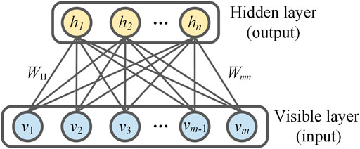
FIGURE 1. Structure of an restricted Boltzmann machine.

According to Figure 1, combined with EC scan imaging, the visible layer represents a column vector of a rearranged EC image, while the hidden layer represents the features after dimension reduction. There is a bidirectional symmetric connection between the two layers of the RBM, with no connections within each of the layers. An RBM is an energy-based model (Zhang and Wu, 2013), with the layer-by-layer learning process following the energy function expressions:

$E\left(\mathbf{v},\mathbf{h}|\theta \right)=-{\displaystyle \sum _{i=1}^m{a}_i{v}_i-}{\displaystyle \sum _{j=1}^n{b}_j{h}_j}-{\displaystyle \sum _{i=1}^m{\displaystyle \sum _{j=1}^n{v}_i{W}_{ij}{h}_j}},(1)$

where θ = {W = (W_ij)_{m × n}, a = (a_ij)_{1 × m}, and b = (b_i)_{1 × n}} are the model parameters; v_i and a_i are the state and bias of the ith neuron in the visible layer, respectively; h_i and b_i are the state and bias of the jth neuron in the hidden layer, respectively; W_ij is the connection weight between the ith visible neuron and the jth hidden neuron; and m and n are the number of neurons in the visible and hidden layers, respectively.

Based on the above energy function, the joint probability distribution of the RBM over the visible and hidden neurons is defined as follows:

$P\left(\mathbf{v},\mathbf{h}|\theta \right)=\frac{e^{-E\left(v,h|\theta \right)}}{{\displaystyle \sum _v{\displaystyle \sum _h{e}^{-E\left(v,h|\theta \right)}}}}.(2)$

Due to the structure of the RBM model (full connectivity between layers and no connectivity within layers), when the state of visible neurons is given, the activation state of each hidden neuron is conditionally independent, and vice versa (Chen and Li, 2017). Therefore, the conditional probabilities over hidden and visible neurons are given by

$\{\begin{array}{c}P\left(h_j=1|\mathbf{v},\theta \right)=sig\left(b_j+{\displaystyle {\sum }_i{v}_i{W}_{ij}}\right)\\ P\left(v_i=1|\mathbf{h},\theta \right)=sig\left(a_i+{\displaystyle {\sum }_j{W}_{ij}}{h}_j\right)\end{array},(3)$

where $sig\left(x\right)$ is a sigmoid function, which is selected as the activation function in this study.

RBM training involves adjusting the parameter θ. The training objective is to maximize the likelihood function $L\left(\theta |\widehat{\mathbf{v}}\right)=P\left(\mathbf{v}=\widehat{\mathbf{v}}|\theta \right)$ using the gradient descent algorithm (O'Connor et al., 2013). Suppose the input data are ${\mathbf{v}}^t={\left(v_1^t,v_2^t,\cdots ,v_m^t\right)}^T,t=\mathrm{1,2},\cdots ,N$, the calculation of gradients is performed according to the following equations:

$\{\begin{array}{c}\frac{\partial \ln L\left(\theta |{\mathbf{v}}^t\right)}{\partial W_{ij}}=P\left(h_j=1|{\mathbf{v}}^t\right)v_i^t-{\displaystyle {\sum }_{v}P\left(\mathbf{v}\right)P\left(h_j=1|\mathbf{v}\right)v_i},\\ \frac{\partial \ln L\left(\theta |{\mathbf{v}}^t\right)}{\partial a_i}=v_i^t-{\displaystyle {\sum }_{v}P\left(\mathbf{v}\right)v_i},\text{ and}\\ \frac{\partial \ln L\left(\theta |{\mathbf{v}}^t\right)}{\partial b_j}=P\left(h_j=1|{\mathbf{v}}^t\right)-{\displaystyle {\sum }_{v}P\left(\mathbf{v}\right)P\left(h_j=1|\mathbf{v}\right)}.\end{array}(4)$

The calculation of P(v) in Eq 4 is very complicated. In this study, contrastive divergence (CD) (Hinton, 2002) is used to provide an approximate estimation. During training, the parameter θ is updated according to the following equations:

$\{\begin{array}{c}{W}_{ij}=W_{ij}+ϵ\frac{\partial \ln L\left(\theta |v^t\right)}{\partial W_{ij}}\\ a_i=a_i+\frac{\partial \ln L\left(\theta |v^t\right)}{\partial a_i}\\ b_j=b_j+ϵ\frac{\partial \ln L\left(\theta |v^t\right)}{\partial b_j}\end{array},(5)$

where ε > 0 is the learning rate.

Deep Belief Network

A DBN is a deep network composed of multiple RBMs and is a feedforward neural network algorithm with the advantages of multiple hidden layers and fast training (Hinton et al., 2006). Due to a large number of pixels and discrepancy in quality of EC scan images, it is difficult to obtain effective defect features via self-learning using only one RBM. Therefore, in this study, a DBN containing multiple hidden layers is constructed by stacking multiple RBMs, which realize self-learning of effective features layer by layer. Figure 2 shows a DBN comprising three stacked layers of RBMs. The training process for a DBN consists of two stages (Hinton et al., 2006): the unsupervised pretraining stage and the supervised fine-tuning stage:

(1) Pretraining uses the layer-by-layer greedy algorithm (Bengio et al., 2007) to train each RBM separately. When the training of the first layer of an RBM is completed, its output is taken as the input of the next layer of the RBM, and then, this process of transmission continues layer by layer. During the training of each layer of an RBM, the gradient is calculated according to Eq 4 and the parameters are updated according to Eq 5.

(2) After pretraining, multiple RBMs are stacked, and a logic layer is added as the top layer to construct a DBN containing multiple hidden layers. The stacking of RBMs described above can be understood as initializing a deep neural network with the connection weights of multiple RBMs as an initial weight of the deep neural network. Then, the back propagation (BP) algorithm and the batch gradient descent method are used to fine-tune the network. During the training process, the error is back-propagated to each layer of the RBM from high to low, with the parameters between each layer adjusted until the maximum number of iterations is reached, to achieve the optimal DBN model

FIGURE 2

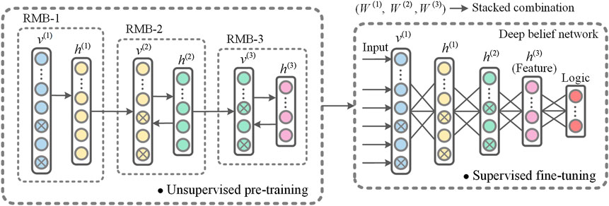
FIGURE 2. Deep belief network structure.

Least Squares Support Vector Machine

The LSSVM (Suykens and Vandewalle, 1999) is an improved version of the general SVM. It transforms the quadratic programming problem arising from the constraint conditions of the traditional SVM to the problem of solving linear equations, which greatly improves the solution speed (Haifeng and Dejin, 2005). In many cases, the relationship between defects and features is very complex and nonlinear, making it difficult to build an effective mathematical model. Therefore, the LSSVM algorithm is used in this study to establish a multiple-objective regression model using the extracted features, allowing for the quantitative evaluation of defects.

For the input sample set (x_i, y_i), i = 1, 2, … , l, x_i and y_i indicate the feature vector and defect parameters of the ith EC scan image, and l is the total number of samples. The nonlinear mapping Φ maps the features to a feature space, with the regression model expressed as

$y=f\left(x\right)={\omega }^T\mathrm{\Phi }\left(x\right)+b.(6)$

Determining unknown parameters ω and b is equivalent to solving the following optimal problem:

$\{\begin{array}{l}\min \frac{1}{2}\left({\Vert \omega \Vert }^2+\gamma {\displaystyle \sum _{i=1}^l{e}_i^2}\right)\\ s.t.{\omega }^T\mathrm{\Phi }\left(x_i\right)+b+e_i=y_i,i=\mathrm{1,2},\cdots ,l\end{array},(7)$

where γ is the regularization parameter controlling the penalty degree of error, ω is the weight vector, Φ is a kernel function, b is the bias, and e_i is the error variable. To solve this optimization problem, the Lagrange multiplier is introduced to construct a Lagrange function:

$L\left(\omega ,b,e,\alpha \right)=\frac{1}{2}\left({\Vert \omega \Vert }^2+\gamma {\displaystyle \sum _{i=1}^l{e}_i^2}\right)-{\displaystyle \sum _{i=1}^l{\alpha }_i}\left({\omega }^T\mathrm{\Phi }\left(x_i\right)+b+e_i-y_i\right).(8)$

According to the Karush–Kuhn–Tucker (KKT) condition for solving the nonlinear programming problem, the equation for solving ω and b is obtained as follows (Suykens and Vandewalle, 1999):

$\left[\begin{array}{llll}I\hfill & 0\hfill & 0\hfill & -Z\hfill \\ 0\hfill & 0\hfill & 0\hfill & L\hfill \\ 0\hfill & 0\hfill & \gamma I\hfill & -I\hfill \\ Z^T\hfill & L^T\hfill & I\hfill & 0\hfill \end{array}\right]\left[\begin{array}{l}\omega \hfill \\ b\hfill \\ e\hfill \\ \alpha \hfill \end{array}\right]=\left[\begin{array}{l}0\hfill \\ 0\hfill \\ 0\hfill \\ y\hfill \end{array}\right],(9)$

where I is an unit vector of l order, L = [1,1, … ,1], α = [α₁,α₂, … ,α_l]^T, and Z = [Φ(x₁), Φ(x₂), …, Φ(x_l)]. By eliminating ω and e, Eq 8 can be simplified as follows:

$\left[\begin{array}{ll}0\hfill & L\hfill \\ L^T\hfill & Z^{T}Z+\frac{1}{\gamma }I\hfill \end{array}\right]\left[\begin{array}{l}b\hfill \\ \alpha \hfill \end{array}\right]=\left[\begin{array}{l}0\hfill \\ y\hfill \end{array}\right],(10)$

where Z^TZ = k(x_i, x_j), with k being the kernel function of LSSVM.

Since the quantitative evaluation of defects in Ti sheets has obvious nonlinear characteristics, the radial basis kernel function was chosen as k:

$k\left(x_i,x_j\right)=\exp \left(-\frac{\Vert x-x_i\Vert }{2{\delta }^2}\right),(11)$

where δ² is the kernel parameter. Support vector coefficients α and bias b can be obtained by solving the above linear equations to determine the regression model as follows:

$y=f\left(x\right)={\displaystyle \sum _{i=1}^l{\alpha }_i}k\left(x,x_i\right)+b.(12)$

Quantitative Evaluation of Ti Sheet Defects Based on Deep Belief Network and Least Squares Support Vector Machine

Considering the high information content and discrepancy in quality of EC scan images, we propose a method for the quantitative evaluation of Ti sheet defects based on the DBN and LSSVM combined with EC scan imaging. This method stacks multiple RBMs to construct a DBN with multiple layers, with the deep network being trained via unsupervised self-learning and supervised fine-tuning. The trained DBN can fit nonlinear functions well, so it is used to extract the potential high-order features from EC scan images. Based on the extracted features, a multi-objective regression model of defect dimensions (length, diameter, and depth) is established using the LSSVM. The effective features and efficient regression model are then combined to achieve the quantitative evaluation of Ti sheet defects. In line with the description given above, the specific steps of the quantitative evaluation method are shown in Figure 3.

FIGURE 3

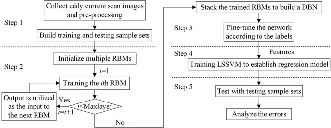
FIGURE 3. Flowchart of the proposed method.

As shown in Figure 3, the main steps carried out to implement this method are as follows:

(1) EC imaging testing is performed on different Ti sheet defects to obtain EC scan images. After preprocessing (such as de-noising), the training and testing samples are constructed.

(2) Multiple RBMs are initialized, and the training samples are input into the first-layer RBM for training. After the training of the first-layer RBM is complete, its output is used as the input for the next-layer RBM, and the training is continued. This process is repeated until the training of all of the RBMs is complete.

(3) Multiple trained RBMs are stacked, and a logic layer is added to construct a DBN containing multiple hidden layers, which is then fine-tuned using the labels of the training samples.

(4) The trained DBN is used to extract features from the training samples; based on these features, a regression model of defect dimensions is established using the LSSVM algorithm.

(5) The above methods are then tested by using the DBN to extract features of the testing samples, which are input into the LSSVM model to obtain quantitative evaluation results. Finally, error analysis is conducted on the results.

Experimental Setup and Materials

The entire detection system used in this study is shown in Figure 4, consisting of a programmable scanning stage, a stage controller, an EC probe, a host PC, and an electromagnetic (EM) instrument. The EM instrument was developed by the Sensing, Imaging, and Signal Processing Group at the School of Electrical and Electronic Engineering at the University of Manchester (Yin and Peyton, 2006; Yin et al., 2011). The EM instrument can operate at frequencies of 5–200 kHz and can perform digital demodulation at a rate of 100 k/s (Yin et al., 2019).

FIGURE 4

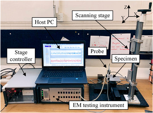
FIGURE 4. Experimental detection system.

The probe used in the above system is a transmitter–receiver (T-R)–type probe composed of two coils: one for excitation and the other for pickup. A schematic of the T-R probe is shown in Figure 5. Compared with absolute probes with a single coil, T-R probes have a higher gain, have a wider frequency range, and are unaffected by thermal drift (Cao et al., 2018). In addition, the spatial resolution of T-R probes along a scan line is almost twice as high as that of absolute probes with the same coil size. These characteristics make the T-R probes more suitable for imaging applications (Cheng et al., 2017). Although the T-R probes have good performance, their detection effect is also affected by coil parameters such as coil radius, coil gap, and lift-off of the probe. The parameters of T-R probes should be selected as needed.

FIGURE 5

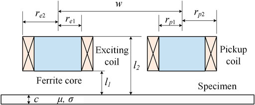
FIGURE 5. Structure of eddy current probe.

The larger the coil, the lower the working frequency required for maximum sensitivity; however, it also results in a reduction in spatial resolution (Xu et al., 2018). Considering the dimensions of the smallest defect in the specimen used in this study, the inner radius of the coils was chosen to be 0.75 mm. The outer radius of the coils is related to coil turns to ensure sufficient signal strength. After coil processing, the outer radius of transmitter and receiver coils was 1.25 and 1.50 mm, respectively. In addition, the sensitivity decreases and the lift-off resistance increases with the increase in coil gap (Ona et al., 2019). After testing, the receiving coil voltage was greatest at the smallest coil gap of 2.75 mm and almost zero when the coil gap was greater than 10.00 mm. Following consideration of the balance of sensitivity and lift-off resistance, a median value of 3.50 mm was taken as the coil gap. With a decided coil gap, the voltage variation in the receiver coil will be maximized at a certain lift-off. For the above coil gap, the voltage variation achieves its maximum at a lift-off of 0.50 mm. According to the above analysis, the parameters of the T-R probe used in this study are determined and listed in Table 1.

TABLE 1

TABLE 1. Probe parameters.

In order to simulate defects of different types and degrees, two representative types of defects were selected for processing in two Ti specimens. As shown in Figure 6, cracks and holes were machined in two 3.0-mm-thick Ti (TA2) sheets via electrical discharge machining, respectively. Each specimen contained nine defects of different dimensions. From Figure 6A, the width of all cracks was 1.0 mm, while the length of each row was 4.0, 8.0, and 12.0 mm, respectively, and the depth of each column was 0.5, 1.5, and 2.5 mm, respectively; from Figure 6B, the hole diameter of each row was 1.0, 2.0, and 3.0 mm, respectively, and the depth of each column was 0.5, 1.5, and 2.5 mm, respectively. The numbers and parameters of defects are listed in Table 2.

FIGURE 6

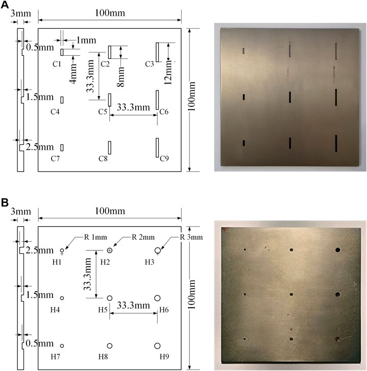
FIGURE 6. Machined specimen: (A) specimen #1; (B) specimen #2.

TABLE 2

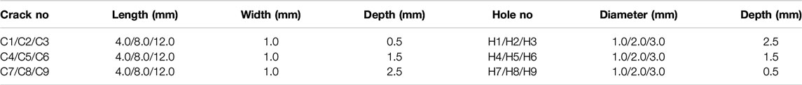
TABLE 2. Parameters of defects.

The T-R probe used in this study is a directional sensor, and the detection mainly relies on the coupling of coils and eddy current, which are predominant in the middle part of two coils. During the scanning process, to facilitate the description, the direction of the connection line between the two coil centers is defined as the probe direction, as shown in Figure 7A. When the transmitter coil of the T-R probe approaches a defect, the EC is cut off by the defect, as shown in Figure 7B. The severed EC is concentrated at the edge of the crack, and the EC density in the middle part of the two coils is stronger than that in the other areas. If the probe direction is along the scan direction, the concentrated EC in the middle of the two coils is propitious to strengthen the coupling between the transmitter and receiver coils. If the probe direction is perpendicular to the scan direction, as shown in Figure 7C, the T-R probe is under completely different operation conditions. The receiver coil is away from the area where the EC is concentrated. Thus, the mutual coupling between the transmitter and receiver coils was significantly reduced under the influence of eddy current, and the sensitivity of the receiver coil, which is in the perpendicular direction, decreases significantly.

FIGURE 7

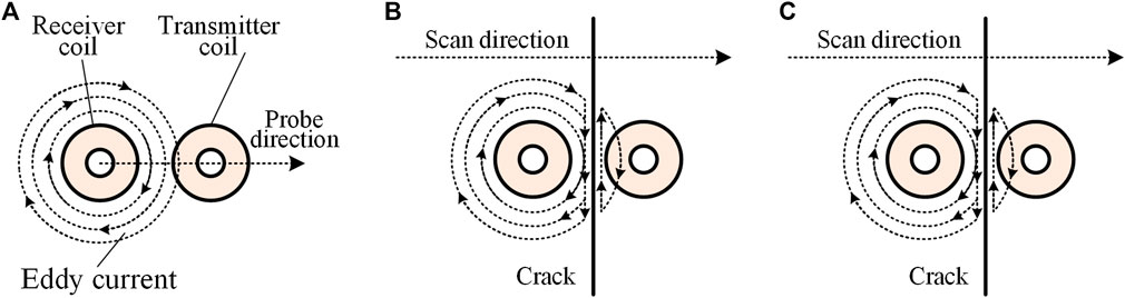
FIGURE 7. Influence of T-R probe direction: (A) probe direction definition; (B) probe direction is along the scan direction; (C) probe direction is perpendicular to the scan direction.

According to the above discussion, the scan mode used in the experiments is shown in Figure 8. Better performance of scan detection can be obtained if the scan direction is along the probe direction, which makes the voltage variation in the receiver coil to be greater when the T-R probe moves to a defect. In this way, defects in the EC scan image will also be better represented. From Figure 8, during the experimental measurement, the scan stage was driven by the stage controller to move the probe to scan the specimen: the steps in the X and Y directions were 0.40 and 1.25 mm, respectively, and the scanning points for each defect were arranged in a 40 × 20 grid (covering a 15.60-mm area × 23.75-mm area).

FIGURE 8

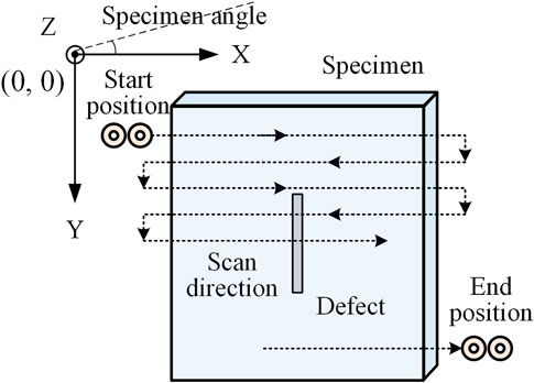
FIGURE 8. Scan mode.

During the scanning process, the EM instrument provided a sine voltage output to the excitation coil of the T-R probe, thereby generating an alternating magnetic field over the specimen. The induced EC generates a magnetic field opposite to the original magnetic field, and the pickup coil receives the resultant magnetic flux. The resultant magnetic flux varies in the presence of a defect, thus changing the induced voltage in the pickup coil. Then, the pickup coil voltage was sampled by the analog-to-digital converter (ADC) in the EM instrument. At the same time, two quadrature reference signals with the same frequency as excitation were generated in the processor of the EM instrument. The two reference signals were input into the digital phase-sensitive detection (PSD) module together with the sampling signal. The real and imaginary parts of the sampling signal were obtained by mixing and integrating the sampling signal and each reference signal. Finally, the real and the imaginary parts of the signals were transmitted to the host PC via an Ethernet interface.

In addition, the working frequency of ECT determines the skin depth and detection accuracy. Generally, the lower the working frequency, the greater the skin depth, but the smaller the detection precision. The selection of working frequency depends on the thickness and electromagnetic characteristics of the measured material. The expression of the standard skin depth δ is given as follows:

$\delta =1/\sqrt{\pi f{\mu }_0{\mu }_r\sigma },(13)$

where f is the working frequency; σ and μ_r are the conductivity and relative permeability of the measured material, respectively; and μ₀ is the permeability of free space.

In the experiment, the thickness of the Ti (TA2) specimen is 3.0 mm, the conductivity is 1.8 MS/m, and the relative permeability is 1. The standard skin depth was selected as 0.7 times the thickness of the specimen to prevent EC from appearing on the other side of the specimen and to ensure the depth and accuracy of the detection. According to Eq 13, the working frequency used for the EM instrument in the experiment carried out in this study was 30 kHz.

Experimental Results

A defect in a Ti sheet causes a change in the voltage of the pickup coil. However, for different materials, the sensitivity of the real and imaginary parts of the voltage differs. In order to determine the more sensitive signal components, we first carried out a line scanning along the vertical direction of three defects. Defects with the minimum length and different depths were selected as examples (C1, C4, and C7 defects in specimen #1) and referenced to Ti sheets without defects; the differences in the pickup coil voltages are shown in Figure 9.

FIGURE 9

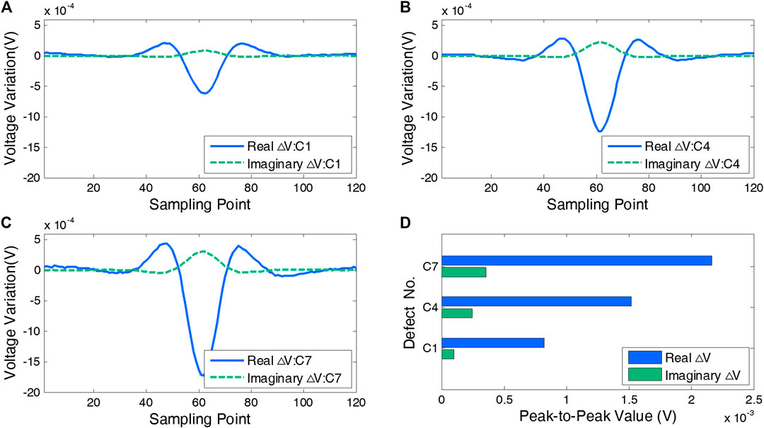
FIGURE 9. Signal strength comparison: (A) real and imaginary parts of voltage difference for C1 notch; (B) real and imaginary parts of voltage difference for C4 notch; (C) real and imaginary parts of voltage difference for C7 notch; (D) comparison of peak-to-peak values.

From Figures 9A–C, it can be seen that the real and imaginary parts of the coil voltage difference reach the peak value at the defect center and that the trend of the change is opposite to this. However, the peak-to-peak value of the real part is much larger than that of the imaginary part. As shown in Figure 9D, the peak-to-peak value of the real part is on average five times greater than that of the imaginary part. From this, it can be concluded that the real part of the peak-to-peak value is more sensitive at detecting defects in Ti sheets. According to the preliminary testing mentioned above, visualization of defects can be improved by using the difference in the real part because the stronger signals are not as easily drowned out by environmental noise.

The scan mode described in Figure 8 was adopted to scan the different defects in the two specimens. However, in actual detection, differences in manual operations will result in discrepancies in the quality of the scan images. Such situations were simulated by scanning each defect at different angles and from different start positions to provide experimental samples for subsequent evaluation, where the angle refers to the angle between the specimen and the scan direction, from 0 to 25° with an interval of 5°, and the X and Y axis coordinates of the start position change in the range of −2 to 2 mm with an interval of 2 mm. With six angles and nine start position combinations, each scan was repeated five times. In total, 270 samples were obtained for each defect: 200 samples of each defect were randomly selected as the training data, and the remaining 70 samples were used as the testing data. Finally, for each specimen, the total number of training samples was 1,800 and the number of testing samples was 630. After the above scan process was completed, taking the scanning image with the start position of (0,0) and scanning angle of 0° as an example, the imaging effect of the two specimens is shown in Figure 10.

FIGURE 10

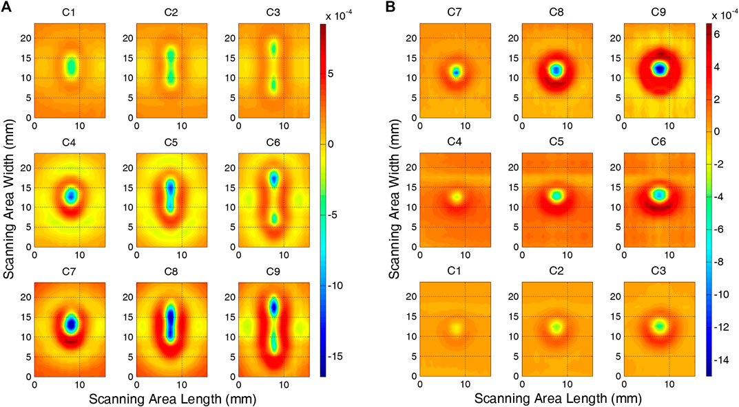
FIGURE 10. Imaging effect: (A) specimen #1 (crack defects); (B) specimen #2 (hole defects).

Figures 10A,B show the nine crack defects and nine hole defects in specimens #1 and #2, respectively. In Figures 10A,B, each panel represents the imaging effect of the defect of the corresponding number, allowing the shape and depth of defects to be intuitively assessed in EC scan images. For the defects with the same shape, the defect regions in EC scan images had relatively similar contours. For the defects with the same depth, the defect regions in EC scan images had similar pixel value distribution, and as the defect depth increases, the color value of the defect region in EC scan image gradually decreases.

Before the experiments of feature extraction and quantitative evaluation, how the parameters in the DBN and LSSVM affect the performance of the proposed method was first discussed and analyzed. The network structure is the most important factor for the DBN and is related to the number of hidden neurons and the number of layers. Since each RBM in the DBN is independently trained, taking the first RBM to construct a DBN as an example, an experiment was conducted to determine the appropriate number of hidden neurons. The input layer and the output layer were set to 800 and nine neurons, respectively, representing the input data dimension and the binary-coded defect type. The hidden neurons were set to 50–700 at a step of 50. The mean square error (MSE) between output code and actual code is used to evaluate feature characterization ability of the DBN. The mean results of two specimens are shown in Figure 11. It is noted that the feature characterization results seem to be satisfactory when the number of neurons in the hidden layer is less than 1/4th that in the previous layer.

FIGURE 11

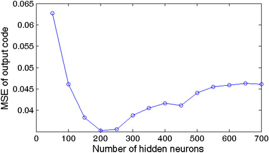
FIGURE 11. Mean square error (MSE) curves of different numbers of hidden neurons.

Based on the analysis above, the number of hidden layers in the DBN was set to 1–3, and their network structure was 800/200/9, 800/200/50/9, and 800/200/50/12/9, respectively. An experiment was conducted to analyze the influence of the number of hidden layers on the deep learning structure. The results for each experimental condition are shown in Figure 12. It is noted that the results seem to be best when the number of hidden layers is 2.

FIGURE 12

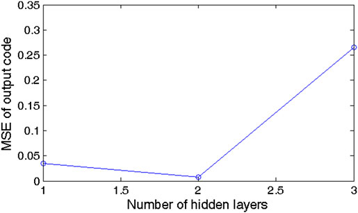
FIGURE 12. Mean square error curves of different numbers of hidden layers.

Learning rate plays an important role in the DBN to determine whether and when the objective function converges to the minimum; momentum factor determines the direction and efficiency of gradient descent. So, a suitable learning rate and momentum factor could not only improve the learning ability but also enhance the computing efficiency. Taking all of the above results together, further experiments of the learning rate and momentum factor were conducted. In the experiments, the learning rate was set to 0.05–1.00 in the pretraining and fine-tuning stages; when one stage was analyzed, the learning rate of the other stage remained unchanged, which was 1.00; the momentum factor was set to 0.05–1.00 in pretraining and fine-tuning stages. The results of the experiments above are shown in Figures 13 and 14, respectively.

FIGURE 13

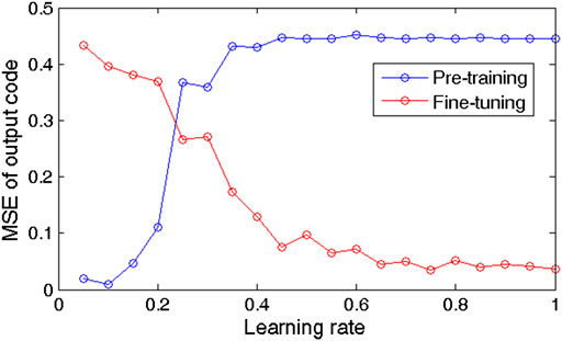
FIGURE 13. MSE curves of different numbers of learning rate.

FIGURE 14

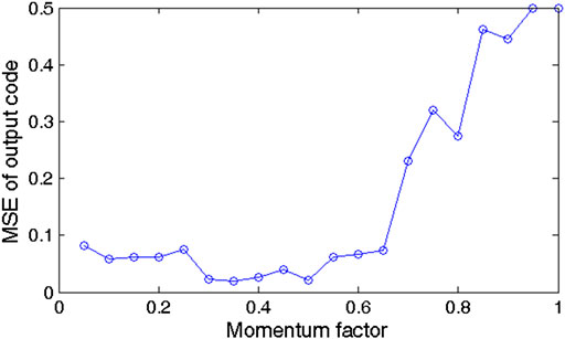
FIGURE 14. MSE curves of different numbers of momentum factor.

From Figure 13, in the pretraining stage, the MSE increases with the increase in the learning rate, and the MSE becomes stable gradually after the learning rate is greater than 0.35. In addition, the MSE achieves its minimum of 0.01 at a learning rate of 0.10. In the fine-tuning stage, the MSE decreases with the increase in the learning rate. As the learning rate varies from 0.70 to 1.00, the MSE clearly decreases, with a result of 0.037–0.049, and the MSE shows little variation when the learning rate continues to increase. From Figure 14, when the momentum factor was taken as an intermediate value, the MSE is the smallest, and the MSE achieves its minimum of 0.021 at a momentum factor of 0.50.

After the above analysis and preliminary experiment, the DBN used in this experiment was set to contain two hidden layers, and the outputs of the last hidden layer were the extracted features. Detailed parameters of the DBN are listed in Table 3.

TABLE 3

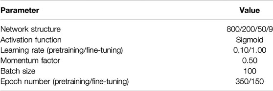
TABLE 3. Parameters of deep belief network model.

In LSSVM algorithm, the regularization parameter and kernel parameter directly affect the learning and generalization ability. Besides, there is no necessary relationship between the regularization parameter and kernel parameter. Thus, they can be analyzed and discussed independently. A DBN model with the parameters in Table 3 was trained by training samples. The trained DBN model was used to extract features from the training and testing samples. The features from the training samples were used to establish the LSSVM regression model, and the features from the testing samples were used to analyze how the parameters affect the LSSVM. The regularization parameter was set to 0.1–20.0, and the kernel parameter was set to 0.05–2.50. According to the above parameter settings, the relative errors of defect evaluation by using the LSSVM are shown in Figures 15 and 16.

FIGURE 15

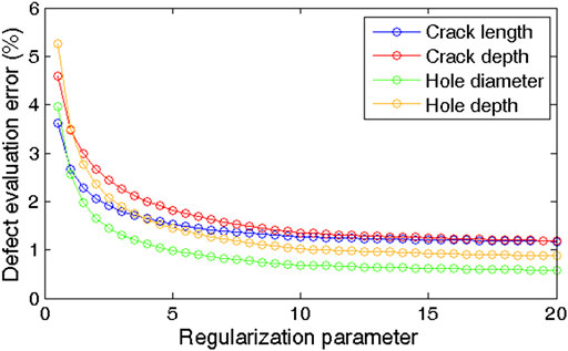
FIGURE 15. Defect evaluation results of different regularization parameters.

FIGURE 16

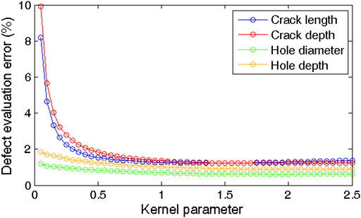
FIGURE 16. Defect evaluation results of different kernel parameters.

From Figure 15, the relative error of defect evaluation decreases with the increase in the regularization parameter. For both crack and hole defects, the relative error decreases obviously in the range of the regularization parameter from 0.5 to 12.0, and the relative error shows little variation when the regularization parameter continues to increase. From Figure 16, the variation in relative error with the kernel parameter is similar to the above description of the regularization parameter. The relative error shows little variation when the kernel parameter is greater than 1.00 and achieves its minimum at a kernel parameter of 1.50. So, we determine that the regularization parameter and kernel parameter of the LSSVM are 10.0 and 1.50, respectively.

After the above preliminary experiments, we analyzed the effects of parameters in the DBN and LSSVM on the performance of the proposed method and determined the optimal parameters. Next, the feature extraction and defect quantitative evaluation experiments were carried out. A trained DBN model was used to extract features from the EC scan images in the testing samples. In addition, in this experiment, PCA, ANN, and single-layer RBM were used for comparison, where the number of neurons in each layer of the ANN was set to 800/200/50/9 and the structure of the RBM was set to 800/50, with the other parameters being the same as those in the DBN. To visualize the distribution of features, the obtained features were mapped to 3D feature vectors, taking specimen #1 as an example, and the results are shown in Figure 17.

FIGURE 17

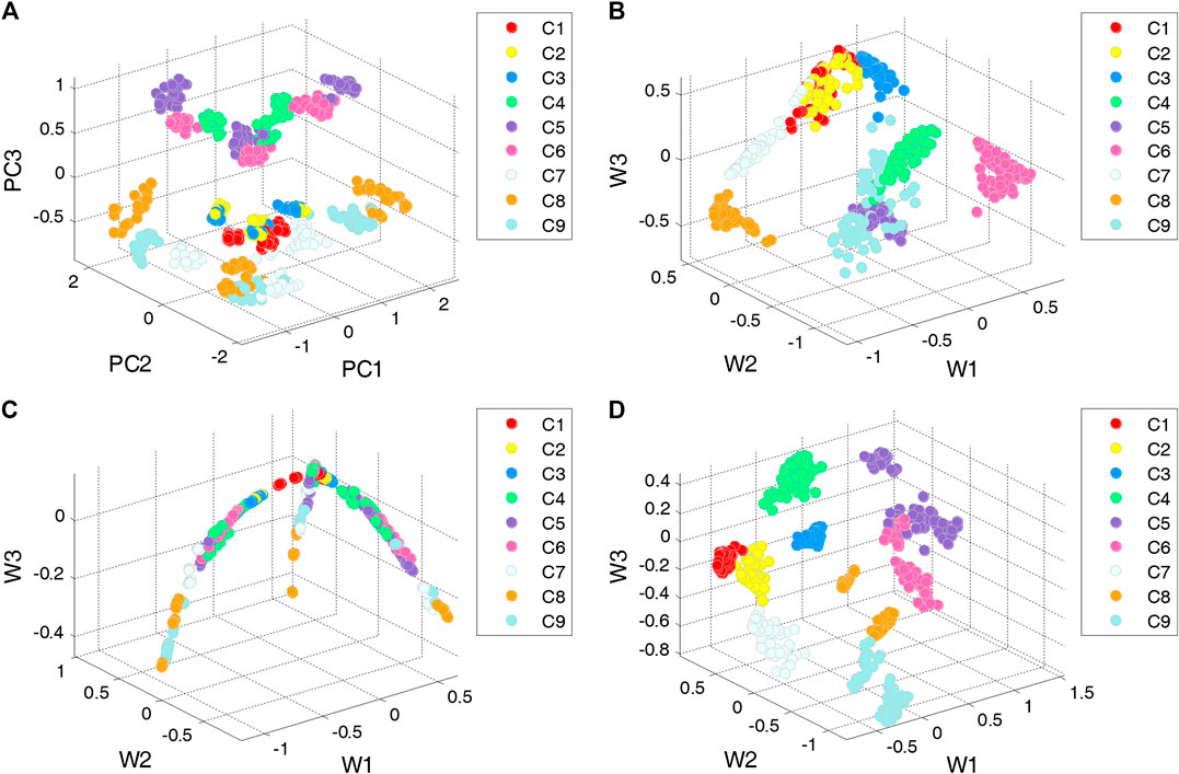
FIGURE 17. Comparison of feature extraction effects: (A) PCA; (B) ANN; (C) RBM; (D) DBN.

From Figure 17, it can be seen that the defect features extracted by PCA were relatively mixed, which shows that this method has difficulty in processing high-dimensional nonlinear data. The features of the same defect extracted by the ANN were obviously clustered, but for different defects, there were some overlaps of between-class features. The features extracted by the RBM formed a curve-like distribution, also with some overlaps of between-class features when there were too many defect types. The performance of the DBN model was better than that of the other models; this is mainly because the unsupervised self-learning of the DBN (based on its deep structure) is conducive to characterizing the essential and concise high-order features, while the supervised learning of the DBN improves the clustering of inner-class feature sets. Therefore, the features extracted by the DBN are more suitable for the quantitative evaluation of defects.

The extracted features from EC scan images of two specimens were input into the previously established LSSVM regression model to quantitatively evaluate the Ti sheet defects. This experiment involved performing a multi-objective regression task to evaluate the lengths and depths of the crack defects, and the diameters and depths of the hole defects. Table 4 shows the relative errors of the estimation results.

TABLE 4

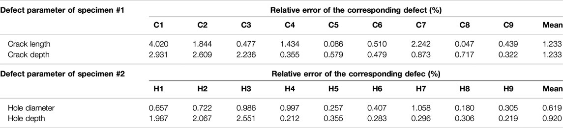
TABLE 4. Relative error of the defect evaluation of deep belief network–least squares support vector machine.

As shown in Table 4, the relative errors of estimation of crack length were between 0.047 and 4.020%, and those of crack depth were between 0.322 and 2.931%; the relative errors of estimation of hole diameter were between 0.180 and 0.997%, and those of the hole depth were between 0.212 and 2.551%. Overall, larger deviations were observed in the estimation of smaller degrees of defects (smaller in length/diameter and depth), and the mean relative errors of the above estimations were 1.233, 1.233, 0.619, and 0.920%, respectively; all errors are very small and within a reasonable range. Then, the above method was compared with other methods. In the comparison experiments, the four types of features (PCA, ANN, RBM, and DBN) described in Figure 17 were used, and two regression methods, multiple linear regression (MLR) and LSSVM, were used to reconstruct the defect dimensions. Table 5 shows the mean relative errors of the evaluation results for a total of eight groups of comparison experiments.

TABLE 5

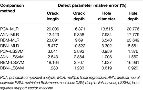
TABLE 5. Mean relative error of the defect evaluation of the comparison methods.

As shown in Table 5, in terms of the features used in these methods, the performance of the methods using PCA or ANN features is similar. Compared with the above features, the performance of RBM features is relatively weak, which indicates that the single-layer RBM is difficult to approximate high-order functions and extract effective features. In addition, the DBN feature has the best performance, and the errors of reconstructed defect dimensions are the smallest, no matter which regression algorithm was used. In terms of the regression algorithm used in these methods, the LSSVM is much better than MLR, and the average error is one order of magnitude smaller, which indicates that the LSSVM is more suitable for dealing with the nonlinear relationship between high-dimensional features and defect dimensions.

These results were further analyzed to evaluate the repeatability of the proposed method. The experiments were repeated under identical conditions, with the standard deviation used to evaluate the repeatability of the proposed method, and the results are shown in Table 6.

TABLE 6

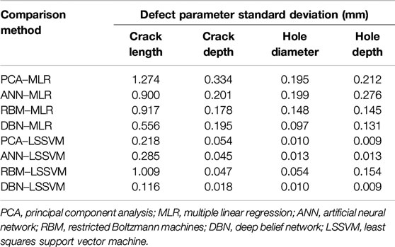
TABLE 6. Repeatability of the evaluation methods.

As shown in Table 5, the standard deviations of the experimental results for the DBN–LSSVM method ranged from 0.009 to 0.116 mm for the different defect parameters. These values are far below those of other comparison methods, demonstrating that the results of the proposed method do not readily fluctuate and show better repeatability. All in all, the above experiments prove the validity of the proposed method from the two aspects of accuracy and repeatability. The proposed method can be applied to perform effective detection and quantitative evaluation of Ti sheet defects, providing a novel way of combining deep learning with the EC scan imaging technology.

Conclusion

This study proposed a method for quantitatively evaluating Ti sheet defects based on the DBN and LSSVM combined with the EC scan imaging technology. The proposed method utilizes a trained DBN to extract effective features from the EC scan images of Ti sheet defects. Then, based on the extracted feature vectors, the LSSVM algorithm was used to establish a multi-objective regression model of the dimensions of the Ti sheet defects. The combination of effective features and an efficient regression model was used to perform the quantitative evaluation of Ti sheet defects. The main conclusions of this study are as follows:

(1) For defects in Ti materials, the strength of the real part of the detection signal is on average five times greater than that of the imaginary part. Therefore, the real part of the signal is not easily drowned out by environmental noise and can therefore achieve better imaging results. Furthermore, it is also better suited to the quantitative evaluation of defects based on features extracted from EC scan images.

(2) The proposed method does not require manually designed features, thus avoiding the problem of the subjectivity of the inspector. In addition, compared with feature extraction by conventional methods, the proposed method stacks multiple RBMs and combines unsupervised and supervised learning, giving it a stronger ability to characterize features.

(3) The proposed method utilizes the LSSVM algorithm to transform the complex ill-posed ECT inverse problem to a simple problem of solving linear equations. The final experimental results showed that the maximum relative error and standard deviation of the defect evaluation were less than 4.1% and 0.12 mm, respectively, and the proposed method yielded a higher accuracy and repeatability than the other conventional methods tested.

In addition, due to limitations in our capacity to process the specimen, the defects studied in this research were all regular, ideal defects. However, defects often have more complex shapes in actual situations. We hope that future work will be able to extend the proposed method to investigate more complex defects. Second, the method should not be limited to the detection of Ti sheets in civil engineering but can also be extended to other ECT applications, such as reinspection and quality monitoring in the manufacturing of various metal sheets. In industrial production, with the accumulation of EC image data, the training samples will be enriched and the generalization capability of the proposed method will be further improved. We hope that future work will also focus on how to extend the proposed method to more ECT applications.

Data Availability Statement

The raw data supporting the conclusions of this article will be made available by the authors, without undue reservation.

Author Contributions

JB proposed the idea and wrote the original manuscript. BY designed the experiments and the titanium sheet specimen. JB and BY analyzed the data. XW and JW guided the research and were tasked with the critical revisions of the manuscript.

Conflict of Interest

The authors declare that the research was conducted in the absence of any commercial or financial relationships that could be construed as a potential conflict of interest.

Funding

This work was supported in part by the National Natural Science Foundation of China under Grant 51465024 and in part by the Applied Basic Research Programs of Science and Technology Commission Foundation of Yunnan Province under Grant 2019FB081.

Acknowledgments

The authors would like to acknowledge Wuliang Yin (School of Electrical and Electronic Engineering, University of Manchester, United Kingdom) for his help and the experimental instrument provided.

References

Adamus, J. (2014). Applications of titanium sheets in modern building construction. Adv. Magn. Reson. 1020, 9–14. doi:10.4028/www.scientific.net/AMR.1020.9

CrossRef Full Text | Google Scholar

Bayrak, E., and Yilgor Huri, P. (2018). Engineering musculoskeletal tissue interfaces. Front. Mater. 5. doi:10.3389/fmats.2018.00024

CrossRef Full Text | Google Scholar

Bengio, Y., Lamblin, P., Popovici, D., and Larochelle, H. (2007). “Greedy layer-wise training of deep networks,” in Proceedings of the Advances in neural information processing systems.

Google Scholar

Bodruzzaman, M., and Zein-Sabatto, S. (2008). “Estimation of micro-crack lengths using eddy current c-scan images and neural-wavelet transform,” in Proceedings of the IEEE SoutheastCon. doi:10.1109/SECON.2008.4494355

CrossRef Full Text | Google Scholar

Cao, B.-H., Li, C., Fan, M.-B., Ye, B., and Tian, G.-Y. (2018). Analytical model of tilted driver-pickup coils for eddy current nondestructive evaluation. Chin. Phys. B 27, 030301. doi:10.1088/1674-1056/27/3/030301

CrossRef Full Text | Google Scholar

Chen, Z., and Li, W. (2017). Multisensor feature fusion for bearing fault diagnosis using sparse autoencoder and deep belief network. IEEE Trans. Instrum. Meas. 66, 1693–1702. doi:10.1109/TIM.2017.2669947

CrossRef Full Text | Google Scholar

Cheng, J., Qiu, J., Ji, H., Wang, E., Takagi, T., and Uchimoto, T. (2017). Application of low frequency ect method in noncontact detection and visualization of CFRP material. Compos. B. Eng. 110, 141–152. doi:10.1016/j.compositesb.2016.11.018

CrossRef Full Text | Google Scholar

Cheng, Y., Zhu, H., Wu, J., and Shao, X. (2019). Machine health monitoring using adaptive kernel spectral clustering and deep long short-term memory recurrent neural networks. IEEE Trans. Ind. Inf. 15, 987–997. doi:10.1109/TII.2018.2866549

CrossRef Full Text | Google Scholar

Cui, C., Hu, B., Zhao, L., and Liu, S. (2011). Titanium alloy production technology, market prospects and industry development. Mater. Des. 32, 1684–1691. doi:10.1016/j.matdes.2010.09.011

CrossRef Full Text | Google Scholar

Daura, L. U., and Tian, G. Y. (2019). Wireless power transfer based non-destructive evaluation of cracks in aluminum material. IEEE Sensor. J. 19, 10529–10536. doi:10.1109/JSEN.2019.2930738

CrossRef Full Text | Google Scholar

Diraison, Y. L., Joubert, P.-Y., and Placko, D. (2009). Characterization of subsurface defects in aeronautical riveted lap-joints using multi-frequency eddy current imaging. NDT E Int. 42, 133–140. doi:10.1016/j.ndteint.2008.10.005

CrossRef Full Text | Google Scholar

Fan, M., Wang, Q., Cao, B., Ye, B., Sunny, A., and Tian, G. (2016). Frequency optimization for enhancement of surface defect classification using the eddy current technique. Sensors 16, 649. doi:10.3390/s16050649

CrossRef Full Text | Google Scholar

Gurrappa, I. (2003). Characterization of titanium alloy ti-6al-4v for chemical, marine and industrial applications. Mater. Char. 51, 131–39. doi:10.1016/j.matchar.2003.10.006

CrossRef Full Text | Google Scholar

Haifeng, W., and Dejin, H. (2005). "Comparison of svm and ls-svm for regression." in Proceedings of the 2005 international conference on neural networks and brain. doi:10.1109/ICNNB.2005.1614615

CrossRef Full Text | Google Scholar

He, Y., Pan, M., Luo, F., Chen, D., and Hu, X. (2013). Support vector machine and optimised feature extraction in integrated eddy current instrument. Measurement 46, 764–774. doi:10.1016/j.measurement.2012.09.014

CrossRef Full Text | Google Scholar

He, Y., Pan, M., Luo, F., and Tian, G. (2011). Pulsed eddy current imaging and frequency spectrum analysis for hidden defect nondestructive testing and evaluation. NDT E Int. 44, 344–352. doi:10.1016/j.ndteint.2011.01.009

CrossRef Full Text | Google Scholar

Hinton, G. E. (2012). “A practical guide to training restricted Boltzmann machines,” in Neural networks: tricks of the trade. New York, NY: Springer. 599–619.

Google Scholar

Hinton, G. E., Osindero, S., and Teh, Y. W. (2006). A fast learning algorithm for deep belief nets. Neural Comput. 18, 1527–1554. doi:10.1162/neco.2006.18.7.1527

CrossRef Full Text | Google Scholar

Hinton, G. E., and Salakhutdinov, R. R. (2006). Reducing the dimensionality of data with neural networks. Science 313, 504. doi:10.1126/science.1127647

CrossRef Full Text | Google Scholar

Hinton, G. E. (2002). Training products of experts by minimizing contrastive divergence. Neural Comput. 14, 1771–1800. doi:10.1162/089976602760128018

CrossRef Full Text | Google Scholar

Khan, T., and Ramuhalli, P. (2008). A recursive bayesian estimation method for solving electromagnetic nondestructive evaluation inverse problems. IEEE Trans. Magn. 44, 1845–1855. doi:10.1109/TMAG.2008.921842

CrossRef Full Text | Google Scholar

Malwina, T. M. (2016). Application of titanium properties in civil engineering and architecture. Key Eng. Mater. 687, 220–227, Trans Tech Publ.

Google Scholar

Nafiah, F., Sophian, A., Khan, M. R., Abdul Hamid, S. B., and Zainal Abidin, I. M. (2019). Image-based feature extraction technique for inclined crack quantification using pulsed eddy current. Chin. J. Mech. Eng. 32, 26. doi:10.1186/s10033-019-0341-y

CrossRef Full Text | Google Scholar

O'Connor, P., Neil, D., Liu, S.-C., Delbruck, T., and Pfeiffer, M. (2013). Real-time classification and sensor fusion with a spiking deep belief network. Front. Neurosci. 7, 178. doi:10.3389/fnins.2013.00178

CrossRef Full Text | Google Scholar

Ona, D. I., Tian, G. Y., Sutthaweekul, R., and Naqvi, S. M. (2019). Design and optimisation of mutual inductance based pulsed eddy current probe. Measurement 144, 402–409. doi:10.1016/j.measurement.2019.04.091

CrossRef Full Text | Google Scholar

Sophian, A., Tian, G. Y., Taylor, D., and Rudlin, J. (2001). Electromagnetic and eddy current ndt: a review. Insight 43, 302–306.

Google Scholar

Sophian, A., Tian, G. Y., Taylor, D., and Rudlin, J. (2003). A feature extraction technique based on principal component analysis for pulsed eddy current ndt. NDT E Int. 36, 37–41. doi:10.1016/S0963-8695(02)00069-5.

CrossRef Full Text | Google Scholar

Suykens, J. A. K., and Vandewalle, J. (1999). Least squares support vector machine classifiers. Neural Process. Lett. 9, 293–300. doi:10.1023/A:1018628609742

CrossRef Full Text | Google Scholar

Tian, G. Y., and Sophian, A. (2005). Defect classification using a new feature for pulsed eddy current sensors. NDT E Int. 38, 77–82. doi:10.1016/j.ndteint.2004.06.001

CrossRef Full Text | Google Scholar

Tian, G. Y., Sophian, A., Rudlin, J., and Taylor, D. (2005). Wavelet-based pca defect classification and quantification for pulsed eddy current ndt. IEE Proc. Sci. Meas. Technol. 152, 141–148. doi:10.1049/ip-smt:20045011

CrossRef Full Text | Google Scholar

Veiga, C., Davim, J. P., and Loureiro, A. J. R. (2012). Properties and applications of titanium alloys: a brief review. Rev. Adv. Mater. Sci. 32, 133–148.

Google Scholar

Winowiecka, J., and Adamus, K. (2016). The assessment of mechanical properties of titanium sheets applied to building elevations and roofs. Kemi (687, 250–257), Trans Tech Publ 250–257. doi:10.4028/www.scientific.net/kem.687.250

CrossRef Full Text | Google Scholar

Wrzuszczak, M., and Wrzuszczak, J. (2005). Eddy current flaw detection with neural network applications. Measurement 38, 132–136. doi:10.1016/j.measurement.2005.04.004

CrossRef Full Text | Google Scholar

Wu, J., Hu, K., Cheng, Y., Zhu, H., Shao, X., and Wang, Y. (2020). Data-driven remaining useful life prediction via multiple sensor signals and deep long short-term memory neural network. ISA (Instrum. Soc. Am.) Trans. 97, 241–250. doi:10.1016/j.isatra.2019.07.004

CrossRef Full Text | Google Scholar

Xu, H., Salas Avila, J. R., Wu, F., Roy, M. J., Xie, Y., Zhou, F., et al. (2018). Imaging x70 weld cross-section using electromagnetic testing. NDT E Int. 98, 155–160. doi:10.1016/j.ndteint.2018.05.006

CrossRef Full Text | Google Scholar

Ye, C., Huang, Y., Udpa, L., and Udpa, S. S. (2016). Novel rotating current probe with gmr array sensors for steam generate tube inspection. IEEE Sensor. J. 16, 4995–5002. doi:10.1109/JSEN.2016.2556221

CrossRef Full Text | Google Scholar

Yin, L., Ye, B., Zhang, Z., Tao, Y., Xu, H., Salas Avila, J. R., et al. (2019). A novel feature extraction method of eddy current testing for defect detection based on machine learning. NDT E Int. 107, 102108. doi:10.1016/j.ndteint.2019.04.005

CrossRef Full Text | Google Scholar

Yin, W., Chen, G., Chen, L., and Wang, B. (2011). The design of a digital magnetic induction tomography (mit) system for metallic object imaging based on half cycle demodulation. IEEE Sensor. J. 11, 2233–2240. doi:10.1109/JSEN.2011.2128866

CrossRef Full Text | Google Scholar

Yin, W., and Peyton, A. J. (2006). A planar emt system for the detection of faults on thin metallic plates. Meas. Sci. Technol. 17, 2130–2135. doi:10.1088/0957-0233/17/8/011

CrossRef Full Text | Google Scholar

Zhang, X., and Wu, J. (2013). Deep belief networks based voice activity detection. IEEE Trans. Audio Speech Lang. Process. 21, 697–710. doi:10.1109/TASL.2012.2229986

CrossRef Full Text | Google Scholar