Numerical Development of Heat Transfer Coefficient Correlation for Spray Cooling in Continuous Casting

Introduction

More than 90% of semi-finished steel products are manufactured by continuous casting in the world today (Dantzig and Rappaz, 2016). During the casting process, the refined molten steel undergone ladle treatment is transferred from the ladle furnace to a tundish, which serves as a reservoir and maintains the molten steel level during the ladle exchange. The steel is cast vertically after draining from the bottom of the tundish into the top section of the caster machine. As the molten steel enters the rectangular mold, it solidifies into a thin solid shell against the water-cooled mold walls. This initial solidification process is referred to as the primary cooling process. A series of rolls located below the mold continuously withdraw the newly-formed thin shell, together with the enclosed molten steel, into the secondary cooling region where the semi-solidified steel is further cooled down by multiple rows of water sprays. Once the steel is completed solid, it can be cut into segments with varied lengths by oxygen torches for subsequent processing.

In the secondary cooling region, the spray cooling rate must be carefully designed and controlled to produce high quality and high strength steel. Otherwise uneven distributed temperature field within the solidified shell will generate residual thermal stresses and strains, which eventually lead to cracking and other defects (Laitinen and Neittaanmäki, 1988; Sengupta et al., 2005). However, it is not feasible to measure the temperature distribution inside the solidified steel during continuous casting. As an alternative, HTC on the steel surface was proposed to quantify the degree and uniformity of spray cooling. From heat transfer point of view, HTC can be derived from Newton’s law of cooling:

$q_{\text{total}}^{″}=q_{\text{cond}}^{″}+q_{\text{conv}}^{″}+q_R^{″}=\text{HTC}\left(T_{\text{face}}-T_{\text{spray}}\right)+q_R^{″}(1)$

As shown in Eq. 1, HTC represents the combined effect of conduction between water droplet and hot steel and convection due to air entrainment. Eq. 1 also underlines the essence of casting control systems deployed in modern steel mills. Figure 1 illustrates the typical control scheme of continuous casting. The major objective of the control system is to constantly predict the degree of solidification, or the thickness of the solid shell, at any point in the secondary cooling region to allow caster machines to flexibly operate while maintaining important parameters within desired ranges (Thomas and Ho, 1996). The prediction is achieved by solving energy conservation equation within the semi-solidified steel slab with the surface cooling condition defined in Eq. 1 as the boundary condition. The predicted solid thickness, as well as the metallurgical length (complete solidification), must be maintained within the designed range. Once the prediction deviates from the desired value, the system immediately reacts and dynamically adjusts either casting speed or spray water flow rate.

FIGURE 1

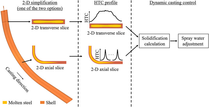
FIGURE 1. The typical control scheme of continuous casting.

In the meantime, it remains challenge to acquire accurate HTC values under different operating conditions. It is well known that HTC is a localized parameter and its value varies throughout the secondary cooling region (Sengupta et al., 2005). HTC is sensitive to both nozzle configurations and casting operating conditions. Some of the most recognized parameters that affect HTC include nozzle type, spray water flow rate, spray angle, standoff distance, steel surface temperature, spray direction, and nozzle-to-nozzle distance. In practice, researchers have correlated HTC with the most important operating parameters such as casting speed and spray water flow rate though small scale hot plate experiment (Nozaki et al., 1978; Morales et al., 1990; Horsky et al., 2005; Blazek et al., 2013; Long et al., 2018). The most well-recognized correlation was developed by Nozaki (Nozaki et al., 1978) and is shown in Eq. 2. This equation takes both spray water flux and spray water temperature into account, since both parameters are essential to the spray cooling process and are relatively convenient to obtain through on-site measurements. Nozaki also acknowledges the differences between caster machines by adding a machine-depend calibration parameter, ${\alpha }_{\text{cal}}$. With the knowledge of specific nozzle arrangement, this coefficient can be easily tuned. Due to its simplicity and flexibility, this correlation has been extensively used since 1970s. Some of the latest HTC correlations are either a variation of the Nozaki’s correlation (Brimacombe et al., 1980; Hardin et al., 2000; Hardin et al., 2003; Meng and Thomas, 2003; Mosayebidorcheh and Gorji-Bandpy, 2017; Hardin and Beckermann, 2018) or an extension of this formula (Blazek et al., 2013).

$\text{HTC}=22500Q_{\text{water}}^{0.55}\left(1-0.0075T_{\text{spray}}\right)/{\alpha }_{\text{cal}}(2)$

On the other hand, other important casting parameters such as steel surface temperature, casting speed, and nozzle-to-nozzle distance are not included in Eq. 2. For example, steel surface temperature has been proven to affect droplet impingement heat transfer and local Leidenfrost temperature (Bernardin and Mudawar, 1999). Casting speed can alter the droplet residence time on the steel surface, thereby increasing or decreasing the amount of energy transferred. And heat transfer is noticeably increased under the spray overlapping area in short nozzle-to-nozzle distance. Thus, it is necessary to develop more comprehensive and general HTC correlations to include these phenomena. In addition, it is worth mentioning that the existing correlations were specially developed for a limited number of nozzles and operation conditions. Each casting condition requires at least one experiment to uniquely determine the coefficients in the correlation and the correlation might be inapplicable when changes in the casting process occur.

With the advance of High-performance Parallel Computing (HPC) technique, Computational Fluid Dynamic (CFD)-based numerical models have become a powerful tool to gain insights into complex fluid flow and heat transfer problems. The major advantage of the HPC-powered CFD approach is to produce simulations on a massive scale within a reasonable short period of time. It is much more efficient to develop HTC correlations from numerical simulations. Yet, CFD-based HTC correlations for continuous casting are still not available, mostly owing to the complicated aerodynamic behaviors in atomization and the subsequent impingement heat transfer between water droplets and the hot steel. An accurate CFD model of the spray cooling process plays a pivotal role in developing reliable HTC correlations.

Therefore, the current study proposes a new efficient methodology to numerically develop HTC correlations for continuous casting of steel. The methodology includes high-fidelity three-dimensional CFD simulations of spray cooling with the consideration of atomization and impingement heat transfer and regression analysis. The CFD simulations predict detailed spray cooling effect on the steel surface under different operating conditions, whereas the regression analysis converts the simulation results into a mathematically simple correlation, which can be used as boundary condition for on-site off-line/on-line solidification calculation. In addition, a Graphic User Interface (GUI) was developed to facilitate the use of the correlation. The methodology presented in the current study should benefit the steel industry by expediting the development process of HTC correlations, achieving real-time dynamic spray cooling control, supporting nozzle selection, troubleshooting malfunctioning nozzles, and can further improve the accuracy of the existing casting control systems.

Methodology

Numerical Approach

Figure 2 illustrates the development process of HTC correlations using the numerical approach. The approach consists of numerical simulation stage, data analysis stage, and GUI development stage. CFD model development is the first step in the numerical simulation stage. The model contains the most important physics during spray cooling process, such as atomization, droplet breakup, droplet collision, air entrainment, droplet-steel impingement heat transfer, and steel slab cooling. The second step is to build a HTC database through parametric study. Different nozzle configurations and casting operating conditions are modeled in this step. In the data analysis stage, the distributions of different HTC profiles on steel surface are decomposed into two normalized universal distribution functions, whereas the magnitude of HTC is lumped into a characteristic value, which is correlated with eight representative operating parameters through regression analysis or curve fitting. Finally, a user-friendly graphic interface based on Unity® 3D platform computes the local HTC values based on the pre-defined correlation and the user inputs.

FIGURE 2

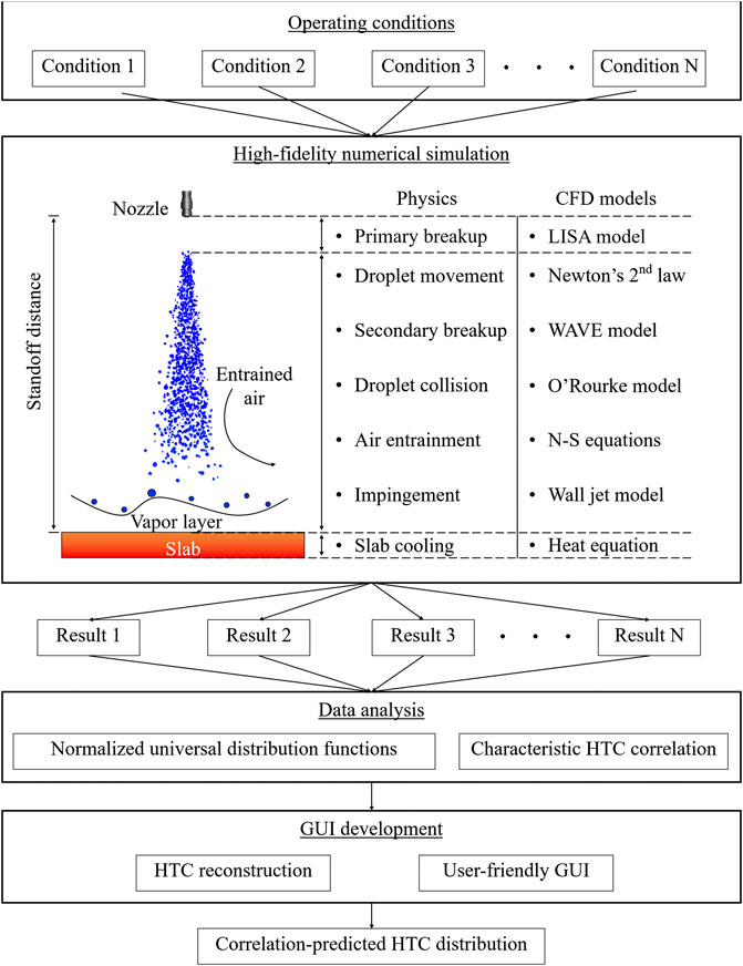
FIGURE 2. CFD-based development process of HTC correlation.

Numerical Models

The numerical simulation focuses on the atomization and droplet-steel impingement heat transfer. The breakup of water jet is not included in the current model but the resulting droplets from jet breakup are tracked in the Lagrangian frame from the breakup length to the end of their lifetime. Droplet motion is solved by integrating Newton’s second law. Air entrainment due to the high-speed water injection and hot steel slab are modeled as continuous phases in the Eulerian frame.

Continuous Phase

The steady state Reynolds-averaged Navier-Stokes equations for mass, momentum, energy, and species transport (water droplet to water vapor) are solved for air, whereas only the energy equation is required for steel slab to account for heat conduction, convection, and radiation. These conservation equations can be expressed in the following general form (Mundo et al., 1997; Liu et al., 2018):

$\nabla \cdot \left({\rho }_{\text{air}}{\overrightarrow{u}}_{\text{air}}\phi -{\text{Γ}}_{\phi }\nabla \phi \right)=S_{\phi }+S_{\text{drop}-\text{air}}(3)$

where $\phi$ is a universal variable and it represents one in mass equation, velocity in momentum equation, enthalpy in energy equation, and mass fraction in species transport equation. $S_{\phi }$ is the internal source term corresponding to the universal variable. $S_{\text{drop}-\text{air}}$ is the external source term that accounts for droplet-air interaction. The governing equations for air are solved first followed by unsteady droplet tracking. The air velocity in each computational cell is used to obtain droplet motion when integrating Newton’s law of motion. At the end of each droplet time step, the changes of mass, momentum, and energy in droplets are incorporated into the subsequent calculations for air through the external source term.

The k-ω Shear Stress Transport (SST) turbulence model solves for turbulence kinetic energy and specific turbulence dissipation rate. This model is chosen due to its high accuracy in predicting the presence of vortices along the spray boundary and the flow separation on the steel surface without consuming too much computational power. The model takes the advantage of the k-ε model in the bulk region and the k-ω model in the vicinity of walls with a blending function to transit between the two models (Menter, 1993; Zukerman and Lior, 2006).

Discrete Phase

Droplet Formation

Physically, droplets are formed through two sequential breakup processes, i.e., breakup of liquid sheet and breakup of ligaments. The two breakup processes are collectively referred to as primary breakup as opposed to secondary breakup where droplets formed from the primary breakup process further breakup into smaller droplets due to aerodynamic instabilities or droplet-droplet collisions. The primary breakup is a well-studied process and the corresponding theories have been rigorously validated in the past few decades (Rayleigh, 1878; Weber, 1931; Ohnesorge, 1936; Reitz, 1978a; Reitz, 1987b; Nijdam et al., 2006; Fung et al., 2012). The current study utilizes LISA model to predict droplet formation at the breakup length without modeling the internal flow inside the nozzle and the primary breakup process.

Figure 3 illustrates the droplet formation and injection process applied in the current study. The LISA model (O’Rourke, 1981; Senecal et al., 1999) assumes the liquid jet issued from nozzle as a two-dimensional viscous incompressible liquid sheet which breaks into ligaments and then droplets due to the growth of infinitesimal wavy disturbances after traveling a certain distance (breakup length) from nozzle exit. The breakup length is determined by the most unstable disturbance and its growth rate:

$L_b=\frac{U}{\Omega }\ln \left(\frac{{\eta }_b}{{\eta }_0}\right)(4)$

FIGURE 3

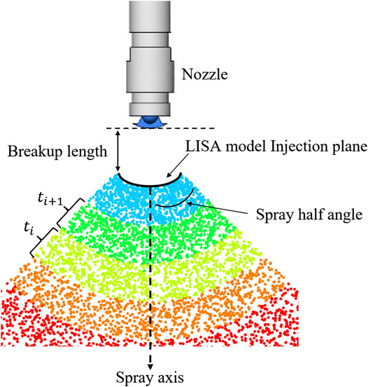
FIGURE 3. Droplet generation method by LISA model.

At the beginning of each droplet time step, $t_i$, a group of droplets are introduced into the computational domain from a virtual curved injection plane located at the distance of breakup length below the nozzle exit. The total mass of the introduced droplets is equal to the mass of water through the nozzle, which can be found from casting operating condition. Droplets are randomly distributed on the injection plane but their size distribution satisfies Rosin-Rammler distribution with a spread number of 3.5. The characteristic diameter of the Rosin-Rammler distribution can be computed from the following expression:

$d_0=3.76\frac{\pi C_L}{K_s}{\left(1+3\text{Oh}\right)}^{1/6}(5)$

Droplet Motion

Droplet motion within each droplet time step is tracked in the Lagrangian frame by solving Newton’s law of motion:

$\frac{d{\overrightarrow{u}}_{\text{drop}}}{dt}=\frac{3{\mu }_{\text{drop}}{C}_{D}R{e}_{\text{drop}}}{4{\rho }_{\text{drop}}{d}_{\text{drop}}^2}\left({\overrightarrow{u}}_{\text{air}}-{\overrightarrow{u}}_{\text{drop}}\right)+\frac{\overrightarrow{g}\left({\rho }_{\text{drop}}-{\rho }_{\text{air}}\right)}{{\rho }_{\text{drop}}}(6)$

Droplet motion is governed by drag force and gravitational force simultaneously with the assumption that droplet remains spherical throughout its lifetime. The drag force term represents the air-droplet interaction and the drag coefficient, $C_D$, can be found from the following piecewise function (Liu et al., 1993):

$C_D=\{\begin{array}{cc}\begin{array}{c}0.424\\ \frac{24}{R{e}_{\text{drop}}}\left(1+\frac{1}{6}{\text{Re}}_{\text{drop}}^{2/3}\right)\end{array}& \begin{array}{c}{\text{Re}}_{\text{drop}}>1000\\ {\text{Re}}_{\text{drop}}\le 1000\end{array}\end{array}(7)$

The eddy-lifetime model is also incorporated to simulate the dispersion of droplets during atomization due to turbulence in the gas phase (Gosman and Ioannides, 1983).

Droplet Temperature and Mass Change

Droplet also exchanges heat with the surrounding air while traveling through the gas phase. The temperature change of a droplet is determined by the conservation of energy:

$m_{\text{drop}}{c}_p\frac{d{T}_{\text{drop}}}{dt}=\pi d_{\text{drop}}^{2}h\left(T_{\infty }-T_{\text{drop}}\right)+\frac{d{m}_{\text{drop}}}{dt}{h}_{fg}+\pi d_{\text{drop}}^2{\epsilon }_{\text{drop}}{\sigma }_{SB}\left(T_R^4-T_{\text{drop}}^4\right)(8)$

The convective heat transfer coefficient, $h$, can be obtained from the Ranz-Marshall model (Ranz and Marshall, 1952):

${\text{Nu}}_{\text{drop}}=\frac{{\mathit{hd}}_{\text{drop}}}{k_{\text{air}}}=2.0+0.6{\mathrm{Re}}_{\text{drop}}^{0.5}{\mathrm{Pr}}^{0.33}(9)$

In the meantime, liquid droplet vaporizes into water vapor which then diffuses into the surrounding gas phase as long as a concentration difference exists between droplet surface and the bulk fluid. This process is simulated by constantly updating droplet mass in each droplet time step:

$\frac{d{m}_{\text{drop}}}{dt}=\pi d_{\text{drop}}^2{k}_c\left(C_s-C_{\infty }\right)(10)$

The mass transfer coefficient, $k_c$, can be obtained from the following Sherwood number correlation:

${\text{Sh}}_{\text{drop}}=\frac{k_c{d}_{\text{drop}}}{D_{\text{vapor}}}=2.0+0.6{\text{Re}}_{\text{drop}}^{0.5}{\text{Sc}}^{0.33}(11)$

Droplet Breakup and Collision

Droplet breakup and collision predictions are crucial for the subsequent droplet-steel impingement heat transfer. Droplet numbers and size undergo significant changes during these two events. The WAVE breakup model is applied in the current study to account for the breakup of droplets induced by the relative velocity between droplet and the surrounding air. The model is an analogy to the jet instability theory. The model assumes that the breakup time of a droplet and the resulting child droplet size depend on the fastest-growing Kelvin-Helmholtz instability:

$r_{\text{child}}=B_0\Lambda (12)$

$\frac{d{r}_{\text{parent}}}{dt}=-\frac{\Lambda \Omega \left(r_{\text{parent}}-r_{\text{child}}\right)}{3.726B_1{r}_{\text{parent}}}(13)$

Droplet-droplet collision is calculated by O’Rourke’s algorithm (O’Rourke, 1981). The algorithm gives a stochastic estimation of collisions instead of calculating whether or not the trajectories of two droplets intersect. At each droplet time step, droplets are considered to be able to collide only if they present at the same computational cell and the smaller droplet is within the collision volume centered at the larger one. The collision volume is defined as a cylinder with a length of $\left(u_1-u_2\right)\Delta t$ and a circular area of $\pi {\left(r_1+r_2\right)}^2$. If the condition is satisfied, the two droplets are subject to collide. According to the concept of collision volume, the probability of collision can be defined as follows:

$P\left(n\right)=e^{-\overline{n}}\frac{{\overline{n}}^n}{n!}(14)$

$\overline{n}=\frac{n_2\pi {\left(r_1+r_2\right)}^2\left(u_1-u_2\right)\Delta t}{V_{\text{cell}}}(15)$

The outcome of a collision depends on the offset of the trajectory of the smaller droplet to the larger droplet. The offset is a function of the center distance between the two droplets and a random number, which resembles the randomness of collisions:

$b_{\text{offset}}=\left(r_1+r_2\right)\sqrt{P}(16)$

The calculated offset is compared with a critical value defined as follows:

$b_{\text{crit}}=\left(r_1+r_2\right)\sqrt{\min \left(1.0,\frac{2.4f}{\text{We}}\right)}(17)$

$f={\left(\frac{r_1}{r_2}\right)}^3-2.4{\left(\frac{r_1}{r_2}\right)}^2+2.7\left(\frac{r_1}{r_2}\right)(18)$

If $b_{\text{offset}}<b_{\text{crit}}$, the outcome of the collision is coalescence, otherwise the two droplets bounce off from each other. The magnitude and direction of droplet velocities after the collision is computed from the conservation of kinetic energy and momentum.

Droplet-Steel Impingement Heat Transfer

Figure 4 illustrates the calculation of droplet-steel impingement and heat transfer. A fluid cell, a solid cell, as well as a water droplet are depicted in the figure. When a droplet enters a fluid cell adjacent to a solid cell and impinges on the fluid-solid interface, the outcome of the impingement depends on the properties of the incoming droplet and is calculated by the wall jet model (Naber and Reitz, 1988). There are three outcomes included in the impingement model, i.e., deposit, reflection, and wall jet. In the deposit mode, droplet stays on the steel surface after impingement and continues to extract heat from steel until it completely evaporates. In the reflection mode, the vertical component of droplet velocity prior to impingement is changed to opposite sign after impingement while maintaining the magnitude. Both direction and magnitude of the tangent velocity component remains the same.

FIGURE 4

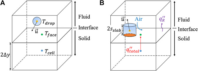
FIGURE 4. Droplet-steel impingement heat transfer calculation (A) before impingement, and (B) after impingement.

The wall jet mode, however, is activated when a group of closely-spaced droplets impinges on the steel surface. This continuous stream of droplets loses vertical velocity component and turns to horizontal direction after impingement, which can be treated as an inviscid jet emitted from the stagnation point on the surface. As illustrated in Figure 5, the height of the wall jet, $\mathit{H}$, is a function of the angle at which droplet leaves the horizontal impingement:

$H\left(\Psi \right)=H_{\pi }{e}^{\beta \left(1-\frac{\text{Ψ}}{\pi }\right)}(19)$

Where $H_{\pi }$ is the height at $\Psi =\pi$. The constant, $\beta$, is determined from the conservation of mass and momentum and is given by Naber and Reitz (Naber and Reitz, 1988):

$\sin \left(\varphi \right)=\frac{e^{\beta }+1}{\left(e^{\beta }-1\right)\left[1+{\left(\frac{\pi }{\beta }\right)}^2\right]}(20)$

FIGURE 5

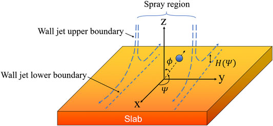
FIGURE 5. Illustration of wall-jet impingement mode.

Droplet-steel heat transfer is illustrated in Figure 4B. Although droplet is assumed to be spherical throughout its lifetime, the effect of droplet deformation is taken into account in the heat transfer calculation. The current study assumes that droplet deforms into an equal-volume cylinder upon impingement and remains in contact with the hot surface for a short period of time. The deformed droplet and steel exchange heat through pure conduction:

$\frac{d}{dt}\left(m_{\text{drop}}{c}_p{T}_{\text{drop}}\right)=\frac{k_{\text{drop}}{A}_{\text{cond}}}{s_{\text{slab}}}\left(T_{\text{face}}-T_{\text{drop}}\right)(21)$

The effective contact area, $A_{\text{cond}}$, and the contact time are defined as follows (Akao et al., 1980; Birkhold, 2007):

$A_{\text{cond}}=\frac{\pi }{8}{\left(0.61d_{\text{drop}}W{e}^{0.38}\right)}^2(22)$

$t_{\text{drop}}=\frac{\pi }{10}\sqrt{\frac{{\rho }_{\text{drop}}{d}_{\text{drop}}^3}{\sigma }}(23)$

Another important phenomenon during spray cooling is the Leidenfrost effect. It takes place when steel surface temperature is above the Leidenfrost temperature. In this situation, liquid droplet evaporates into vapor immediately after impingement. Due to the low thermal conductivity, vapor hovering above the surface acts as an insulation layer, preventing further contact between liquid droplet and the hot surface. It is worth mentioning that the steel surface temperature is generally higher than the Leidenfrost temperature throughout continuous casting process (Bernardin and Mudawar, 1999). Thus, a coefficient, i.e., heat transfer effectiveness, is incorporated in the impingement heat transfer model to account for the reduction in heat flux through the steel surface due to the existence of vapor layer. The coefficient is the ratio of actual heat flux and the maximum heat flux that can be achieved. An experiment-based empirical correlation is applied to calculate the coefficient (Issa, 2004):

$\text{eff}=3.771\times {10}^{-3}{\text{We}}^{0.691}\text{exp}\left(-9.079\times {10}^{-4}\text{We}\right)(24)$

Heat Transfer Coefficient Calculation

HTC is evaluated in post-processing after the simulation is completed. In practice, it is convenient to combine both conduction and convection into one single term and represent this amount of heat transfer by Newton’s law of cooling. Based on Eq. 1 and Figure 4 with the consideration of energy conservation, the total heat flux that is transferred from the centroid of the solid cell to the centroid of the fluid-solid interface can be written as follows:

$q_{\text{total}}^{″}=\frac{{\lambda }_{\text{steel}}\left(T_{\text{cell}}-T_{\text{face}}\right)}{\text{Δ}y}=\text{HTC}\left(T_{\text{face}}-T_{\text{drop}}\right)+q_R^{″}(25)$

Where $T_{\text{cell}}$ is the temperature of the solid centroid, $T_{\text{face}}$ is the temperature of the interface centroid, $\text{Δ}y$ is the distance from the solid centroid to the face centroid and is equal to half of the cell height, $T_{\text{drop}}$ is the temperature of droplet upon impingement. However, it is not feasible to measure the temperature of each induvial droplet before and after impingement in reality. A more practical method adopted by the steel industry is to replace term with the spray water temperature, which is measurable and controllable. The current study also adopts this definition in order to produce consistent HTC values. Rearranging Eq. 25 and solving for HTC, yield the following expression:

$\text{HTC}=\frac{{\lambda }_{\text{steel}}\left(T_{\text{cell}}-T_{\text{face}}\right)-\text{Δ}y{q}_R^{″}}{\text{Δ}y\left(T_{\text{face}}-T_{\text{drop}}\right)}(26)$

Computational Domain and Boundary Conditions

In continuous casting process, the secondary cooling region extends from the mold exit to the cut-off point and the total length of this region is between 10 and 40 m. Besides, hundreds of alternating water sprays and rolls are placed on both broad faces of the steel strand. On the other hand, the average size of a liquid droplet is only around 300 μm and the computational cells in CFD simulations must have a comparable size in order to resolve detailed droplet-air interaction, droplet-droplet interaction, and droplet-steel interaction. Therefore, a more efficient way to model the spray cooling process is to simulate a small portion of the entire caster machine. Figure 6 demonstrates the computational domain applied in the current study. The domain contains only one spray and a 30 mm-thick solid steel segment. In practice, the nozzle type, spray angle, water flow rate, spray standoff distance, and nozzle-to-nozzle distance are different from spray to spray, but the current computational domain can be used to simulate different sprays with minor changes of boundary conditions.

FIGURE 6

FIGURE 6. Computational domain and boundary conditions for spray cooling simulation.

Droplet injection, breakup, collision, impingement, and evaporation are solved in the fluid region, whereas heat conduction inside the steel slab is computed in the solid region. The average thickness of the solidified shell is between 25 and 30 mm at the mold exit and the growth rate of the shell is estimated between 0.1 mm/s and 0.4 mm/s (Tang et al., 2012). Thus, the 30 mm-thick slab applied in the current study is thick enough to include the temperature gradient within the solid steel slab but thin enough to exclude solidification within the steel slab. At the normal casting speed of 1 m/min, it takes 6 s for the steel slab to pass a spray which spans 100  mm in the casting direction, but it only takes 0.01 s for droplets traveling at 13 m/s to reach the steel surface which is placed 130 mm below the nozzle tip. Due to the drastic difference in time scale, it is numerically convenient and efficient to exclude the solidification process from the current simulations.

All of the surfaces of the fluid region are set as pressure outlets except the interface, as shown in Figure 6. Thermal conditions on the interface are determined through conjugate heat transfer. The two side surfaces of the solid region that are parallel to the casting direction are treated as symmetric planes with the assumption that heat conduction through these surfaces are negligible. Temperature distribution on the upstream surface is assumed to satisfy linear distribution owing to the fact that the simulated solid region is only a small fraction of the entire steel slab (Koric and Thomas, 2006). The lower and upper limits of the temperature distribution are obtained from plane historic data. A fixed temperature is assigned to the bottom surface and its magnitude is set to the maximum temperature on the upstream surface to ensure the consistence of the boundary conditions. The initial temperature of the face centroid on the downstream surface of the solid region is set to that of the closest cell centroid. The temperature of the face centroid is constantly updating during the simulation according to the upstream conditions. In addition, a moving reference frame is applied to the solid region to represent the movement of steel slab in the real process.

An uneven-spaced hexahedral-based mesh is applied in both fluid and solid regions. Mesh cells are biased toward the center of the spray and the fluid-solid interface to ensure the non-dimensional wall distance, $y^{+}$, is less than one in the vicinity of the interface. All of the simulations were conducted on the platform of ANSYS Fluent 17.1. A transient droplet tracking is performed after two hundred iterations for the continuous phases. Convergence is considered to be satisfied once all of the scaled residuals reach to 10^–6.

Operating Conditions

Eight operating parameters are identified as contributing factors to determining HTC values and they are spray water flow rate, nozzle-to-nozzle distance, standoff distance, spray water temperature, casting speed, distance between adjacent spray rows, spray angle, and spray direction. Table 1 summaries all of the contributing factors and their corresponding ranges applied in the current study. It is noteworthy that the unit of each factor is converted in accordance with the plant operation. Furthermore, slab surface temperature is excluded from the parametric study for two reasons: 1) slab surface temperature is above the Leidenfrost temperature (700°C–1,000°C) in continuous casting of steel. Under such condition, heat extraction during spray cooling is dominated by vapor film boiling mechanism. The change of HTC with slab surface temperature is negligible (Sengupta et al., 2005). 2) slab surface temperature is one of the to-be-determined parameters during solidification calculation, which depends on HTC as the thermal boundary condition.

TABLE 1

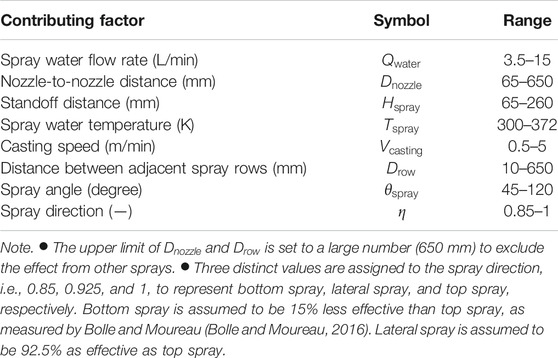
TABLE 1. Summary of contributing factors applied in the current study.

Validation

Droplet Size

Droplet size prediction prior to the impingement is crucial for determining the impingement outcome and the corresponding heat transfer rate. The droplet size distribution of a Lechler 660.766 flat-fan spray nozzle (1.9 mm equivalent orifice diameter and 90° spray angle) was experimentally measured by an industrial collaborator. The nozzle was placed 130 mm away from the measurement plane. Liquid water was injected at the rate of three gallon per minute (11.36 L per minute) under isothermal condition. The VisiSize laser imaging system was adopted to measure the droplet size.

The measured average diameter from 0 mm (spray center) to 120 mm (spray edge) with the increment of 20 mm were compared with the simulation and the result is shown in Figure 7. The predicted droplet size shows good agreements with the measured data. Droplet size is much smaller in the core of the spray where droplet concentration is the highest, mostly due to intense breakup and collisions. A good match of droplet size in this region suggests that the current model is able to accurately capture the most important phenomena inside a spray. The predictions near the edge of the spray where droplet-air interaction prevails are slightly off. One of the possible reasons is that the strong interaction between the two phases introduces other types of breakup which are not included in the current model. Nonetheless, the majority of the sprays in continuous casting are designed to overlap with the adjacent sprays and the effect of droplet-air interaction is significantly reduced in the overlapping area.

FIGURE 7

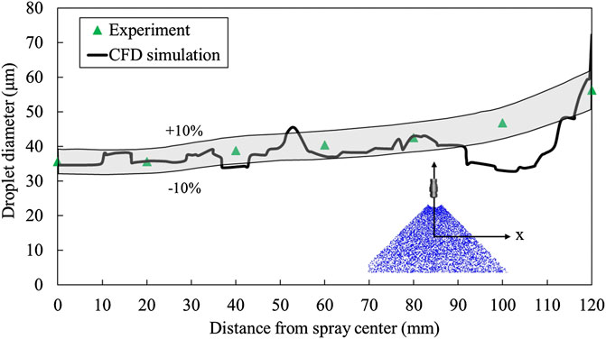
FIGURE 7. Comparison of droplet size at different locations within a spray.

Impingement Heat Transfer

The impingement heat transfer model was validated against the hot plate experiment conducted at Brno University of Technology (Horsky et al., 2005). A segment of an austenitic plate was heated up to 1,250°C prior to the experiment. All of the surfaces of the hot plate were covered with insulation materials except the surface facing the spray nozzle. The plate was fixed above the nozzle to eliminate the generation of water film on the surface. The nozzle was placed on a moving trolly which can move back and forth during the experiment to mimic the relative movement between the steel slab and the sprays in continuous casting. The experiment stopped when the plate temperature was below 500°C. A set of thermocouples embedded in the plate recorded the inner temperatures and the surface HTC were calculated by the inverse heat transfer method.

Figure 8 shows the comparison of integrated surface HTCs at different locations on the surface, together with the overall HTC. The predicted HTC values are in agreement with majority of the measurements. The large HTC values at location A and B indicate intense spray cooling. This is because a large number of small droplets with large surface to volume ratio significantly promote heat transfer in the center of the spray. A few outliers imply that the current model underpredicts the heat transfer at some locations on the surface. One possible reason is related to the experiment procedure. The transient hot plate method is designed to run through a wide temperature range in one experiment. As a result, the plate temperature might drop below the Leidenfrost temperature at the end of the experiment. At low surface temperatures, liquid droplets are able to directly contact with the plate and result in much higher HTCs. Without considering spray cooling under the Leidenfrost temperature, the current model is able to predict accurate HTC values.

FIGURE 8

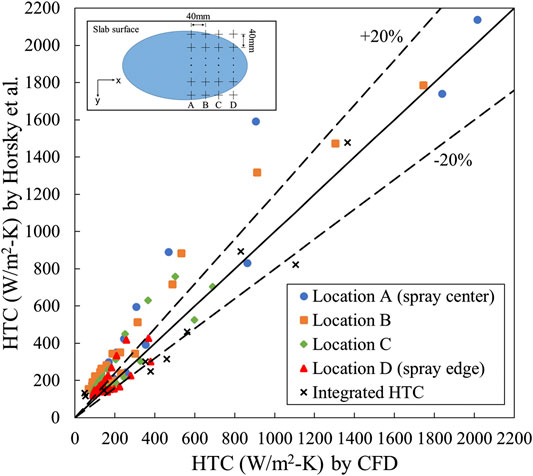
FIGURE 8. Comparison of HTC on the steel surface.

Results and Discussions

Heat Transfer Coefficient Distribution on Steel Surface

Figure 9 shows the temperature and HTC distributions on the steel surface cooled by a single flat-fan nozzle at a typical casting condition: $Q_{\text{water}}$ = 7 L/min, $D_{\text{nozzle}}$ = $D_{\text{row}}$ = 650 mm, $H_{\text{spray}}$ = 130 mm, $T_{\text{spray}}$ = 300 K, $V_{\text{casting}}$ = 1 m/min, ${\theta }_{\text{spray}}$ = 90°, $\eta$ = 1. The low temperature spray cooling region in the middle is narrow in the casting direction but stretches almost 200 mm in the transverse direction, forming a visible elliptic pattern on the surface. The fact that the impingement heat transfer pattern aligns with the flat-fan spray pattern reveals the dominant effect of spray characteristics on spray cooling. Outside the spray cooling region, the steel slab loses heat to the environment through convection and radiation. The nearly symmetric elliptic pattern also indicates the droplet distribution on the surface. After impingement, the majority of droplets split into two streams and continue to move in the transverse direction. The two streams depart from each other at the stagnation point about which the elliptic pattern is symmetric.

FIGURE 9

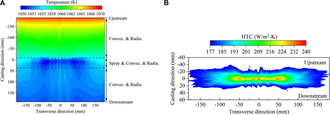
FIGURE 9. (A) top view of slab surface temperature, and (B) top view of HTC pattern.

Figure 9B shows the HTC profile on the surface. The local HTC values are computed based on Eq. 26. Within the butterfly-shaped profile, HTC peaks near the stagnation point where droplet momentum is the highest. According to Eq. 24, heat transfer effectiveness increases with the increase of droplet Weber number. As a result, high-momentum droplets produce higher HTC values upon impingement. Such behavior implies that droplets with high momentum are more likely to penetrate the thin vapor layer hovering above the steel surface and make direct contact with the surface.

Other operating conditions produce similar HTC profiles on the steel surface but with some variations in magnitude. Since all of the CFD-predicted HTC profiles have similar distributions in space, it is much more convenient to create normalized universal distribution functions for all of the operating conditions. The HTC distribution on the steel surface can be decomposed into two universal distribution functions. One is in the casting direction (y direction) and another is in the transverse direction (x direction). The coordinates, together with the corresponding HTC value, at any given point in a CFD-predicted HTC profile are normalized to values between 0 and one based on the following definitions:

$X_{\text{norm},i}=\frac{X_i-\min \left(X_1, X_2,\dots ,X_n\right)}{\max \left(X_1, X_2,\dots ,X_n\right)-\min \left(X_1, X_2,\dots ,X_n\right)}(27)$

${\text{HTC}}_{\text{norm}-x,i}=\frac{{\text{HTC}}_i-\text{min}\left({\text{HTC}}_1,{\text{ HTC}}_2,\dots ,{\text{HTC}}_n\right)}{\max \left({\text{HTC}}_1,{\text{ HTC}}_2,\dots ,{\text{HTC}}_n\right)-\text{min}\left({\text{HTC}}_1,{\text{ HTC}}_2,\dots ,{\text{HTC}}_n\right)}(28)$

$Y_{\text{norm},j}=\frac{Y_j-\min \left(Y_1, Y_2,\dots ,Y_m\right)}{\max \left(Y_1, Y_2,\dots ,Y_m\right)-\min \left(Y_1, Y_2,\dots ,Y_m\right)}(29)$

${\text{HTC}}_{\text{norm}-y,j}=\frac{{\text{HTC}}_j-\text{min}\left({\text{HTC}}_1, {\text{HTC}}_2,\dots ,{\text{HTC}}_m\right)}{\max \left({\text{HTC}}_1,{\text{ HTC}}_2,\dots ,{\text{HTC}}_m\right)-\text{min}\left({\text{HTC}}_1,{\text{ HTC}}_2,\dots ,{\text{HTC}}_m\right)}(30)$

Figure 10 illustrates the shape and location of the two normalized HTC distributions. The two distributions can be treated as the projections of the two-dimensional HTC pattern. The outline of the two normalized universal distribution functions can be obtained through curve fitting and are expressed as follows:

$\begin{array}{c}f\left(X_{\text{norm}}\right)=-0.3292\exp \left[-{\left(\frac{X_{\text{norm}}-0.09755}{0.1308}\right)}^2\right]+0.09584\exp \\ \left[-{\left(\frac{X_{\text{norm}}-0.5738}{0.1081}\right)}^2\right]-426.2\exp \left[-{\left(\frac{X_{\text{norm}}-229.1}{100.3}\right)}^2\right]+3.342\exp \\ \left[-{\left(\frac{X_{\text{norm}}-0.4192}{0.7977}\right)}^2\right]+0.1656\exp \left[-{\left(\frac{X_{\text{norm}}-0.7374}{0.1038}\right)}^2\right]+0.7229\exp \left[-{\left(\frac{X_{\text{norm}}-1.232}{0.3436}\right)}^2\right]\end{array}(31)$

$\begin{array}{c}f\left(Y_{\text{norm}}\right)=0.2583\exp \left[-{\left(\frac{Y_{\text{norm}}-0.4542}{0.1822}\right)}^2\right]+91.13\exp \\ \left[-{\left(\frac{Y_{\text{norm}}-0.6977}{0.1257}\right)}^2\right]-0.142\exp \\ \left[-{\left(\frac{Y_{\text{norm}}-0.6394}{0.03364}\right)}^2\right]-90.58\exp \\ \left[-{\left(\frac{Y_{\text{norm}}-0.6983}{0.1252}\right)}^2\right]\end{array}(32)$

FIGURE 10

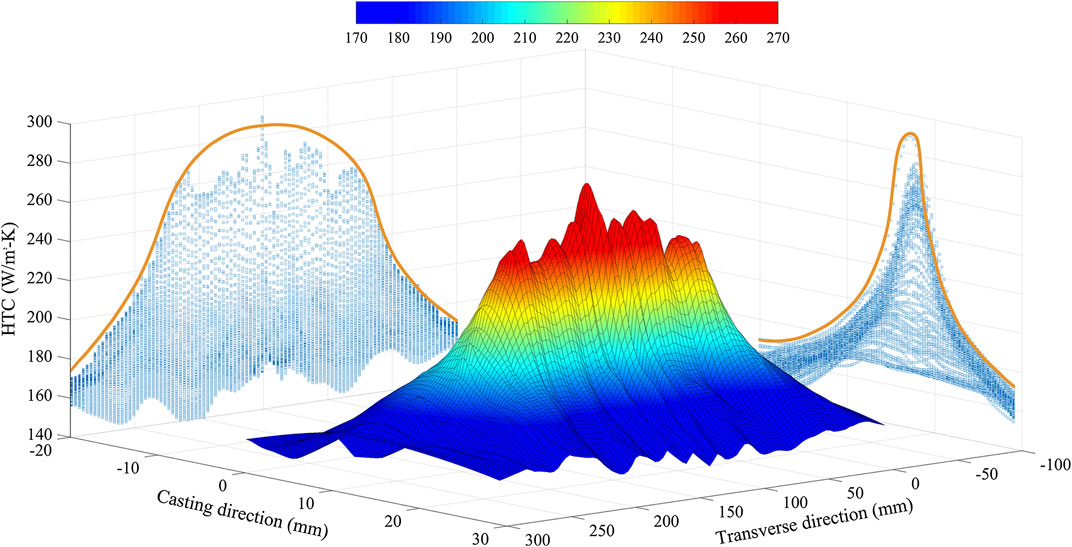
FIGURE 10. Illustration of the two projected universal HTC distributions.

Heat Transfer Coefficient Correlation

HTC correlation can be seen as a form of reduced-order model. In the field of heat transfer, HTC correlations are usually expressed in non-dimensional forms in order to reveal the governing physical parameters explicitly. While the non-dimensional correlations are widely adopted by academia, they are somewhat obscure for casting operations. In practice, HTC is expressed in dimensional forms and is a function of measurable operating parameters. The current study follows this convention and all of the correlations are expressed in dimensional forms.

HTC is a localized parameter and its value varies in both casting direction and transvers direction, as shown in Figure 9B. However, with the assumption that the HTC distributions from different operating conditions satisfy the same normalized universal distribution function in the same direction, the HTC distribution under any given operating condition can be reconstructed based on the two universal distribution functions defined in Eqs 31 and 32 and an operating condition-dependent characteristic HTC. Such characteristic HTC is independent of special coordinates and it is a unique lumped value for a specific condition. The current study utilizes the maximum HTC within the HTC profile as the characteristic value.

The correlation between the characteristic HTC and the eight operating parameters can be obtained through either linear regression analysis or curve fitting. However, the final form of the correlation should be mathematically simple otherwise it will require a significant amount of computational time which results in delaying the casting control. The most straightforward correlation is to assume that the characteristic HTC, or lumped HTC, is an explicit linear function of the operating parameters:

${\text{HTC}}_{\text{lump}}=A_0+A_1{Q}_{\text{water}}+A_2{D}_{\text{nozzle}}+A_3{H}_{\text{spray}}+A_4{T}_{\text{spray}}+A_5{V}_{\text{casting}}+A_6{D}_{\text{row}}+A_7{\theta }_{\text{spray}}+A_8\eta (33)$

The coefficients in Eq. 33 can be found through multivariable linear regression analysis. The current study adopted OriginLab® to obtain the coefficients and the final form of the multivariable linear regression-based correlation is shown as follows:

$\begin{array}{c}{\text{HTC}}_{\text{lump}}=111.718+14.856Q_{\text{water}}+0.01325D_{\text{nozzle}}-0.126H_{\text{spray}}\\ -0.255T_{\text{spray}}+39.218V_{\text{casting}}+0.0415D_{\text{row}}\\ -0.853{\theta }_{\text{spray}}+196.568\eta , R^2\\ =0.639\end{array}(34)$

Alternatively, it is mathematically convenient to combine all eight operating parameters into a single variable and convert the multivariable linear regression analysis to single variable linear regression analysis. The combined single variable can be written as follows:

$\chi =b_1{Q}_{\text{water}}^{a_1}{b}_2{D}_{\text{nozzle}}^{a_2}{b}_3{H}_{\text{spray}}^{a_3}{b}_4{T}_{\text{spray}}^{a_4}{b}_5{V}_{\text{casting}}^{a_5}{b}_6{D}_{\text{row}}^{a_6}{b}_7{\theta }_{\text{spray}}^{a_7}{b}_8{\eta }^{a_8}(35)$

Coefficients in Eq. 35 are not uniquely determined. They can be regarded as the weight of each operating parameter and can be calibrated for different caster machines. The coefficients applied in the current study are based on an industrial collaborator’s caster machine and the calibrated single variable is as follows:

$\chi =57.408Q_{\text{water}}^{0.03}{D}_{\text{nozzle}}^{0.03}{H}_{\text{spray}}^{0.05}{T}_{\text{spray}}^{0.06}100V_{\text{casting}}^{0.06}{D}_{\text{row}}^{0.05}{\theta }_{\text{spray}}^{0.01}1.265{\eta }^{0.06}(36)$

The combined variable $\chi$ is correlated with the lumped HTC through both linear regression analysis and exponential curve fitting in the current study. The two correlations are shown as follows:

${\text{HTC}}_{\text{lump}}=-235.018+1.783\chi , R^2=0.248(37)$

${\text{HTC}}_{\text{lump}}=665.7\text{exp}\left(-0.003294\chi \right)+0.000005927\exp \left(0.05004\chi \right), R^2=0.507(38)$

Figure 11 shows the comparison between the CFD-predicted HTCs and the correlation-predicted HTCs. The multivariable linear correlation tends to overpredict heat transfer at lower values of HTC but underpredict spray cooling at higher values. The exponential correlation shows similar trends as well. The predictions from the single variable linear correlation are more accurate than the other two at lower values of HTC, then the predictions become oscillating between overpredicting and underpredicting at larger HTC values. Overall, the multivariable linear correlation is the best fit among all three correlations in terms of accuracy. Besides, it only involves two basic mathematic operations, i.e. multiplication and addition. Such features should allow fast prediction, thereby enabling real-time casting control. However, the other two correlations can still be considered as potential candidates. With careful calibration of the combined single variable, the more sophisticated mathematic operations in these two correlations can better reveal the intertwined nature between the casting operating parameters.

FIGURE 11

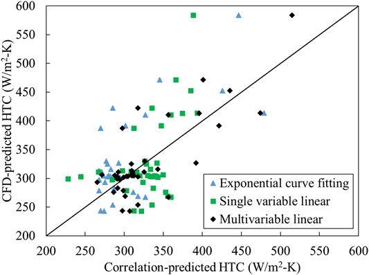
FIGURE 11. Comparison between the CFD-predicted HTCs and the correlation-predicted HTCs.

Heat Transfer Coefficient Reconstruction and GUI

The localized HTC distribution is reconstructed during the application. The reconstruction process consists of three stages, i.e., defining HTC coverage, computing lumped HTC, and generating HTC distribution. HTC coverage is excluded from the universal distribution functions, but it should be considered in the reconstruction stage. For any given operating condition, the HTC coverage on the steel surface can be calculated based on standoff distance, spray angle (on the plane that is perpendicular to the casting direction), and spread angle (on the plane that is perpendicular to the transverse direction), as shown in Figures 12A,B. The boundaries of the HTC coverage, as shown in Figure 12C, can be found from trigonometric relations and are defined as follows:

$X_{\min }=0, X_{\max }=2H_{\text{spray}}\tan \left(\frac{{\theta }_{\text{spray}}}{2}\right),Y_{\min }=0,Y_{\max }=2H_{\text{spray}}\tan \left(\frac{{\theta }_{\text{spread}}}{2}\right)(39)$

FIGURE 12

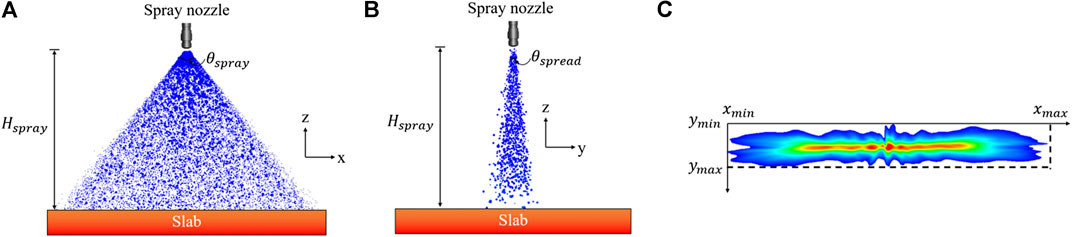
FIGURE 12. Calculation of HTC coverage on the steel surface (A) casting direction, (B) transverse direction, and (C) top view of HTC pattern.

The lumped HTC is calculated based on Eq. 34 with the eight pre-determined operating parameters. Finally, the local HTC value at any given point, ($X_i, Y_j$), within the HTC coverage can be computed based on Eqs 27, 29, 31, and 32:

${\text{HTC}}_{\text{local}}=f\left(X_{\text{norm}}\right)f\left(Y_{\text{norm}}\right){\text{HTC}}_{\text{lump}}(40)$

Repeating the aforementioned process with user-defined increments in both directions, a two-dimensional HTC distribution is generated. Figure 13 shows the comparison of CFD-predicted HTC distribution and correlation-predicted HTC distribution. The HTC distribution obtained from CFD simulation has random spikes across the coverage compared to the smooth distribution predicted by correlation. This is because the high-fidelity CFD simulation is able to capture detailed phenomena during droplet-steel impingement heat transfer, such as droplet reflection and sliding droplet on steel surface. The reconstructed low order HTC distribution excludes some of these detailed local effects to gain computational efficiency.

FIGURE 13

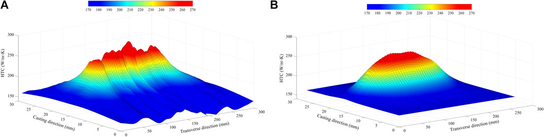
FIGURE 13. Comparison of HTC distributions (A) CFD-predicted, and (B) correlation-predicted.

The correlation along with the reconstruction procedure developed in the current study can be programmed in new casting control systems as a subroutine. Alternatively, a GUI was created as a complementary component for the existing control systems. Figure 14 shows the interface of the beta version. The interface illustrates the definition of HTC coverage to eliminate confusions and ambiguities. The input buttons allow users to type the values of the eight operating parameters and the increments in the two directions. An on-demand hidden window contains the detailed definition of each input parameter. The program executes when users click on the “Generate” button and creates a spreadsheet in versatile comma-separated values (csv) format, which includes the special coordinates and the corresponding local HTC values within the HTC coverage. The spreadsheet can be conveniently imported into the existing control system as the boundary condition for solidification calculation. Future versions of the HTC GUI will focus on producing massive HTC predictions by allowing users to import a matrix of operating conditions instead of typing the numbers manually.

FIGURE 14

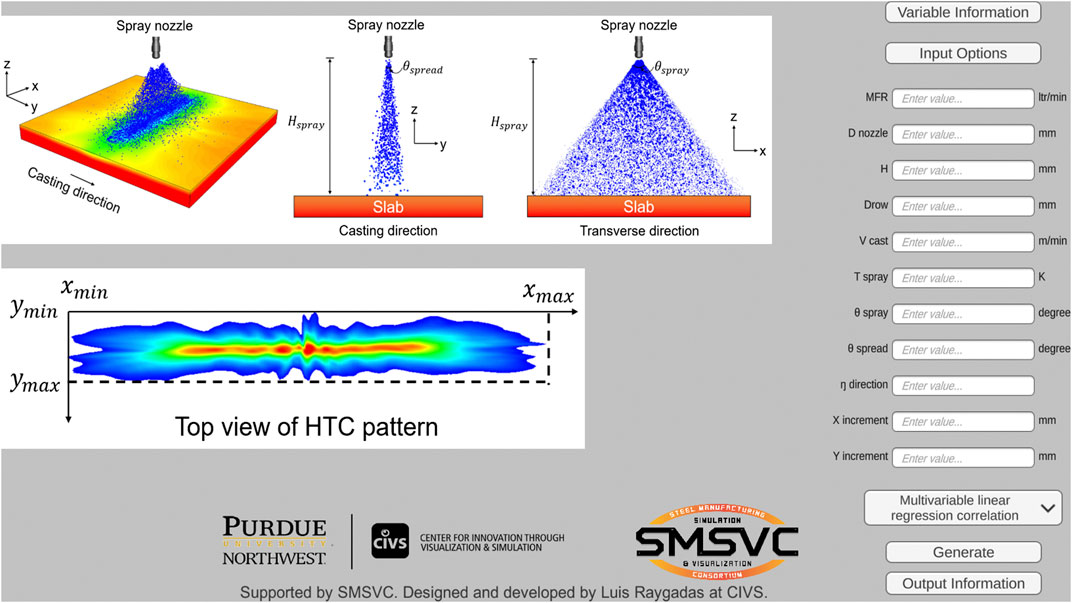
FIGURE 14. Graphic User Interface of HTC correlation.

Potential Applications

5 Aforementioned HTC correlations, together with the GUI, should benefit the steel industry from at least the following aspects: 1) accelerating the development process of HTC correlations for new nozzle configurations and operating conditions. For example, the spray cooling technology is consistently evolving as the nozzle manufactures advance spray nozzle designs. New spray characteristics, i.e., finer water droplet size, shorter liquid sheet breakup length, and multi-phase spray, etc., must be considered in HTC correlations. The current numerical approach should significantly reduce the amount of time to develop new correlations whenever spray characteristics change. Moreover, the demand for new types of steel products is increasing steadily. Each type of steel requires special spray cooling strategy, including nozzle type (hydraulic or air-mist), nozzle layout, and spray intensity (spray flow rate and standoff distance). The current high-performance computer-aided numerical method will be useful for designing new cooling strategy in a timely manner. 2) realizing on-site real-time dynamic spray cooling control. One of the primary goals of developing HTC correlations is to enable real-time control during continuous casting. The HTC correlations proposed in this study and the user-friendly interface will allow instant generation of HTC values on both casting and transverse directions. When this prediction process is automated and integrated with solidification prediction module and control module, the prediction and dynamic control process can be completed in near real-time. 3) supporting spray nozzle selection during caster design stage. The current HTC GUI was built for both off-line and on-line applications. When applied off-line, the HTC GUI can be used for “what if” scenarios and provide HTC values for different nozzle arrangements and operating conditions. Engineers can select the optimum nozzle type and cooling strategy for a specific caster based on the predicted HTC values. 4) Troubleshooting malfunctioning nozzles. The previous HTC correlations were developed based on ideal operating conditions. Thus, they can be used to identify nozzles that deviate from design conditions. For example, clogged nozzles due to inclusion deposition will produce different spray pattern on slab surface, therefore, generate different cooling profile. Operator can compare the predicted temperature profile with the measured one and pinpoint the malfunctioning nozzle where the temperature difference is large (beyond tolerance).

Conclusion

Efficient heat removal without compromising steel strength and quality during secondary cooling process requires accurate casting control and dynamic adjustment of spray water flow rate. In practice, HTC on steel surface has been adopted as an indicator to quantify the spray cooling rate and has also been served as one of the critical boundary conditions for solidification calculation. Experimental-based HTC correlations haven been widely used across the industry to predict HTC values under different operating conditions, but the development process is labor intense and can only cover a limited range of operating conditions.

As an alternative, the current study proposes a numerical approach to efficiently generate HTC correlations within a relative short period of time. The numerical approach consists of numerical simulation stage, data analysis stage, and GUI development stage. The high-fidelity three-dimensional CFD model developed in the numerical simulation stage features the simulation of the most important physics during secondary cooling process, such as atomization, droplet breakup, droplets collision, air entrainment, droplet-steel impingement heat transfer, and steel cooling. A HTC database was created in the simulation stage with the help of high-performance parallel computing. In the data analysis stage, the distributions of different HTC profiles on steel surface were decomposed into two normalized universal distribution functions. The magnitude of HTC within the HTC coverage, on the other hand, was lumped into a characteristic value, which was correlated with eight representative operating parameters through regression analysis and curve fitting. The multivariable linear correlation is the best fit among all three correlations and it was integrated into a user-friendly GUI. Through HTC reconstruction, the GUI generates a spreadsheet containing detailed local HTC values from user inputs. The spreadsheet can be incorporated into the existing control system as the boundary condition for solidification calculation. The numerical methodology should benefit the steel industry by expediting the development process of HTC correlations, achieving real-time dynamic spray cooling control, supporting nozzle selection, troubleshooting malfunctioning nozzles, and can further improve the accuracy of the existing casting control systems.

Data Availability Statement

The original contributions presented in the study are included in the article/supplementary materials, further inquiries can be directed to the corresponding author/s.

Author Contributions

HM conducted the CFD simulations, analyzed the data, and wrote the manuscript. AS supervised the research process, provided guidance to CFD simulations, and reviewed and edited the manuscript. CZ acquired funding for the current study, conceptualized the methodology, supervised the research process, and reviewed and edited the manuscript.

Funding

This work was funded by the Steel Manufacturing Simulation and Visualization Consortium (SMSVC).

Conflict of Interest

The authors declare that the research was conducted in the absence of any commercial or financial relationships that could be construed as a potential conflict of interest.

Acknowledgments

The authors would like to thank the Center for Innovation through Visualization and Simulation (CIVS) at Purdue University Northwest for providing all the resources required for this work. The authors would also like to express special thanks to Dr. Rui Liu for his guidance and support.

Glossary

$A_{\text{cond}}$ effective droplet-slab contact area, m²
$A_i$ coefficient of the multivariable linear regression correlation, $i$ varies from 0 to 8
$a_i$ exponent of the independent variable, $i$ varies from one to 8
$B_0$ droplet size constant, which is set to 0.61 in this study
$B_1$ breakup time constant
$b_{\text{crit}}$ the critical offset, m
$b_i$ coefficient of the independent variable, $i$ varies from one to 8
$b_{\text{offset}}$ the offset of the larger droplet center and the trajectory of the smaller droplet, m
$C_D$ drag coefficient
$C_L$ ligament constant, which is set to 0.5 in this study
$C_s$ concentration of the vapor at droplet surface, kmol/m³
$C_{\infty }$ concentration of the vapor in the bulk flow, kmol/m³
$c_p$ specific heat of droplet, J/kg·K
$D_{\text{nozzle}}$ nozzle-to-nozzle distance, mm
$D_{\text{row}}$ distance between adjacent spray rows, mm
$D_{\text{vapor}}$ diffusion coefficient of vapor in the air, m²/s
$d_{\text{drop}}$ droplet diameter, m
$d_o$ diameter of droplet breakup from ligaments, m
$\text{eff}$ heat transfer effectiveness
$g$ gravitational acceleration, m/s²
$H_{\pi }$ the sheet height at $\Psi =\pi$, m
$\text{HTC}$ heat transfer coefficient due to spray cooling, W/m²·K
${\text{HTC}}_{\text{local}}$ local heat transfer coefficient due to spray cooling, W/m²·K
${\text{HTC}}_{\text{lump}}$ lumped heat transfer coefficient due to spray cooling, W/m²·K
${\text{HTC}}_{\text{norm}-x,i}$ normalized heat transfer coefficient of $i^{\text{th}}$ point in $x$ direction, W/m²·K
${\text{HTC}}_{\text{norm}-y,j}$ normalized heat transfer coefficient of $j^{\text{th}}$ point in $y$ direction, W/m²·K
$H_{\text{spray}}$ standoff distance, mm
$h$ convective heat transfer coefficient, W/m²·K
$h_{fg}$ latent heat of droplet, J/kg
$i$ $i^{\text{th}}$ point within the HTC distribution
$j$ $j^{\text{th}}$ point within the HTC distribution
$K_s$ the wave number corresponding to the maximum growth rate $\text{Ω}$
$k$ turbulence kinetic energy, m²/s²
$k_{\text{air}}$ thermal conductivity of air, W/m·K
$k_c$ mass transfer coefficient, m/s
$k_{\text{drop}}$ thermal conductivity of droplet, W/m-K
$L_b$ the length of the film where it breaks into ligaments, m
$\text{ln}\left({\eta }_b/{\eta }_o\right)$ an empirical sheet constant, which is set to 12 in this study (Weber, 1931; Dombrowski and Hooper, 1962)
$m$ total number of points in the $y$ direction within the HTC distribution
$m_{\text{drop}}$ mass of a single droplet, kg
${\text{Nu}}_{\text{drop}}$ Nusselt number of droplet
$n$ total number of points in the $x$ direction within the HTC distribution
$n_2$ the number of collisions between a larger droplet and other smaller droplets
$\text{Oh}$ Ohnesorge number
$P$ a random number between 0 and one
$\text{Pr}$ Prandtl number
$P\left(n\right)$ collision probability
$Q_{\text{water}}$ spray water flux, L/m²·s
$q_{\text{cond}}^{″}$ heat flux through conduction, W/m²
$q_{\text{conv}}^{″}$ heat flux through convection, W/m²
$q_R^{″}$ heat flux through radiation, W/m²
$q_{\text{total}}^{″}$ total heat flux through mold walls, W/m²
${\text{Re}}_{\text{drop}}$ Reynolds number of droplet
$r$ droplet radius. The subscript 1 donates to the larger droplet prior to coalescence and the smaller droplet is identified with 2. The subscript “Child” represents the newly-formed droplets after breakup and “Parent” stands for the droplet before breakup, m
$S_{\text{drop}-\text{air}}$ external source term due to the droplet-air interactions
$\text{Sc}$ Schmidt number
${\text{Sh}}_{\text{drop}}$ Sherwood number
$s_{\text{slab}}$ droplet center-point to slab surface distance, m
$S_{\phi }$ internal source term for the continuous phase
$T_{\text{cell}}$ temperature of cell centroid, Ktemperature of cell centroid, K
$T_{\text{cell}}$ temperature of cell centroid, Ktemperature of cell centroid, K
$T_{\text{drop}}$ droplet temperature, K
$T_{\text{face}}$ temperature of face centroid, K
$T_R$ radiation temperature, ${\left({\displaystyle {\int }_{\text{Ω}=4\pi }Id\text{Ω}}/4{\sigma }_{\text{SB}}\right)}^{1/4}$, K. $I$ is the radiation intensity and $\text{Ω}$ is the solid angle
$T_{\text{spray}}$ spray water temperature, K
$T_{\infty }$ local temperature of the continuous phase, K
$t$ time, s
$t_{\text{drop}}$ contact time between a droplet and the slab surface during the impingement, s
$U$ the total velocity of the liquid film at the injector exit, m/s
$u$ droplet velocity prior to coalescence, larger droplet is donated with the number one and the smaller droplet is identified with the number 2, m/s
$u_{\text{air}}$ air velocity, m/s
$u_{\text{drop}}$ droplet velocity, m/s
$V_{\text{casting}}$ casting speed, m/min
$V_{\text{cell}}$ computational cell volume, m³
$X_i$ $x$ coordinate of $i^{\text{th}}$ point within the HTC distribution, m
$X_{\text{norm},i}$ normalized $x$ coordinate of $i^{\text{th}}$ point with respect to its minimum and maximum values
$Y_j$ $y$ coordinate of $j^{\text{th}}$ point within the HTC distribution, m
$Y_{\text{norm},j}$ normalized $y$ coordinate $j^{\text{th}}$ point with respect to its minimum and maximum values
$y^{+}$ non-dimensional wall distance
${\alpha }_{\text{cal}}$ machine-dependent calibration factor, a typical value of four is recommended
$\beta$ a constant determined from conservation of mass and momentum
$\text{Δ}y$ distance from the solid centroid to the face centroid, m
$\epsilon$ turbulence dissipation rate, m²/s³
${\epsilon }_{\text{drop}}$ droplet emissivity
$\eta$ spray direction, the number 1, 0.925, and 0.85 are denoted for top spray, lateral spray, and bottom spray, respectively
${\theta }_{\text{spray}}$ spray angle, degree
${\theta }_{\text{spread}}$ spread angle, degree
$\Lambda$ the corresponding wavelength to the maximum growth rate, m
${\lambda }_{\text{steel}}$ thermal conductivity of steel, W/m·K
${\mu }_{\text{drop}}$ droplet viscosity, N·s/m²
${\rho }_{\text{air}}$ density of air, kg/m³
${\rho }_{\text{drop}}$ density of droplet, kg/m³
$\sigma$ the surface tension between water and air, N/m
${\sigma }_{\text{SB}}$ Stefan-Boltzmann constant, 5.67x10^–8 W/m²·K⁴
$\varphi$ the impinge angle on the vertical plane
$\phi$ a universal variable
$\chi$ combined single variable for HTC correlation
$\Psi$ the impinge angle on the horizontal plane
$\text{Ω}$ the maximum growth rate of a spectrum of infinitesimal wavy disturbances
$\omega$ specific turbulence dissipation rate, 1/s

References

Akao, F., Araki, K., Mori, S., and Moriyama, A. (1980). Deformation behaviors of a liquid droplet impinging onto hot metal surface. Trans. ISIJ 20 (11), 737–743. doi:10.2355/isijinternational1966.20.737

CrossRef Full Text | Google Scholar

Bernardin, J. D., and Mudawar, I. (1999). The Leidenfrost point: experimental study and assessment of existing models. J. Heat Tran. 121 (4), 894–903. doi:10.1115/1.2826080

CrossRef Full Text | Google Scholar

Birkhold, F. (2007). Selective catalytic reduction of nitrogen oxides in motor vehicles: investigation of the injection of urea water solution. PhD thesis. Karlsruhe (Germany): University of Karlsruhe.

Google Scholar

Blazek, K., Moravec, R., Zheng, K., Lowry, M., and Yin, H. (2013). “Dynamic simulation of slab centerline behavior of the continuous casting process during large speed transitions and their effects on slab internal quality,” in Proceedings of 5th international conference on modelling and simulation of metallurgical processes in steelmaking, ostrava, Czech republic, September 10–12, 2013 (Warrendale, PA: Association for Iron & Steel Technology).

Google Scholar

Bolle, L., and Moureau, J. (2016). Theory and application on spray cooling of hot surfaces. Mult. Scien. Techn. 28 (4), 321–417. doi:10.1615/MultScienTechn.v28.i4.10

CrossRef Full Text | Google Scholar

Brimacombe, J. K., Agarwal, P. K., Baptista, L. A., Hibbins, S., and Prabhakar, B. (1980). Spray cooling in the continuous casting of steel. Continuous Casting 2, 109–123.

Google Scholar

Dantzig, J. A., and Rappaz, M. (2016). Solidification. 2nd Edn. Lausanne, Switzerland: EPFL press.

Google Scholar

Dombrowski, N., and Hooper, P. C. (1962). The effect of ambient density on drop formation in sprays. Chem. Eng. Sci. 17 (4), 291–305. doi:10.1016/0009-2509(62)85008-8

CrossRef Full Text | Google Scholar

Fung, M. C., Inthavong, K., Yang, W., and Tu, J. (2012). CFD modeling of spray atomization for a nasal spray device. Aerosol. Sci. Technol. 46 (11), 1219–1226. doi:10.1080/02786826.2012.704098

CrossRef Full Text | Google Scholar

Gosman, A. D., and loannides, E. (1983). Aspects of computer simulation of liquid-fueled combustors. J. Energy 7 (6), 482–490. doi:10.2514/3.62687

CrossRef Full Text | Google Scholar

Hardin, R. A., and Beckermann, C. (2018). Heat transfer and solidification modeling of continuous steel slab casting. Proceedings of AISTech the iron and steel technology conference and exposition 2018, Missouri, USA, May 4–7, 2009 (Warrendale, PA: Association for Iron and Steel Technology).

Google Scholar

Hardin, R. A., Liu, K., Beckermann, C., and Kapoor, A. (2003). A transient simulation and dynamic spray cooling control model for continuous steel casting. Metall. Mater. Trans. B 34 (3), 297–306. doi:10.1007/s11663-003-0075-0

CrossRef Full Text | Google Scholar

Hardin, R. A., Shen, H., and Beckermann, C. (2000). Heat transfer modeling of continuous steel slab caster using realistic spray patterns. Proceedings of modelling of casting, welding and advanced solidification processes IX. Warrendale, PA: the Minerals, Metals and Materials Society. 729–736.

Google Scholar

Horsky, J., Raudensky, M., and Tseng, A. A. (2005). “Heat transfer study of secondary cooling in continuous casting,” in Proceedings of AISTech the Iron & Steel Technology Conference and Exposition, Charlotte, North Carolina, USA, May 912, 2005 (Warrendale, PA: Association for Iron and Steel Technology).

Google Scholar

Issa, R. J. (2004). Numerical modeling of the dynamics and heat transfer of impacting sprays for a wide range of pressures. Doctoral dissertation. Pittsburgh (PA): University of Pittsburgh, URI.

Google Scholar

Koric, S., and Thomas, B. G. (2006). Efficient thermo-mechanical model for solidification processes. Int. J. Numer. Methods Eng. 66, 1955–1989. doi:10.1002/nme.1614

CrossRef Full Text | Google Scholar

Laitinen, E., and Neittaanmäki, P. (1988). On numerical simulation of the continuous casting process. J. Eng. Math. 22 (4), 335–354. doi:10.1007/BF00058513

CrossRef Full Text | Google Scholar

Liu, A. B., Mather, D., and Reitz, R. D. (1993). Modeling the effects of drop drag and breakup on fuel sprays. J. Engines 102 (3), 83–95. doi:10.4271/930072

CrossRef Full Text | Google Scholar

Liu, H., Cai, C., Yan, Y., Jia, M., and Yin, B. (2018). Numerical simulation and experimental investigation on spray cooling in the non-boiling region. Heat Mass Tran. 54, 3747–3760. doi:10.1007/s00231-018-2402-7

CrossRef Full Text | Google Scholar

Long, M., Chen, H., Chen, D., Yu, S., Liang, B., and Duan, H. (2018). A combined hybrid 3-D/2-D model for flow and solidification prediction during slab continuous casting. Metals 8 (3), 182. doi:10.3390/met8030182

CrossRef Full Text | Google Scholar

Meng, Y. A., and Thomas, B. G. (2003). Heat-transfer and solidification model of continuous slab casting: CON1D. Metall. Mater. Trans. B 34 (5), 685–705. doi:10.1007/s11663-003-0040-y

CrossRef Full Text | Google Scholar

Menter, F. R. (1993). “Zonal two equation k-ω turbulence models for aerodynamic flows,” in Proceedings of AIAA 24th fluid dynamics conference, Orlando, FL, July 69, 1993 (Reston, VA: American Institute of Aeronautics and Astronautics).

Google Scholar

Morales, R. D., Lopez, A. G., and Olivares, I. M. (1990). Heat transfer analysis during water spray cooling of steel rods. ISIJ Int. 30 (1), 48–57. doi:10.2355/isijinternational.30.48

CrossRef Full Text | Google Scholar

Mosayebidorcheh, S., and Gorji-Bandpy, M. (2017). Solidification and thermal performance analysis of the low carbon steel during the continuous casting process. J. Adv. Mater. Process. 5(3), 3–11.

Google Scholar

Mundo, C., Tropea, C., and Sommerfeld, M. (1997). Numerical and experimental investigation of spray characteristics in the vicinity of a rigid wall. Exp. Therm. Fluid Sci. 15 (3), 228–237. doi:10.1016/S0894-1777(97)00015-0

CrossRef Full Text | Google Scholar

Naber, J. D., and Reitz, R. D. (1988). Modeling engine spray/wall impingement. J. Engines 97 (6), 118–140.

Google Scholar

Nijdam, J. J., Guo, B., Fletcher, D. F., and Langrish, T. A. (2006). Lagrangian and Eulerian models for simulating turbulent dispersion and coalescence of droplets within a spray. Appl. Math. Model. 30 (11), 1196–1211. doi:10.1016/j.apm.2006.02.001

CrossRef Full Text | Google Scholar

Nozaki, T., Matsuno, J.-i., Murata, K., Ooi, H., and Kodama, M. (1978). A secondary cooling pattern for preventing surface cracks of continuous casting slab. ISIJ Int. 18 (6), 330–338. doi:10.2355/isijinternational1966.18.330

CrossRef Full Text | Google Scholar

O’Rourke, P. J. (1981). Collective drop effects on vaporizing liquid sprays. PhD dissertation. Princeton (NJ): Princeton University.

Google Scholar

Ohnesorge, W. (1936). Die bildung von tropfen an düsen und die auflösung flüssiger strahlen. Z. Angew. Math. Mech. 16 (6), 355–358. doi:10.1002/zamm.19360160611

CrossRef Full Text | Google Scholar

Ranz, W. E., and Marshall, W. R. (1952). Evaporation from drops. Chem. Eng. Prog. 48 (3), 141–146.

Google Scholar

Rayleigh, L. (1878). On the instability of jets. Proc. Lond. Math. Soc. 1–10 (1), 4–13. doi:10.1112/plms/s1-10.1.4

CrossRef Full Text | Google Scholar

Reitz, R. D. (1978). Atomization and other breakup regimes of a liquid jet. PhD thesis. Princeton (NJ): Princeton University.

Google Scholar

Reitz, R. D. (1987). Modeling atomization processes in high-pressure vaporizing sprays. At. Spray Tech. 3 (4), 309–337.

Google Scholar

Senecal, P. K., Schmidt, D. P., Nouar, I., Rutland, C. J., Reitz, R. D., and Corradini, M. L. (1999). Modeling high-speed viscous liquid sheet spray. Int. J. Multiphas. Flow 25 (6-7), 10731097. doi:10.1016/S0301-9322(99)00057-9

CrossRef Full Text | Google Scholar

Sengupta, J., Thomas, B. G., and Wells, M. A. (2005). The use of water cooling during the continuous casting of steel and aluminum alloys. Metall. Mater. Trans. 36 (1), 187–204. doi:10.1007/s11661-005-0151-y

CrossRef Full Text | Google Scholar

Tang, L., Yao, M., Wang, X., and Zhang, X. (2012). Non-uniform thermal behavior and shell growth within mould for wide and thick slab continuous casting. Steel Research Int. 83 (12), 1203–1213. doi:10.1002/srin.201200075

CrossRef Full Text | Google Scholar

Thomas, B. G., and Ho, B. (1996). Spread sheet model of continuous casting. J. Manuf. Sci. Eng. 118 (1), 37–44. doi:10.1115/1.2803646

CrossRef Full Text | Google Scholar

Weber, C.. (1931). Zum Zerfall eines Flüssigkeitsstrahles. Z. Angew. Math. Mech. 11 (2), 136–154. doi:10.1002/zamm.19310110207

CrossRef Full Text | Google Scholar

Zuckerman, N., and Lior, N. (2006). Jet impingement heat transfer: physics, correlations, and numerical modeling. Adv. Heat Tran. 39, 565–631. doi:10.1016/S0065-2717(06)39006-5

CrossRef Full Text | Google Scholar