 Yaqin Yang
 Peng Xu
 Guotao Yang2
- 1School of Traffic and Transportation, Beijing Jiaotong University, Beijing, China
- 2China State Railway Group Co.,Ltd., Beijing, China
- 3China Academy of Railway Sciences, Beijing, China
The records of maintenance activities are required for modeling the track irregularity deterioration process. However, it is hard to guarantee the completeness and accuracy of the maintenance records. To tackle this problem, an adaptive piecewise modeling framework for the rail track deterioration process driven by historical measurement data from the comprehensive inspection train (referred to as CIT) is proposed. The identification of when maintenance activities occurred is reformulated as a model selection optimization problem based on Bayesian Information Criterion. An efficient solution algorithm utilizing adaptive thresholding and dynamic programming is proposed for solving this optimization problem. This framework’s validity and practicability are illustrated by the measurement data from the CIT inspection of the mileage section of K21 + 184 to K220 + 308 on the Nanchang-Fuzhou railway track from 2014 to 2019. The results indicate that this framework can overcome the disturbance of contaminated measurement data and accurately estimate when maintenance activities were undertaken without any historical maintenance records. What is more, the adaptive piecewise fitting model provided by this framework can describe the irregular deterioration process of corresponding rail track sections.
Introduction
Track irregularity directly impacts the running stability and safety of trains. Maintaining tracks in an acceptable condition is essential, but it consumes many physical and staff resources. In order to develop cost-effective and rational maintenance plans under limited resources, prior information about track irregularity is required. Thus, this study on predicting the deterioration of track irregularity is critical to railway operation. Many kinds of research have been carried out to forecast track irregularity. Meier-Hirmer et al., (2006) modeled the changes in standard deviation of longitudinal level within a maintenance cycle using the Gamma process. Veit and Marsching, 2010 developed an exponential function to model the behavior of track quality deterioration between two adjacent maintenance events and discussed the interrelations between deterioration rate and the initial quality. Zhu et al., (2013) applied a Gaussian random process to model track irregularities of profile and alignment and studied their power spectral densities. Considering that the evolution of track irregularity is periodic, exponential, and has multiple stages, Xu et al., (2012) employed a multi-stage linear fitting model to describe the track irregularity deterioration process between two adjacent maintenance actions. Lee et al., (2018) combined an artificial neural network (ANN) and support vector regression (SVR) to better represent the deterioration phenomena of track segments for optimizing the maintenance plans in terms of time and cost. In their experiments, at least two years of maintenance records were required to obtain a stable prediction of track deterioration. Mercier et al., (2012) conjointly utilized longitudinal and transversal leveling indicators using a bivariate Gamma process to predict track quality. Vale and Lurdes (2013) developed a stochastic model based on the Dagum distribution for longitudinal level.
Considering that maintenance activities, including tamping, grinding, and others obviously recover track irregularity and have an effect on the deterioration modes (Quiroga and Schnieder, 2010), the aforementioned studies mainly focus on the deterioration process between adjacent maintenance activities. Some studies for multiple maintenance periods have been developed under the following two main assumptions. One is that maintenance records are accessible for modeling; the other is that deterministic mathematical models can express the relationship between deterioration rates and initial qualities right after maintenance actions. Accordingly, segmenting the deterioration process of track irregularity according to maintenance activities is fundamental for exploring the deterioration rules based on historical measurement data. However, the complete and accurate records of maintenance activities are unobtainable because most of the previous records have been lost. Thus, it has become an urgent task to establish an algorithm to automatically identify when maintenance activities were carried out in the process of deterioration (referred to as maintenance-points). Each maintenance-point is tagged by the detection date, which is right after the maintenance activities.
Identification of maintenance-points in the process of track irregularity deterioration is equivalent to making inferences about unknown multiple change-points in the field of applied statistics. There are vast amounts of studies on multiple change-points analysis in different applied contexts, for example, in econometrics (Dias, 2004), in biology (Xi et al., 2011), in climatology (Reeves et al., 2007; Lu et al., 2010), and in hydrology (Perreault et al., 2000). It has also been introduced to traffic flow data for freeway incident detection. Yang et al., (2014) proposed the coupled Bayesian RPCA by extending the Bayesian robust principal component analysis (RPCA) approach for detecting unusual traffic events. The traffic events were localized based on coupling the multiple traffic data streams. Liu et al., (2008) developed an automated traffic incidents detection algorithm on the basis of the cumulative sum (CUSUM). Moreover, in order to achieve real-time defect detection of high-speed train wheels, Wang et al., (2020) utilized the Bayesian dynamic linear model (DLM) to detect change-points in strain monitoring data from high-speed train bogies. Many effective methods have been developed and verified, such as maximum likelihood, Bayes-type, cumulative sum, and others (Jandhyala et al., 2013). Among them, information criteria provides a method for multiple change-points estimation without any priori information on their locations and number (Hall et al., 2013). Bayesian Information Criterion (referred to as BIC) is popularly applied (Watanabe, 2012; Hall et al., 2015). BIC was proposed by Schwarz (1978) and is widely applied as a model selection criterion. Regarding the number of change-points as the dimension of the model, Yao (1988) applied BIC for making inferences about the change-points when the means of observations on different time periods were distinct. However, Zhang and Siegmund (2007) found that the classic BIC had poor performance when applied to irregular statistical models. Thus, Zhang proposed a modified BIC that differently penalized the model dimension components of BIC’s objective function. Hannart and Naveau (2012) improved BIC for multiple change-points analysis by introducing priori information on the relative positions and amplitude of change-points and deriving a closed-form mathematical expression of the criterion based on Laplace approximation. Successes in applying BIC to other practical problems such as detecting change in acoustics have been widely reported in the literature (Chen and Gopalakrishnan, 1998; Kotti et al., 2006).
The major contribution of this paper is to propose an adaptive piecewise modeling framework that is driven by historical measurement data from CIT and enables us to describe the rail track deterioration process. This framework is capable of tolerating contaminated measurement data and automatically identifying maintenance-points in the process of deterioration. This problem is reformulated as a model selection optimization problem by taking advantage of BIC. Linear regression (referred to as LR) is applied to model each subsequence individually divided by maintenance-points. Then the objective function is derived according to the framework of BIC and is modified by incorporating an optimized weight for the model complexity component. Based on the effect of maintenance activities on deterioration rate, an efficient solution algorithm for minimizing the objective function is developed by comprehensively utilizing the adaptive thresholding and dynamic programming. The proposed framework is validated by the measurement data for the Nanchang-Fuzhou railway track through CIT collection from 2014 to 2019.
The rest of the article is organized as follows. In Modeling framework based on Bayesian Information Criterion Section, we derive an objective function based on BIC and modify it by incorporating a weight coefficient. In Solution algorithm Section, we develop a solution algorithm based on adaptive thresholding and dynamic programming. Then, we discuss the optimal value of weight coefficient. In Empirical analysis Section, the performance of the proposed framework is evaluated by practical measurement data. Finally, we summarize the research and discuss our ongoing work related to this article.
Modeling Framework Based on Bayesian Information Criterion
For Chinese railways, the track quality index (TQI) is employed to quantify track irregularity. It is the sum of standard deviations of seven geometrical parameters for a 200 m-long track section (Xu et al., 2011). The standard deviation for each geometrical parameter is calculated from measurement data collected by CIT. Among the seven geometrical parameters, track profile irregularity is particularly related to mechanized maintenance activities. Thus, the inference about maintenance-points is studied on the basis of track profile irregularity (referred to as
The inference of change-points based on BIC is a model selection procedure that minimizes a constrained function based on the maximum likelihood method defined by BIC (Gang and Ghosh, 2011). Accordingly, we reformulate the inference on the number and locations of maintenance-points in the deterioration process of
wherein
In a certain time period, suppose that
where
the maximum likelihood estimation of
Suppose that
The number of parameters to be estimated, including
where
The optimal fitting model
Solution Algorithm
Since the number of maintenance-points is unknown, a large amount of computation is needed for attaining the optimal fitting model based on Eq. 10. In order to reduce computation load and to make the algorithm practical, we propose an efficient solution algorithm based on the characteristics of maintenance-points.
The Different Characteristics of Maintenance-Points and Contaminated Measurement Data
This paper is targeted to automatically identify the maintenance-points in the deterioration process of
The deterioration process of
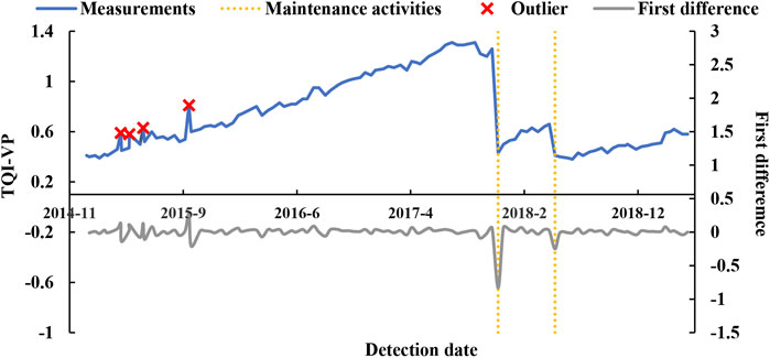
FIGURE 1. The different characteristics of maintenance activities and contaminated measurement data.
Candidate Breakpoints Identified by Adaptive Thresholding Method
The maintenance-points and outliers in the deterioration process are collectively referred to as “candidate breakpoints”. Distinguishing the maintenance-points from outliers within candidate breakpoints will greatly reduce computation load. Accordingly, we develop a method for identifying candidate breakpoints in the deterioration process based on the aforementioned characteristics of maintenance-points and outliers. Constant thresholding is not feasible since track irregularity recovers at different degrees after maintenance among track sections. What is more, outliers cannot be within a predetermined range. Adaptive thresholding provides a solution to this problem (Breier and Branišová, 2015; Wang, 2015). On the basis of adaptive thresholding, we develop a method combining the autoregressive model (referred to as AR) to identify candidate breakpoints in the deterioration process.
Candidate breakpoints are localized by applying this method to the first order difference
Step one: calculate the first order difference
Step two: denote the sliding window as
Step three: fit
Step four: according to the Pauta criterion (
where
Step five: if
The candidate breakpoints identified by the aforementioned method are denoted by
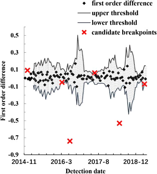
FIGURE 2. A typical realization of the adaptive thresholding method.
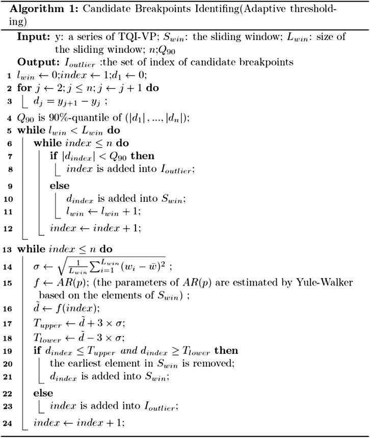
FIGURE 3. Pseudo code for the adaptive thresholding method.
Dynamic Programming for Finding Optimal Fitting Model
Dynamic programming is a multi-stage optimization method and is applicable to various practical problems (Bellman and Dreyfus, 1962). We now consider a method based on the principle of dynamic programming to find an optimal fitting model that achieves the minimum of Eq. 10. Suppose that
For
Considering the tamping will not be operated for a rail track section twice in a month, we set the constraint that
To sum up, the recurrence formulas are
From the previous, it is concluded that
Searching the optimal results under the assumption that there are
The Optimal Value of the Weight Coefficient
The value of the weight coefficient
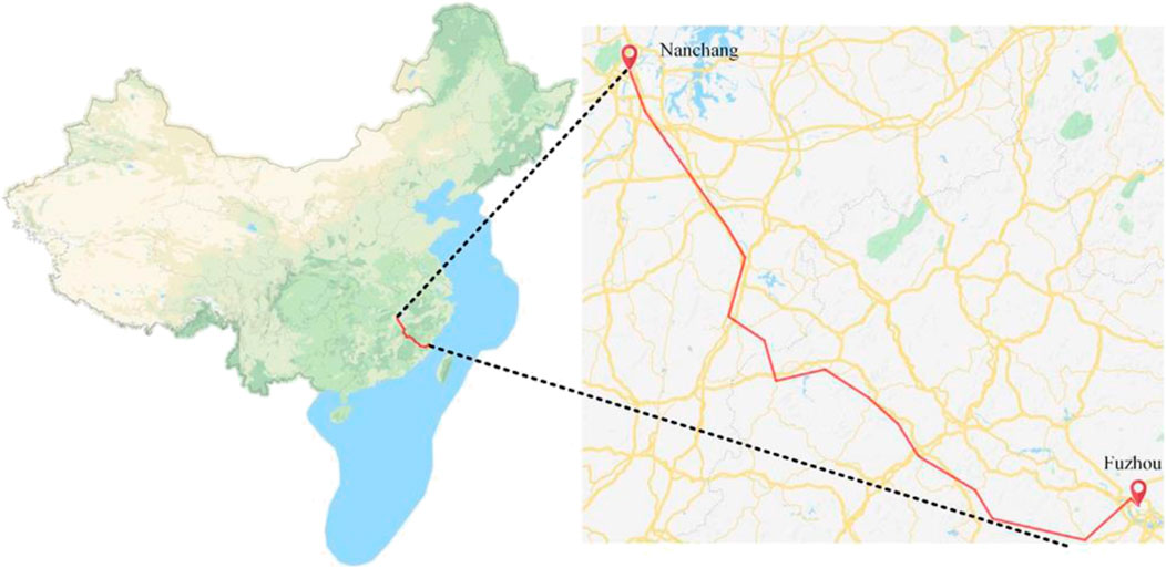
FIGURE 4. Location of the Nanchang-Fuzhou rail line.
To assess the performance of the proposed framework with different values of
where
To find the optimal value of
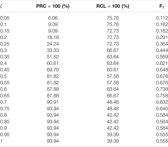
TABLE 1. The statistic results for different values of weight coefficient.
Empirical Analysis
In this section, 33 track sections of 200 m in length are further analyzed to demonstrate the performance of the presented framework with
Performance Analysis
PRC and RCL for each track section are calculated based on the comparison between the estimated maintenance-points and the actual ones. To evaluate the accuracy of the presented framework with the interference of contaminated measurement data, we have investigated the outliers due to the contaminated measurement data of each track section.
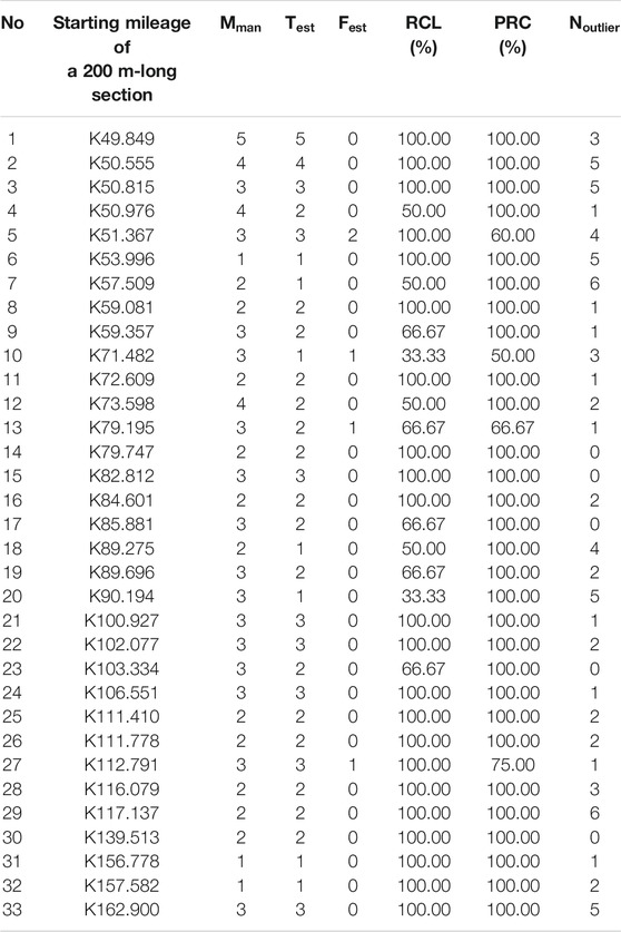
TABLE 2. The evaluation for the identification results of different rail track sections.
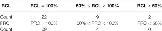
TABLE 3. The distributions of PRC and RCL.
From Table 3, we obtain that the proposed framework owns a high PRC and RCL for most rail track sections. It indicates that this framework is capable of overcoming the disturbance of contaminated measurement data and accurately distinguishing the maintenance-points from outliers within candidate breakpoints. Meanwhile, the RCL of a few sections are not satisfactory. Through analyzing further, we find that it has resulted from the fact that not all maintenance-points are included in the set of candidate breakpoints.
Sensitivity Analysis
A large range of thresholds in Candidate Breakpoints Identified by the Adaptive Thresholding Method Section leads to an excessive number of candidate breakpoints, requiring more time to obtain the minimum of Eq. 10. However, the actual maintenance-points might be left out if the range of thresholds is too small. Accordingly, the sensitivity of this framework to the range of thresholds is discussed in this section. According to Eqs 11, 12, we find that the range of thresholds is significantly affected by the times of
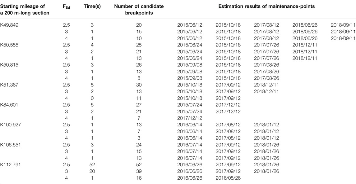
TABLE 4. The comparison results among different values of
From Table 4, we obtain that compared with
Section One: K117 + 137–K117 + 337
This section is on a tangent track. The candidate breakpoints identified by the adaptive thresholding method are shown in Figure 5A. The value of
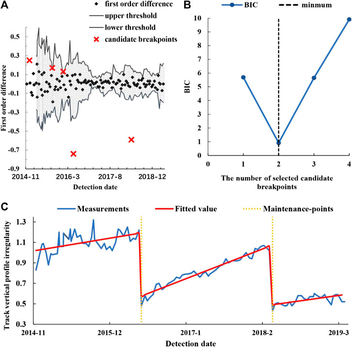
FIGURE 5. The identified maintenance-points and piecewise fitting model of section one: (A) the candidate breakpoints identified by the adaptive thresholding method; (B) the value of BIC for a different number of selected candidate breakpoints; (C) the piecewise fitting model.
Section Two: K162 + 900–K163 + 100
This section is on a curved track. The candidate breakpoints identified by the adaptive thresholding method are shown in Figure 6A, and the value of
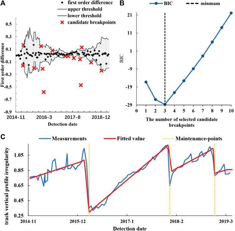
FIGURE 6. The identified maintenance-points and piecewise fitting model of section two: (A) the candidate breakpoints identified by adaptive thresholding method; (B) the value of BIC for a different number of selected candidate breakpoints; (C) the piecewise fitting model.
Conclusion
In this paper, a rail track deterioration modeling framework driven by historical measurement data from CIT is proposed. The modeling framework requires no historical maintenance records and does not assume the quality of track measurement data. The proposed framework formulates the identification of maintenance activities with a model selection optimization problem, based on a modified Bayesian Information Criterion by incorporating an optimized weight for the model complexity component into the objective function. An efficient solution algorithm utilizing adaptive thresholding and dynamic programming is proposed for the model selection problem, taking the characteristics of the effect of maintenance on track deterioration trend.
The proposed track deterioration modeling framework is applied to the historical measurement data from 2014 to 2019 for the nearly 200 km-long track sections of the Nanchang-Fuzhou rail line. Based on that application, the optimal value of the weight coefficient which is incorporated for the model complexity is discussed in The Optimal Value of the Weight Coefficient Section. Moreover, the assessment indicators are calculated based on 33 200 m-long track sections. As the assessment indicators indicate, the proposed framework is capable of accurately identifying the maintenance-points and creating an adaptive piecewise model of the deterioration process.
However, for a few track sections, the estimated maintenance-points are less than the actual ones, which resulted from the fact that not all maintenance-points were included in the set of candidate breakpoints. Therefore, one of the emphases for the next step will be on improving the algorithm to ensure that the set of candidate breakpoints contains all of the maintenance-points.
Data Availability Statement
The raw data supporting the conclusions of this article will be made available by the authors, without undue reservation
Author Contributions
YY: model-establishment and paper-writing. PX, GY, and JL: theoretical-guidance, paper-review and editing. LC: data preprocessing. All authors contributed to the article and approved the submitted version
Funding
This research is supported by the Science and Technology Research and Development Program of China Railway’s “Intelligent Operation and Maintenance Technology for Beijing-Zhangjiakou HSR (Grand No. P2018G051)” project.
Conflict of Interest
GY was employed by China State Railway Group Co., Ltd.
The remaining authors declare that the research was conducted in the absence of any commercial or financial relationships that could be construed as a potential conflict of interest.
References
Bellman, R. E., and Dreyfus, S. E. (1962). Applied dynamic programming. J. Am. Stat. Assoc. 59, 366. doi:10.2307/2282884
Breier, J., and Branišová, J. (2015). A dynamic rule creation based anomaly detection method for identifying security breaches in log records. Wireless Pers. Commun. 94, 1–15. doi:10.1007/s11277-015-3128-1
Brockwell, P. J., Davis, R. A., Berger, J. O., Fienberg, S. E., and Singer, B. (1987). Time series: theory and methods. Berlin, Germany: Springer-Verlag.
Chen, S. S., and Gopalakrishnan, P. S. (1998). “Clustering via the Bayesian information criterion with applications in speech recognition,” in IEEE international Conference on acoustics, speech and signal processing, Seattle, WA, May 15–15, 1998 (IEEE).
Dias, A. (2004). Change-point Analysis for dependence structures in finance and insurance. Risk Measures for the 21st Century. 321–335. Available at SSRN: https://ssrn.com/abstract=2464242
Gang, S., and Ghosh, J. K. (2011). Developing a new BIC for detecting change-points. J. Stat. Plann. Inference 141, 1436–1447. doi:10.1016/j.jspi.2010.10.017
Hall, A. R., Osborn, D. R., and Sakkas, N. (2013). Inference on structural breaks using information criteria. The Manchester School 81, 54–81. doi:10.1111/manc.12017
Hall, A. R., Osborn, D. R., and Sakkas, N. (2015). Structural break inference using information criteria in models estimated by two‐stage least squares. J. Time Ser. Anal. 36, 741–762. doi:10.1111/jtsa.12107
Hannart, A., and Naveau, P. (2012). An improved bayesian information criterion for multiple change-point models. Technometrics 54, 256–268. doi:10.1080/00401706.2012.694780
Jandhyala, V., Fotopoulos, S., Macneill, I., and Liu, P. (2013). Inference for single and multiple change-points in time series. J. Time Ser. Anal. 34 (4), 423–446. doi:10.1111/jtsa.12035
Kotti, M., Benetos, E., Kotropoulos, C., Gustavo, L., and Martins, P. M. (2006). Speaker Change Detection using BIC: a comparison on two datasets. Int. Symp. Commun. Available at at: http://hdl.handle.net/10044/1/12249
Lee, J. S., Hwang, S. H., Choi, Y., and Kim, I. K. (2018). Prediction of track deterioration using maintenance data and machine learning schemes. J. Transport. Eng. 144, 04018045. doi:10.1061/jtepbs.0000173
Li, L., Wen, Z., and Wang, Z. (2016). Outlier detection and correction during the process of groundwater lever monitoring base on Pauta criterion with self-learning and smooth processing,” in Asian simulation conference SCS autumn simulation multi-conference. October 8–11, 2016.
Liu, Y. U., Lei, Y. U., Yi, Q. I., Wang, J., and Wen, H. (2008). Traffic incident detection algorithm for urban expressways based on probe vehicle data. J. Transp. Syst. Eng. Inf. Technol. 8, 36–41. doi:10.1016/s1570-6672(09)60001-5
Lu, Q., Lund, R., and Lee, T. C. M. (2010). AN MDL approach to the climate segmentation problem. Ann. Appl. Stat. 4, 299–319. doi:10.1214/09-aoas289
Meier-Hirmer, C., Senee, A., Riboulet, G., Sourget, F., and Roussignol, M. (2006). “A decision support system for track maintenance,” in Computers in railways X: computer system design and operation in the railway and other transit systems. Editors J. Allan, C. A. Brebbia, A. F. Rumsey, G. Sciutto, S. Sone, and C. J. Goodman (Southampton: Computational Mechanics Publication Ltd), 217.
Mercier, S., Meier-Hirmer, C., and Roussignol, M. (2012). Bivariate Gamma wear processes for track geometry modelling, with application to intervention scheduling. Struct. Infrastruct Eng. 8, 357–366. doi:10.1080/15732479.2011.563090
Perreault, L., Parent, É., Bernier, J., Bobée, B., and Slivitzky, M. (2000). Retrospective multivariate Bayesian change-point analysis: a simultaneous single change in the mean of several hydrological sequences. Stoch. Environ. Res. Risk Assess. 14, 0243–0261. doi:10.1007/s004770000051
Quiroga, L. M., and Schnieder, E. (2010). A heuristic approach to railway track maintenance scheduling. COMPRAIL 2010 114. doi:10.2495/cr100631
Reeves, J., Chen, J., Wang, X. L., Lund, R., and Lu, Q. Q. (2007). A review and comparison of changepoint detection techniques for climate data. J. Appl. Meteorol. Climatol. 46, 900. doi:10.1175/jam2493.1
Schwarz, G. (1978). Estimating the dimension of a model. Ann. Stat. 6, 461–464. doi:10.1214/aos/1176344136
Vale, C., and Lurdes, S. M. (2013). Stochastic model for the geometrical rail track degradation process in the Portuguese railway Northern Line. Reliab. Eng. Syst. Saf. 116, 91–98. doi:10.1016/j.ress.2013.02.010
Veit, P., and Marschnig, S. (2010). “Sustainability IN track - a precondition for high speed traffic,” in ASEM 2010 joint rail conference AMER SOC MECHANICAL ENGINEERS, Urbana, Illinois, April 27–29, 2010, 349–355.
Wang, H. (2015). Anomaly detection of network traffic based on prediction and self-adaptive threshold. Int. J Future Gener. Commun. Networking 8, 205–214. doi:10.14257/ijfgcn.2015.8.6.20
Wang, Y. W., Ni, Y. Q., and Wang, X. (2020). Real-time defect detection of high-speed train wheels by using Bayesian forecasting and dynamic model. Mech. Syst. Signal Process. 139. doi:10.1016/j.ymssp.2020.106654
Watanabe, S. (2012). A widely applicable bayesian information criterion. J. Mach. Learn. Res. 14, 867–897. doi:10.1002/cem.2494
Xi, R., Hadjipanayis, A. G., Luquette, L. J., Kim, T. M., Lee, E., Zhang, J., et al. (2011). Copy number variation detection in whole-genome sequencing data using the Bayesian information criterion. Proc. Natl. Acad. Sci. U.S.A. 108, E1128–E1136. doi:10.1073/pnas.1110574108 |
Xu, P., Liu, R.-K., Wang, F.-T., and Sun, Q.-X. (2012). A novel description method for track irregularity evolution. Int. J. Comput. Intell. Syst. 4, 1358–1366. doi:10.1080/18756891.2011.9727886
Xu, P., Sun, Q., Liu, R., Souleyrette, R. R., and Wang, F. (2015). Optimizing the alignment of inspection data from track geometry cars. Comput. Aided Civ. Infrastruct. Eng. 30, 19–35. doi:10.1111/mice.12067
Xu, P., Sun, Q., Liu, R., and Wang, F. (2011). A short-range prediction model for track quality index. Proc. Inst. Mech. Eng.—F J. Rail Rapid Transit 225, 277–285. doi:10.1177/2041301710392477
Yang, S., Kalpakis, K., and Biem, A. (2014). Detecting road traffic events by coupling multiple timeseries with a nonparametric bayesian method. IEEE Trans. Intell. Transp. Syst. 15, 1936–1946. doi:10.1109/tits.2014.2305334
Yao, Y.-C. (1988). Estimating the number of change-points via Schwarz’ criterion. Stat. Probab. Lett. 6, 181–189. doi:10.1016/0167-7152(88)90118-6
Zhang, N. R., and Siegmund, D. O. (2007). A modified Bayes information criterion with applications to the analysis of comparative genomic hybridization data. Biometrics 63, 22–32. doi:10.1111/j.1541-0420.2006.00662.x |
Keywords: maintenance activities identification, Bayesian information criterion, track irregularity, adaptive thresholding, dynamic programming
Citation: Yang Y, Xu P, Yang G, Chen L and Li J (2021) BIC-Based Data-Driven Rail Track Deterioration Adaptive Piecewise Modeling Framework. Front. Mater. 8:620484. doi: 10.3389/fmats.2021.620484
Received: 23 October 2020; Accepted: 05 January 2021;
Published: 26 February 2021.
Edited by:
Hui Yao, Beijing University of Technology, ChinaReviewed by:
Teng Wang, University of Kentucky, United StatesHualiang Tang, University of Nevada, United States
Copyright © 2021 Yang, Xu, Yang, Chen and Li. This is an open-access article distributed under the terms of the Creative Commons Attribution License (CC BY). The use, distribution or reproduction in other forums is permitted, provided the original author(s) and the copyright owner(s) are credited and that the original publication in this journal is cited, in accordance with accepted academic practice. No use, distribution or reproduction is permitted which does not comply with these terms.
*Correspondence: Peng Xu, cGVuZy54dUBianR1LmVkdS5jbg==