Development of an Elongated Ellipsoid Heat Source Model to Reduce Computation Time for Directed Energy Deposition Process

Introduction

Directed Energy Deposition (DED) is an additive manufacturing process in which focused thermal energy is used to fuse materials by melting as they are being deposited. “Focused thermal energy” means that an energy source (e.g., laser LDED) is focused to melt the material being deposited (Milewski, 2017). As compared to powder bed techniques, material addition rate is much higher in LDED process [up-to 300 cm³/h (Herzog et al., 2016)], hence leading to the possibility of fabricating large parts. Unfortunately, because of the process physics, involving numerous heating and cooling cycles, it leads to generation of unwanted distortion and residual stresses. Researchers have employed Finite Element Method (FEM) to study the thermal gradient induced deformation and stress (Nickel et al., 2001; Zhang et al., 2004; Alimardani et al., 2007; Mukherjee et al., 2017).

FEM techniques to model LDED process is inspired by prior research done on multi-pass weld modeling (Brickstad and Josefson, 1998; Lindgren et al., 1999; Deng and Murakawa, 2006; Bézi and Szávai, 2014; Bonnaud and Gunnars, 2015), because welding process, that has been studied in depth is quite similar to LDED process (Lindgren, 2001a; Lindgren, 2001b; Lindgren, 2001c). In the last few years, modeling techniques from multi-pass welding is applied to Additive Manufacturing (AM) process (Lundbäck and Lindgren, 2011), (Lindgren et al., 2016). But there is a strong difference between welding, LDED and other AM processes, notably in terms of quantity of filler material i.e., deposited material. In welding, filler material volume is relatively low to substrate that requires fewer processing times and computation times. In contrast, in LDED process filler material is much larger in quantity relative to substrate, hence leading to higher processing times. This in turn, requires large computation times (days or months) especially when the same modeling techniques are applied from welding to LDED process. This sort of computation time is not feasible or practical. Because of the large quantity of deposition material in LDED, researchers have focused on different numerical modeling techniques to accurately represent the material addition that leads to reduction in the computation time as well.

Conventionally, researchers have used different numerical techniques to model the material addition for LDED process. A lot of researchers have used the “quiet/active” method that is easy to implement and does not require equation re-numbering but can be computationally expensive (Wang et al., 2008; Chew et al., 2015; Denlinger et al., 2015; Yang et al., 2016; Biegler et al., 2018a; Johnson et al., 2018; Ren et al., 2019). Some researchers have employed “Element Birth” technique that is difficult to implement as it requires solver initialization and equation re-numbering at every simulation, time step elements are activated, but can be computationally faster (Labudovic et al., 2003; Farahmand and Kovacevic, 2014; Biegler et al., 2018b). “Hybrid Activation” method that takes the advantage of both methods of Quiet Activation and Element Birth has been used as well (Heigel et al., 2015; Denlinger and Michaleris, 2016; Biegler et al., 2020). A detailed explanation of all these metal deposition models is well presented in the work (Michaleris, 2014). Another approach that is used by researchers to represent material addition consists of using dynamic mesh based on Arbitrary Lagrangian Eulerian Method (ALE) (Morville et al., 2012; Peyre and Dal, 2017; Morville, 2021).

Besides the material addition modeling, heat source model also influences the computation time. An Elongated Ellipsoid Heat Source Model is developed and demonstrated to reduce the computation time for Selective Laser Melting (SLM) process (Irwin and Michaleris, 2016). The proposed model significantly reduces the problem of temporal discretization originated due to moving heat source and leads to lesser computation time (Irwin and Michaleris, 2016). Also, a dimensionless number is presented that is used to define and optimise the size of computation increment (time-step) that in turn measures and activates the length of the linear segment over which elongated ellipsoid is spread. It was proved that with an increase in size of computation increment, computation time is reduced but it leads to stretch of Elongated Ellipsoid heat Source over longer deposition lengths that results in an increase of computation errors (Irwin and Michaleris, 2016). The model was demonstrated and validated for Ti-6Al-4V and Inconel 625.

Till date, to the best of the knowledge of the author, elongated ellipsoid heat source is not tested and validated for LDED process for any material. Because SLM and LDED processes are different in every aspect related to the physical phenomena and scale, they have therefore different computation requirements due to the size of the laser spot (Heat Source) and build dimensions.

Despite all the contributions and valuable results of the developed models in the past, there is still a need to reduce the computation time for the Numerical Model dedicated to LDED process as the modeling strategy suggested in the literature will lead to impractical computation time. Since, LDED is a material addition process that involves material deposition of track size in hundreds of meters for large part, material deposition model can therefore be an important feature to reduce the computation time of the Numerical Model for LDED process.

This work serves to validate a strategy by introducing efficient material activation by utilising Elongated Ellipsoid Heat Source model in order to reduce the computation time of FEM for LDED process. First, a transient thermal model using quiet activation strategy that employs Double Ellipsoid Heat Source Model (DE) is validated against in situ temperature measurements recorded during the deposition of 20-layer high, Stainless Steel 316L wall builds with varying inter-layer dwell times and laser powers. Next, a transient thermal model with proposed efficient material activation method employing Elongated Ellipsoid Heat Source Model (EE) is used to model the thermal behaviour that leads to drastic decrease of computation time. The computational accuracy and time are then compared with experiment results and Double Ellipsoid Model. A correction factor is introduced to compensate for computation error that increase due to the increase of size of simulation time increment or sub-track segment. At last, an analytical co-relation is developed between simulation time increment/sub-track size, computation accuracy and computation time that is helpful in finding the optimised value of simulation time increments that results in achieving the objective of computation error of less than 10%.

Modeling Approach

The methodology in the proposed numerical model focus on the thermal fields, simplifies the melt-pool fluid and powder dynamics to reduce computational cost. The developed LDED model discretizes the continuous physical process of laser metal deposition into a combination of simulation steps, in which laser travel is considered sequential step-by-step. During each time step, the thermal analysis is performed and the resulting temperature field is saved. The proposed numerical model architecture can be applied to simulate any multi-bead or multi-layer parts.

Thermal Analysis

Assuming a Lagrangian frame Ω and a material point located by r (r ∈ Ω) as the reference, given thermal energy balance at time t, the governing equation can be formulated as follows:

$\rho \left(T\right)C_P\left(T\right)\frac{\partial T\left(r,t\right)}{\partial t}= -\nabla \cdot q\left(r,t\right)+Q\left(r,t\right), r\in \mathit{\Omega }(1)$

where ρ is the material density, C_p is the specific heat capacity, T is the temperature, t is the time, Q is the heat source, and q is the heat conduction flux vector, calculated as:

$\mathit{q}=-k\left(T\right)\nabla T\left(\mathbf{r},t\right)(2)$

Where k is the thermal conductivity of the material.

Table 1 presents the temperature dependent thermal properties for SS 316L (Mills and Mills, 2002). Linear interpolation is used to calculate the properties at any temperature.

TABLE 1

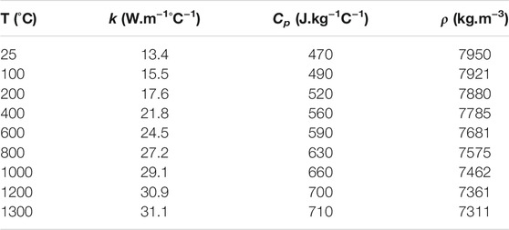
TABLE 1. Temperature dependent material properties of SS 316L (Mills and Mills, 2002).

Heat Source Models

The Single Ellipsoid (SE) heat input model (Goldak) can be used to describe an equivalent to the laser heat source (Goldak et al., 1984) as:

$Q_{\mathit{SE}}= \frac{6\sqrt{3}\mathit{AP}}{\mathit{abc}\pi \sqrt{\pi }}\text{exp}\left(-\frac{3{\left(x+v_{s}t\right)}^2}{a^2} -\frac{3y^2}{b^2} -\frac{3z^2}{c^2}\right)(3)$

The laser power is P and the laser absorption efficiency is A. The value for laser power P is based on measurement, as will be discussed in Experiment Set-Up Section. The value of A is calibrated using the method of reverse calibration by iteratively fitting the simulated temperature field at thermocouple location to match the experiment results described in Ref. (Denlinger et al., 2015). x, y and z are the local coordinates with the origin centred at the ellipsoid where the heat source reaches the maximum intensity and with a moving velocity $v_s$. Parameters a, b and c represent the respective length of the longitudinal, transverse and through the depth semi-axes of the ellipsoid parallel to the local x, y and z axes. Generally, a is taken as the melt-pool length, b is taken as the half width of the deposition bead and c to the melt pool depth (Denlinger et al., 2015).

It has been shown previously that, using single ellipsoid heat source predicts a lower temperature gradient at the front and a higher temperature gradient at the trailing edge as compared to the experiments (Goldak et al., 1984). Therefore, it has been a common practise among the researchers to employ double ellipsoid heat source to be more computationally accurate. The double ellipsoid (DE) Heat Input model (Goldak) is used in the present work to describe the laser heat source (Goldak et al., 1984):

$Q_{\mathit{DE}}= \frac{6\sqrt{3}AP{f}_{f,r}}{a_{f,r}\mathit{bc}\pi \sqrt{\pi }}\text{exp}\left(-\frac{3{\left(x+v_{s}t\right)}^2}{a_{f,r}^2} -\frac{3y^2}{b^2} -\frac{3z^2}{c^2}\right)(4)$

f is a weighting fraction, that determines the energy partition among the front and rear ellipsoid. Typically, different values are employed in the front and rear of the heat source for the longitudinal axis length a (Goldak et al., 1984). The orientation of the double ellipsoid (DE) heat source and coordinate system are depicted in Figure 1A. For the single ellipsoid (SE) heat source the lengths of two ellipsoids are equal (a_f = a_r), hence depicting a single ellipsoid.

FIGURE 1

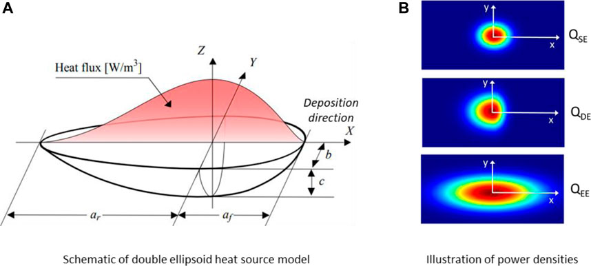
FIGURE 1. (A) Double ellipsoid (DE) heat source model comprised of two ellipsoids, if a_f = a_r it functions as single ellipsoid (SE), (B) Comparison of moving Single Ellipsoid (top) with Double Ellipsoid (centre) and Elongated Ellipsoid (bottom) heat source power.

To accurately model the motion or movement of laser (input heat source), the simulation time increments should be small enough in such a way that the numerical heat source should move less than or equal to half of laser spot size i.e., spot size radius in one-time step (Irwin and Michaleris, 2016). Therefore, in the present work for all cases using Double Ellipsoid Heat Source, computation time-step does not exceed $R/v_s$, where R is laser spot size radius and $v_s$ is laser source/travel speed. In LDED, track length is big and with the specified computation time increment, it can lead to high computation time. Therefore, to reduce the computation time, an elongated ellipsoid line heat input model can be used that averages the single ellipsoid heat source over its path (Irwin and Michaleris, 2016).

$Q_{\mathit{AVERAGE}}= \frac{1}{\Delta t}{\displaystyle {\int }_{t_0}^{t_0+ \Delta t}{Q}_{\mathit{SE}}dt}(5)$

where $t_0$ is the time at beginning of the increment and $\Delta t$ is the duration of time increment over which SE model is averaged. But this averaging over its path will result in large thermal gradients at the edges of each segment especially when the linear segment is large $\left(v_s\Delta t\gg a\right)$ (Irwin and Michaleris, 2016). Therefore, to smooth out the discontinuities at the segment edges, elongated ellipsoid model is developed where peak value of the heat input is at the middle of the sub-track or segment. Power density of elongated ellipsoid at the beginning and end of each segment is half of its peak value that results in smooth distribution over successive linear segments. Thus, Elongated Ellipsoid (EE) line heat input model is also used in present work to describe the laser heat source (Irwin and Michaleris, 2016):

$Q_{\mathit{EE}}= \frac{6\sqrt{3}\mathit{AP}}{\widehat{a}\mathit{bc}\pi \sqrt{\pi }}\text{exp}\left(-\frac{3{\left(x+ v_s\left(t + \frac{1}{2}\Delta t \right)\right)}^2}{{\widehat{a}}^2} -\frac{3y^2}{b^2} -\frac{3z^2}{c^2}\right)(6)$

where the length of each elongated ellipsoid sub-track or segment $\widehat{a}$ is (Irwin and Michaleris, 2016):

$\widehat{a}= \frac{v_s\Delta t}{2}\sqrt{\frac{3}{\mathit{log}2}}(7)$

The main difference between Eq. 3 and Eq. 6 are the introduction of elongated length $\widehat{a}$ in place of a, that stretches the heat distribution in the local x direction and additional (1/2)$\Delta t$ which shifts the peak heat input from the end to the middle of the linear segment or sub-track (Irwin and Michaleris, 2016). Also, the double ellipsoid heat source moves continuously along the path replicating laser movement in experiments with computation time step less than $R/v_s$, the elongated ellipsoid heat source also moves continuously along the path, but enables bigger time steps equal to $\Delta t$ that results in reduction of computation time. A comparison of the energy distribution with three different heat source models SE, DE and EE is shown in Figure 1B. A detailed analysis of the Elongated Ellipsoid Heat Source and its functioning is the presented in the reference work (Irwin and Michaleris, 2016).

Elongated Ellipsoid heat source model allows the simulation of an entire heat source scan in one time increment instead of hundreds of time increment when using Double Ellipsoid or Single Ellipsoid Heat Source. However, taking large time increments also leads to increase in errors as well (Irwin and Michaleris, 2016). Therefore, the track scan is divided into several linear segments (sub-tracks), for each of which, heat source is applied in one simulation time increment.

Thermal Boundary Conditions

The thermal governing equations are supplemented by the initial condition and different types of boundary conditions:

$T\left(\mathit{r},0\right)= T_0\left(\mathit{r},0\right)\mathit{r}\in \mathit{\Omega }(8)$

Thermal radiation $q_{rad}$ is accounted for using the Stefan–Boltzmann law:

$q_{\mathit{rad}}= \epsilon \sigma \left(T^4-T_{\mathit{amb}}^4\right)(9)$

where ε is the surface emissivity, $\sigma$ is the Stefan–Boltzmann constant, T the surface temperature of the workpiece, and $T_{amb}$ is the ambient temperature.

Newton’s law of cooling describes the heat loss due to convection $q_{conv}$:

$q_{\mathit{conv}}=h \left(T-T_{\mathit{amb}}\right)(10)$

where h is the convective heat transfer coefficient.

Latent Heat of Fusion and Marangoni Flow

The effect of latent heat of fusion during the melting and solidification process is accounted by modifying the specific heat capacity $C_p^{\text{*}}$ as in Eq. 1, where $L_f$ (J/kg) is latent heat of fusion, and $T_m$ is melting temperature (Yan et al., 2017).

$C_p^{\text{*}}\left(T\right)=\frac{L_f}{T_m-T_{\mathit{amb}}}+C_p\left(T\right)(11)$

In order to take the convective redistribution of heat in the melt pool due to the fluid flows into account, a higher value of thermal conductivity is considered, hence avoiding integrating complex analytic form in the model (Lampa et al., 1997). Thus, enhanced thermal conductivity factor k^* is assumed in Eq. 2 (Ren et al., 2019):

$k^{\ast }\left(T\right)=\{\begin{array}{c}k\left(T\right),T<T_m\\ 2.5\times k\left(T\right),T\ge T_m\end{array}(12)$

Experiment Set-Up

The modeling approach laid out in Modeling Approach Section is applied to simulate the experimental results acquired for SS 316 L wall builds done with different sets of experiment in an attempt to capture the thermal behaviour. A detailed explanation of the experiment is provided here. Single wall structures were fabricated on a 100 mm long, 50 mm wide, and 3 mm thick SS 316 L substrate (matching material) using a laser-directed energy deposition process. In-house developed MAGIC machine is used for DED system equipped with a 2 kW Diode laser by IPG laser system. Laser and powder are co-focussed at the substrate with laser having a top-hat intensity distribution and incoming powder having Gaussian distribution at the co-focussed point.

For all experiment cases, the depositions are performed at a scan speed of 1 m/min with zig-zag deposition strategy and a powder deposition rate of 13 g/min Stainless Steel 316 L powder feedstock (Oerlikon, grain size 45-106 µm). The laser beam spot size was measured to be 2.2 mm in diameter at the part surface. Figure 2A shows the schematic of substrate and planned wall build and Figure 2B shows DED system with nozzle Figure 2C, co-axial infra-red camera Figure 2D and fixture clamps and Figure 2E shows the wall build for case 1. Each wall build is 20 layers high, 1 bead wide, with a longitudinal zig-zag deposition strategy. For the first set of experiments, effect of waiting time between successive layers (dwell time) is studied by fixing laser power 800 W and changing the dwell time after the deposition of each layer. Dwell times of 0, 5, 10 and 30 s were used for each layer to expose the parts to different cooling time. In the second set of experiments, effect of laser power is studied by keeping a dwell time of 10 s and varying the laser power to 800, 1000, 1200 and 1400 W. Laser scan speed is set to 1 m/min in both tests. Table 2 summarizes the sets of experiments and cases.

FIGURE 2

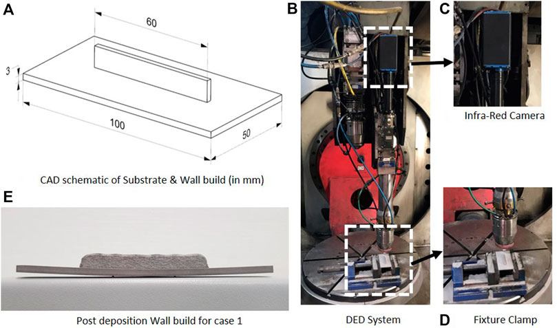
FIGURE 2. (A) Illustrations of CAD, (B) DED system with co-axial nozzle, (C) Co-axially installed infra-red camera, (D) Fixture clamp, (E) Post deposition wall build for case.

TABLE 2

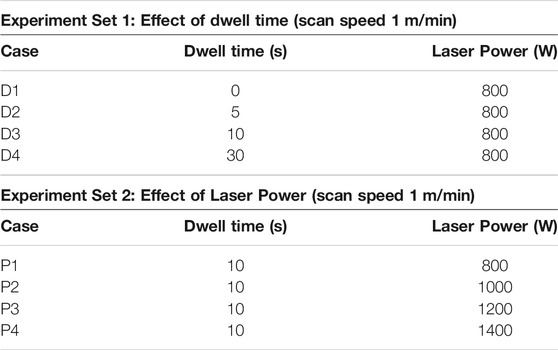
TABLE 2. Description of the cases and process parameters used in the present work.

Temperature Measurement

In situ temperature is measured at two different locations on the bottom face of substrate, as shown in Figure 3A, using Ω GG-K-30 type K thermocouples of 250 µm diameter. The thermocouples have a measurement uncertainty of ± 0.75%. TC 1 and TC 2 are located on the bottom surface of the substrate along the deposition path. The thermocouple signals are read by National Instruments modules 9213. The module record data in Signal Express at a sampling rate of 200 Hz.

FIGURE 3

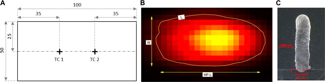
FIGURE 3. (A) Thermocouple locations at bottom face of substrate, (B) Image analysis for In-situ melt-pool length (MP_L) and width (W) recorded by infra-red imaging camera, (C) Post-process melt-pool dilution measured by microscopic analysis.

Melt-Pool Measurement

An Infra-Red imaging camera (NIT system) is used analyse the melt-pool stability and to estimate the melt-pool dimensions based on image analysis. Image acquisition was done at a sampling rate of 200 fps. Image analysis is performed with the Igor Pro software on these images and an average value of melt-pool width (W) and length (MP_L) is measured for each experiment case based on a specific contour level (L), as shown in Figure 3B. The laser penetration depth was also measured for each case by sectioning as recommended in (Goldak et al., 1984) and illustrated in the macrograph shown in Figure 3C. The melt-pool dimensions values given in the Table 3 are then used to calibrate the values of heat source as discussed in previous section.

TABLE 3

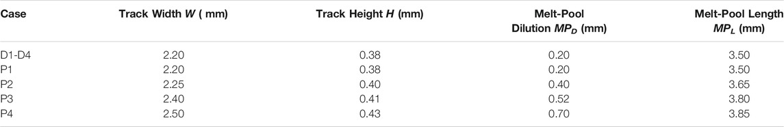
TABLE 3. Wall geometries and Melt-Pool Dimensions.

Numerical Implementation

FEA Solver

The FEM analysis is performed using COMSOL Multiphysics based solver (PARDISO) with the implicit Backward Differentiation Formula (BDF) time stepping method. Adaptive time stepping method is employed rather than strict formulation with maximum time step of $R/v_s$ for DE and $\Delta t$ for EE heat sources. The solver is further adapted specifically to model additive manufacturing technologies in the present work. All simulation cases are performed on an Intel Xeon W-2275, 16 cores, with 128 GB RAM workstation.

FEM Mesh

Figure 4 displays the three-dimensional finite element mesh, generated in COMSOL Multiphysics, used for the thermal model. The same mesh is used for all cases and for different Heat Source models used in the present work. The mesh contains 33,852 Hex-8 elements and 49,790 nodes. Hex-8 elements were chosen because it has been proved that they give more accurate results as compared to tetrahedral elements for the plastic deformation (Benzley et al., 1995), therefore to have same mesh for thermal and mechanical analysis in future work, Hex-8 elements were used. The elements for the deposited material are allotted as 3 per laser spot size and 2 per deposition thickness, making the elements 0.75 × 0.75 × 0.19 mm in volume for experiment case D1, but varies for different experiment cases as track geometry changes. The mesh is coarsened at the substrate as it moves away from the wall builds. A mesh convergence study was done using three different mesh strategies to confirm the accuracy of thermal analysis.

FIGURE 4

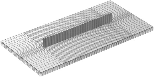
FIGURE 4. Finite Element Mesh of substrate and wall builds.

Material Deposition Modeling

The “quiet” element activation method is used to simulate the deposition of material during the DED process. The elements that represent the wall builds are pre-existing at the beginning of the analysis as shown in Figure 4. But their material properties are rescaled in such a way that it does not affect the computational analysis. In the present work, the thermal conductivity k and specific heat C_p are set to very low values to minimize the heat transfer from active to quiet elements, as follows:

$k_{\mathit{quiet}}= {\alpha }_{k}k(13)$

$C_{P_{\mathit{quiet}}}= {\alpha }_{C_P}{C}_P(14)$

where $k_{\text{quiet}}$ and $C_{P_{\text{quiet}}}$ are the respective thermal conductivity and specific heat for the quiet elements; ${\alpha }_k$ and ${\alpha }_{C_P}$ are the appropriate scaling factors that are usually assigned very small values, for instance, 10^–4 is employed in the present work. The properties of an element are switched from “quiet” to “active” when any Gauss point of the element is consumed by the heat source volume (Eq. 15).

$\exp \left(-\frac{3{\left(x+v_{s}t\right)}^2}{a_{f,r}{ }^2} -\frac{3y^2}{b^2} -\frac{3z^2}{c^2}\right) \ge 5\%(15)$

This means that if the evaluated heat source value at any Gauss point is greater than 5% of the peak intensity, the element will be activated by switching material from quiet to active.

For the elongated ellipsoid line heat input model, material activation is done in the same way of heat source intensity as explained above, but in this case only the activation domain is larger over the deposition path. If the evaluated heat source value at any Gauss point is greater than 50% of the peak intensity, the element turned to active state. The activation criteria of 50% in the deposition direction is explained in the further sections.

$\text{exp}\left(-\frac{3{\left(x+ v_s\left(t_0 + \frac{1}{2}\Delta t \right)\right)}^2}{{\widehat{a}}^2} \right) \ge 50\%(16)$

Model Calibration and Boundary Conditions

To simplify the model, deposited wall build is considered to be a flat rectangular shape with constant layer height and width. This is contrary to the experiments as layer height changes in the few first layers and then reaches a uniform layer thickness. As discussed previously, to develop an accurate thermal model, certain input parameters have to be calibrated against experiment results. The laser absorption efficiency $\left(A\right)$ is taken as 0.4 with reverse calibration of fitting simulated temperature field to experiment results at thermocouple location iteratively as suggested in (Michaleris, 2014). Also, for all experiment cases, as laser spot size is 2.2 mm, laser spot size radius is taken as 1.1 mm. The double ellipsoid heat source dimensions parameters are dependent on experiment cases but follow the same rule i.e., front ellipsoid length $a_f= W/2 and a_r=2a_f, b= W/2 and c=H+M{P}_D$, that represent the double ellipsoid dimensions to be almost equal to experiment melt-pool dimensions for each experiment case. Emissivity $\left(\epsilon \right)$ is temperature dependent, but mean value of 0.6 is taken as widely reported in the literature (Biegler et al., 2018b). The convective heat transfer $\left(h\right)$ coefficient is temperature dependent, but a mean value is taken at the substrate $h=5$ (W.m⁻².K⁻¹) and to consider the effect of forced convection due to the powder carrying argon gas at the wall builds, average convective heat transfer coefficient of $h=25$(W.m⁻².K⁻¹) is taken as widely reported in the literature that it can be in the range of $h=20-60$(W.m⁻².K⁻¹) (Heigel et al., 2015). At the clamped surfaces, the substrate is in contact with metallic fixtures clamps shown in Figure 1 (d). In the numerical model, to reduce the computation time, fixtures clamp is not included, therefore for these surfaces, a higher heat loss is modelled through conductive to convective equivalent heat loss expression similar to Newton’s law of cooling Eq. 10. The thermal conductance at the contact surfaces is thus $h=150$ (W.m⁻².K⁻¹) to model the conductive heat transfer from substrate to the metallic fixture clamps as suggested in (Lu et al., 2019).

Modeling Results and Discussion

Model with Double Ellipsoid Heat Source

The Quiet/Active material activation is well implemented in the model as can be seen in Figure 5. Indeed, during the deposition of the 12th layer, quiet elements of the layer and elements above are not activated and hence does not contribute to the heat transfer, as the material properties of quiet elements are assigned to a dummy material. The current deposition elements and previously deposited layer elements are correctly activated from quiet to active once the activation criteria are satisfied that depends upon the laser travel (Eq. 15). The input heat source absorptivity and heat losses parameters are kept same for all experiment cases as discussed in previous section Model Calibration. Double Ellipsoid heat source dimensions are dependent on experiment cases and is taken following the rule explained in the previous section Model Calibration. The thermal response of the workpiece is calculated by the Double Ellipsoid model and compared to the experimental measurements.

FIGURE 5

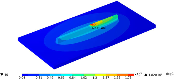
FIGURE 5. Temperature distribution during deposition of 12th layer utilising Quiet/Active material activation.

Figure 6 shows the comparison between experimental results, as measured by thermocouples 1 and 2, and the numerical results at the corresponding nodes in FEM analysis for experiment set 1 (effect of dwell time). As explained in the previous section, due to the experiment set-up, because thermocouple 1 and 2 are at different locations on the substrate but along the deposition line, they record almost same thermal histories with a time offset. Therefore, only Thermocouple 1 results are presented. The thermal response can be classified in 4 different zones depending upon the thermal history. In zone 1, peak temperature for successive build layers increases as layers are building up, in zone 2, peak temperature for successive layers stabilises and there is no further increase of temperature, and in zone 3, peak temperature for successive build layers starts to decrease due to the fact that heat source is moving vertically away from the thermocouple locations and fabricated material starts to increase that also conducts heat leading to the less heat transfer or temperature gradient. In zone 4, once the process is finished, temperature rapidly reduces with respect to time.

FIGURE 6

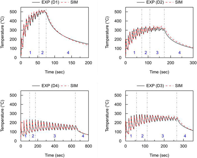
FIGURE 6. Experiments v/s Simulation using Double Ellipsoid (DE) heat source for experiment cases D1-D4 (Effect of dwell time).

In the experiment set 1, analysis of effect of dwell time is studied, as shown in Figure 6. Peak temperature starts to decrease as dwell time increases from 0 to 30 s. Longer dwell times results in lower peak temperatures of 230°C with the 30 s dwell time (D4), while with 0 s dwell time (D1) exceeding 500°C. Therefore, dwell time has a strong influence on temperature evolution as well as the peak temperatures obtained during the deposition process.

For experiment set 1, analysis of effect of dwell time, it is observed that thermal response is changing drastically, not just in terms of peak temperatures, but also in terms of thermal evolution. Table 4 that counts the number of peaks (or layers) observed in the different zones (Z1 to Z4), the number of layers under Zone 1 are decreasing with an increase of dwell time, depicting peak temperature is stabilising at much earlier deposition stage (number of layers). But, the number of layers under Zone 2 and 3 are increasing with an increase of dwell time, depicting that stabilised peak temperature are maintained for longer duration of deposition. Numerical model with calibrated parameters captures the temperature evolution trend and peak temperatures correctly with change of dwell time.

TABLE 4

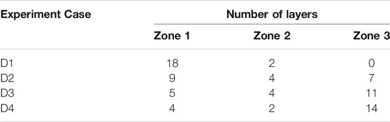
TABLE 4. Classification of layers deposition process according to temperature gradient for experiment cases D1-D4 (Effect of dwell time).

In experiment set 2, analysis of effect of laser power is studied, as shown in Figure 7. Peak temperature keeps on increasing as laser power increases from 800 to 1400 W. higher laser power results in higher peak temperatures of 480°C with 1400 W laser power (P4), and only 280°C with 800 W laser power (P1). Therefore, laser power has a strong influence on peak temperature, but does not influence the trend of temperature evolution obtained during the deposition process.

FIGURE 7

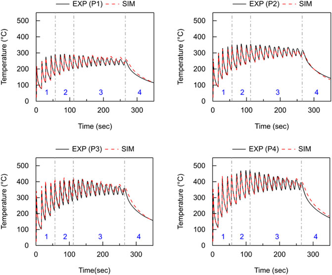
FIGURE 7. Experiments v/s Simulation using Double Ellipsoid (DE) heat source for experiment cases P1-P4 (Effect of laser power).

For experiment set 2 (analysis of effect of laser power), it is observed that thermal response is changing peak temperatures drastically, but does not influences the thermal gradient. As it can be seen in Table 5, number of layers under Zone 1, 2 and 3 remains same depicting that temperature trend is lifted upwards (increase of peak temperature). Higher peak temperatures are recorded because of the increase of laser power, but the thermal gradient remains the same. As can be seen in Table 5, peak temperature is stabilised at fifth layer, stabilises for next 4 layers and then starts to decrease as heat source is moving vertically away from thermocouple locations for all experiment cases (P1-P4).

TABLE 5

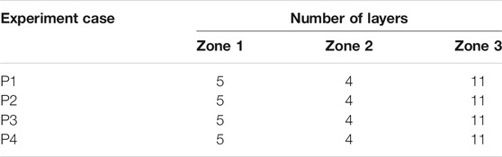
TABLE 5. Classification of layers deposition process according to temperature gradient for experiment cases P1-P4 (Effect of laser power).

The results of the transient thermal analyses are in close agreement with the experimental results as can be seen in Figure 6 and Figure 7. Errors between experiment and simulation results are calculated by comparing instances in time.

$\% \mathit{Error}= \frac{100{{\displaystyle \sum }}_{i=1}^n\left|\frac{{\left(T_{\mathit{exp}}\right)}_i- {\left(T_{\mathit{sim}}\right)}_i}{{\left(T_{\mathit{exp}}\right)}_i}\right|}{n}(17)$

where n is the total number of simulation time increments between the beginning and end of the deposition, i is the current time increment, T_sim is the simulated temperature, and T_exp is the measured temperature. The largest error at thermo-couple is found to be 3.91%.

Table 6 shows the computation time and percent error at both thermocouples TC1 and TC2 for all cases. For experiment set 1 (D1 to D4), it can be clearly seen that with the increase of dwell time, that leads to increase in number of time increments leading to increase in computation time. For experiment set 2 (P1 to P4), it can be observed that with an increase in laser power, that leads to an increase in simulation peak temperature at the melt-pool region i.e., higher thermal gradient, that leads to slight increase of computation time.

TABLE 6

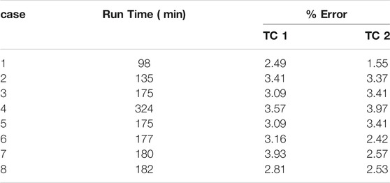
TABLE 6. Cases examined for Thermal Model Validation (Double Ellipsoid).

Model with Elongated Ellipsoid Heat Source

To reduce the computation time, elongated ellipsoid model is used to reduce the number of simulation time steps by dividing the complete track in number of linear sub-tracks, with each sub-track is solved in one simulation time step. Different track size (sub-track) is chosen for material activation presented in Table 7 and a comparison is done with the experiment results to make a compromise between computation speed and accuracy.

$K_E= \frac{v_s\Delta t}{a}(18)$

TABLE 7

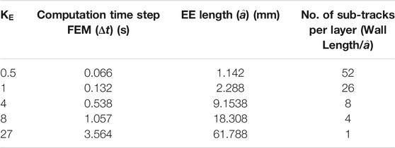
TABLE 7. Elongated Ellipsoid (EE) heat source parameters used in the present work.

As shown in Figure 8A, 5 different simulation time increments are chosen, where K_E = 0.5 represents heat source movement of R with a time step of $R/v_s$, hence the ellipsoid is not elongated and that is same as in the case of double ellipsoid heat source, K_E = 4 represents heat source averaging over a segment of 8R with a simulation time step of $8R/v_s$ and K_E = 27 represents heat source averaging over a segment of 54R with a simulation time step of $54R/v_s$, that is averaging over the complete track, activating the complete track and performing heat transfer analysis in 1 simulation time increment.

FIGURE 8

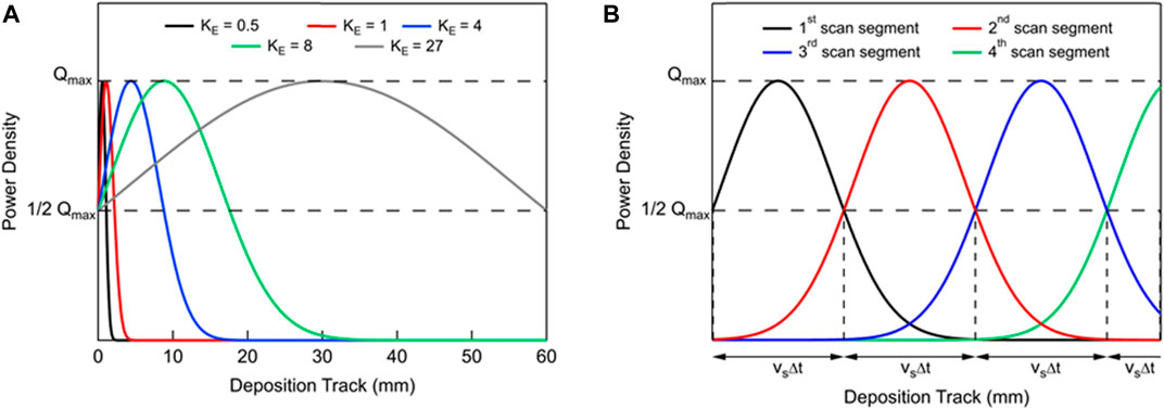
FIGURE 8. (A)Illustration of K_E (sub-track sizes) at first computation time step of Elongated Ellipsoid (EE) heat Source, (B) Power Intensity for subsequent sub-tracks of elongated ellipsoid (EE) with K_E = 8 over the deposition track.

The movement of the elongated ellipsoid heat source is such that there is a smooth distribution of power intensity over the successive scan segments. The power intensity at the start and end of each scan segment is half of its peak value, resulting in a smooth distribution over the successive segments of a track as shown in Figure 8B. And this is the reason why activation criteria for elongated ellipsoid (EE) heat source model is 50% that accounts for the half of its peak value in the deposition direction. Of course, increasing the factor K_E helps in reducing the total computation time, but it also leads to the increase of computation error. Thus, effect of sub-track size activation on temperature evolution at thermocouple location is shown in Figure 9. K_E of 0.5 (∆t = $R/v_s$) gives the same accurate results as we observed with Double Ellipsoid (DE) heat source with a simulation time step of $R/v_s$. As explained in the section further, computation error increase with K_E, while computation time drops, as shown in Figure 10.

FIGURE 9

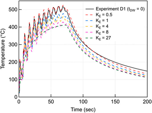
FIGURE 9. Effect of K_E (sub-track sizes) on temperature evolution at Thermocouple location in experiment Case D1.

FIGURE 10

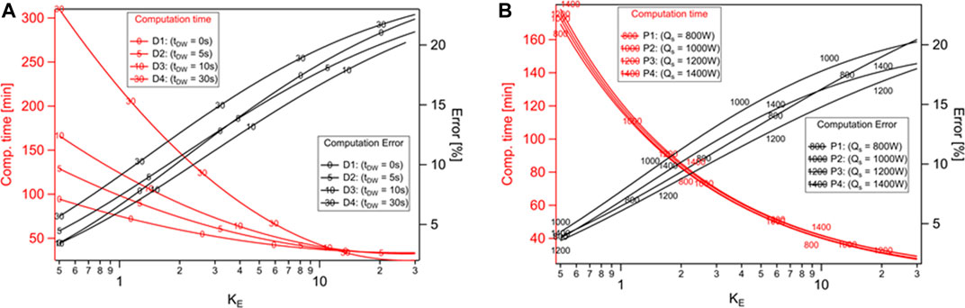
FIGURE 10. Effect of K_E on computation time and accuracy of the numerical model with the elongated ellipsoid heat source (A) D1-D4 (effect of dwell time), (B) P1-P4 (effect of laser power).

For all experiment cases, simulation is performed to find out the effect of K_E on computation time and accuracy. Figure 10A shows the results for D1-D4 (effect of dwell time). For case D1, with increase in K_E from 0.5 to 27, computation time reduces drastically from 90 to 35 min, but leads to an increase of error from 2 to 22%. For case D2, with respect to increase of K_E, computation time reduction is more drastic from 130 to 36 min and computation error increases from 3 to 21%. For case D3 and case D4 as well, computation time reduction is more as dwell time is increasing but computation error is also increasing.

Figure 10B shows the results for all cases P1-P4 (effect of laser power). For case P1-P4, with increase in K_E from 0.5 to 27, computation time reduces from 175 to 25 min, but leads to an increase of error from 2 to 21%. Computation time reduction is exponential (3–4 times reduction) when K_E is increased from 0.5 to 4. But then the trend in computation time becomes linear when K_E is increased from 4 to 27 (not even half). Computation error increases linearly with an increase in K_E. So, an intelligent compromise needs to be done to reduce the computation time but also keeping in mind the computation error as well. In this work, the objective is that computational error should be less than 10%, that is well accepted in the scientific and industrial community. Keeping this in mind, K_E $=4$ seems to satisfy both the objectives of reducing the computation time drastically but also keeping computation error less than 10%. Further increase of K_E results in computation time reduction, but computation error exceeds 20% when K_E = 27. However, with the introduction of elongated ellipsoid (EE) heat source, it is noticed that there is a drop-down of the temperature at melt-pool scale (local scale) as well as part scale (global scale) e.g., thermocouple locations that is far away from the deposition region as shown in Figure 9. This modification of the thermal behaviour (especially, melt-pool scale) will surely impact the local mechanical response of the sample. Therefore, same analysis needs to be performed to verify if the optimised value of K_E found in thermal analysis is also valid for mechanical response e.g., distortion and residual stresses.

Correction Factor

Due to the increase in K_E (sub-track length), computation time reduces exponentially, but it also leads to increase in computation errors. To compensate those errors, a variable source correction factor K_Q is introduced that leads to an increase in source intensity in elongated ellipsoid model, as shown in the equation below.

$Q_{\mathit{EE}}= \frac{6\sqrt{3}{\mathit{APK}}_Q}{\widehat{\mathit{a}}\mathit{bc}\pi \sqrt{\pi }}\exp \left(-\frac{3{\left(x+ v_s\left(t_0 + \frac{1}{2}\Delta t \right)\right)}^2}{{\widehat{a}}^2} -\frac{3y^2}{b^2} -\frac{3z^2}{c^2}\right)(19)$

With the introduction of K_Q, distribution and peak intensity over the ellipsoid is increased artificially. Thus, the correct value of K_Q should be dependent upon the value of K_E, so calibration of source correction factor is done with respect to different sub-track size for all experiment cases. Then for the correct value of correction factor that should be dependent upon the size of sub-track $(K_E$), Calibration of correction factor is done with respect to sub-track size ($K_E$) for all cases. K_E = 0.5 does not elongate the ellipsoid. So, to analyse the effect of correction factor, values of K_E starting from 1 to 27 is used, because K_E = 0.5 using Elongated Ellipsoid does averaging over a sub-track of R, i.e., SE or DE with a simulation time step of $R/v_s$ i.e., conventional simulation increment.

As it can be seen in Figure 11 with K_E values (1, 4, 8 and 27) shown in black vertical lines, for experiment cases D1-D4 (effect of dwell time), with an increase in K_E, computation error increases as we have seen in the previous section, source correction factor K_Q value is also increasing to compensate for this increase in computation error with an increase in K_E. Therefore, there is a direct relation between K_E and K_Q, that is helpful in achieving the second objective to reduce the computation error. With the introduction of K_Q, K_E = 8, 16 can also be utilised as computation error falls below 10% which was not the case previously. As it can be seen in Figure 12, for experiment cases P1-P4 (effect of laser power), same relation is established between K_E and K_Q. In this set of experiments also, K_E = 8, 16 can now be used in heat transfer analysis as computation error falls below 10%. So, with the introduction of K_Q, computation error is reduced along with reduction of computation time as higher values of K_E yields desired accurate results. With the introduction of correction factor, there is no significant impact on the computation time of analysis.

FIGURE 11

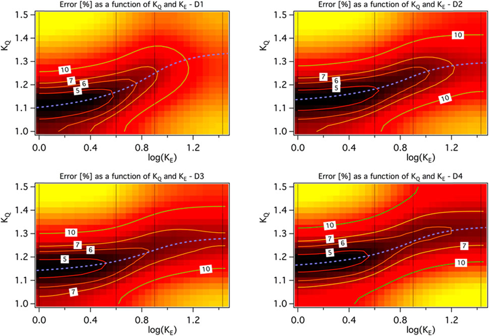
FIGURE 11. Domain of computation accuracy as a function of K_E and K_Q for the experiment cases D1-D4 (effect of dwell time). The minimum error is pointed out with a blue dashed line.

FIGURE 12

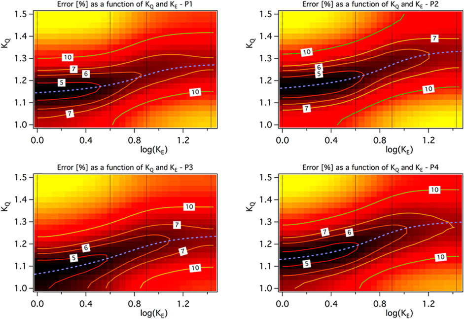
FIGURE 12. Domain of computation accuracy as a function of K_E and K_Q for the experiment cases P1-P4 (effect of laser power). The minimum error is pointed out with a blue dashed line.

As it can be seen in Figure 13, for experiment case D1 with K_E = 4, with the introduction of correction factor K_Q using EE heat source model, temperature evolution at thermocouple location shifts upwardly due to the increase of heat intensity. K_Q values of 1.1 and 1.2 seems to be well compensating the effect of K_E that leads to underprediction of temperature evolution, but with further increase of K_Q values of 1.3, 1.4 and 1.5, it can be seen that it over-compensates the thermal error generated due to K_E, and starts to yield higher computation error. Therefore, a correlation between K_E and K_Q should be established for different process parameters that yields minimum computation error for elongated ellipsoid (EE) heat source.

FIGURE 13

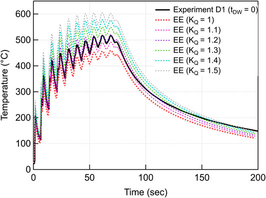
FIGURE 13. Effect of source correction factor (K_Q) on temperature evolution at thermocouple location for K_E = 4 (sub-track size) for experiment case D1.

Correlation

For all experiment cases D1-D4 and P1-P4, it can be seen in Figure 14 that for most experiment cases, with an increase of K_E from 0.5 to 8, there is also an increase in correction factor from K_Q = 1 to 1.25, that leads to minimum computation error for temperature history at thermocouple location. But with further increase of K_E from 8 to 27, further increase in values of K_Q is not required. Therefore, a correlation between K_E and K_Q is recommended in this work that yield to minimum computation error.

FIGURE 14

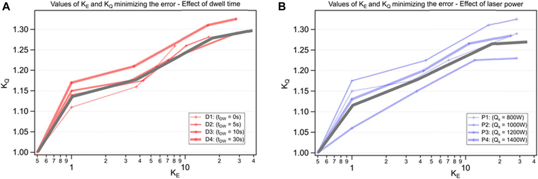
FIGURE 14. Identification of a source correction factor (K_Q) for different sub-tract sizes (K_E), for different experiment cases. Recommended correlation between these parameters is pointed out in grey line.

Conclusion

• DE heat source model with small time increments $(\le R/v_s)$ correctly predicts temperature evolution with an average computation accuracy of more than 96%, but leads to long computation time due to thousands of simulation time increments.

• EE heat source model with different K_E values significantly reduces computation times (up to 10 times) while yielding average computation accuracy of more than 75–95%.

• A source correction factor (K_Q) for Elongated Ellipsoid (EE) heat source model is presented that reduces the average computation error within 5% at thermocouple location.

• A correlation is then found that is helpful in finding the co-relation between simulation time increments, computation time and error. Correlation is shown to be dependent of variables laser power and dwell time.

• Thermal model with DE heat source and EE heat source with different K_E and K_Q works efficiently for different process parameters justifying the versatility of the model.

In the future, correlation can also be extended to other materials and process parameters and can be applied to a thermo-mechanical model to prove the efficiency of the Elongated Ellipsoid heat source model in the prediction of residual stress and deformation as well.

Data Availability Statement

The original contributions presented in the study are included in the article/Supplementary Material, further inquiries can be directed to the corresponding author.

Author Contributions

VN, MC, and TE contributed to the modeling of the study. VN, LS, and DB organized and performed the experiments. VN, LS, and TE did the data treatment and analysis. VN wrote the first draft of the manuscript. VN, MC, TE, and DB contributed to manuscript revision, read, and approved the submitted version.

Funding

This work was supported and funded by French Ministry of Higher Education, Research and Innovation under CIFRE programme (CIFRE no: 2018/1509). This study was also supported by the PAMPROD project that is funded by BPI FRANCE under PSPC program N°2018-PSPC-09.

Conflict of Interest

The authors declare that the research was conducted in the absence of any commercial or financial relationships that could be construed as a potential conflict of interest.

Publisher’s Note

All claims expressed in this article are solely those of the authors and do not necessarily represent those of their affiliated organizations, or those of the publisher, the editors and the reviewers. Any product that may be evaluated in this article, or claim that may be made by its manufacturer, is not guaranteed or endorsed by the publisher.

References

Alimardani, M., Toyserkani, E., and Huissoon, J. P. (2007). 3D Dynamic Numerical Approach for Temperature and thermal Stress Distributions in Multilayer Laser Solid Freeform Fabrication Process. Opt. Lasers Eng. 45, 1115–1130. doi:10.1016/j.optlaseng.2007.06.010

CrossRef Full Text | Google Scholar

Benzley, S. E., Perry, E., Merkley, K., Clark, B., and Sjaardema, G. (1995). “A Comparison of All Hexagonal and All Tetrahedral Finite Element Meshes for Elastic and Elasto-Plastic Analysis,” in Proceedings, 4th International Meshing Roundtable, 179–191.

Google Scholar

Bézi, Z., and Szávai, S. (2014). Repair Weld Simulation of Austenitic Steel Pipe. Adv. Mater. Res. 1029, 194–199. doi:10.4028/www.scientific.net/amr.1029.194

CrossRef Full Text | Google Scholar

Biegler, M., Elsner, B. A. M., Graf, B., and Rethmeier, M. (2020). Geometric Distortion-Compensation via Transient Numerical Simulation for Directed Energy Deposition Additive manufacturingGeometric Distortion-Compensation via Transient Numerical Simulation for Directed Energy Deposition Additive Manufacturing. Sci. Technology Welding Joining 25, 468–475. doi:10.1080/13621718.2020.1743927

CrossRef Full Text | Google Scholar

Biegler, M., Graf, B., and Rethmeier, M. (2018). In-situ Distortions in LMD Additive Manufacturing walls Can Be Measured with Digital Image Correlation and Predicted Using Numerical Simulations. Addit. Manuf. 20, 101–110. doi:10.1016/j.addma.2017.12.007

CrossRef Full Text | Google Scholar

Biegler, M., Marko, A., Graf, B., and Rethmeier, M. (2018). Finite Element Analysis of In-Situ Distortion and Bulging for an Arbitrarily Curved Additive Manufacturing Directed Energy Deposition Geometry. Addit. Manuf. 24, 264–272. doi:10.1016/j.addma.2018.10.006

CrossRef Full Text | Google Scholar

Bonnaud, E., and Gunnars, J. (2015). Three Dimensional Weld Residual Stresses Simulations of Start/Stop and Weld Repair Effects. Proced. Eng. 130, 531–543. doi:10.1016/j.proeng.2015.12.260

CrossRef Full Text | Google Scholar

Brickstad, B., and Josefson, B. L. (1998). A Parametric Study of Residual Stresses in Multi-Pass Butt-Welded Stainless Steel Pipes. Int. J. Press. Vessels Piping 75, 11–25. doi:10.1016/S0308-0161(97)00117-8

CrossRef Full Text | Google Scholar

Chew, Y., Pang, J. H. L., Bi, G., and Song, B. (2015). Thermo-mechanical Model for Simulating Laser Cladding Induced Residual Stresses with Single and Multiple Clad Beads. J. Mater. Process. Technology 224, 89–101. doi:10.1016/j.jmatprotec.2015.04.031

CrossRef Full Text | Google Scholar

Deng, D., and Murakawa, H. (2006). Numerical Simulation of Temperature Field and Residual Stress in Multi-Pass Welds in Stainless Steel Pipe and Comparison with Experimental Measurements. Comput. Mater. Sci.Computational Mater. Sci. 37, 269–277. doi:10.1016/j.commatsci.2005.07.007

CrossRef Full Text | Google Scholar

Denlinger, E. R., Heigel, J. C., and Michaleris, P. (2015). Residual Stress and Distortion Modeling of Electron Beam Direct Manufacturing Ti-6Al-4V. Proc. Inst. Mech. Eng. B: J. Eng. Manufacture 229, 1803–1813. doi:10.1177/0954405414539494

CrossRef Full Text | Google Scholar

Denlinger, E. R., and Michaleris, P. (2016). Effect of Stress Relaxation on Distortion in Additive Manufacturing Process Modeling. Addit. Manuf 12, 51–59. doi:10.1016/j.addma.2016.06.011

CrossRef Full Text | Google Scholar

Farahmand, P., and Kovacevic, R. (2014). An Experimental–Numerical Investigation of Heat Distribution and Stress Field in Single- and Multi-Track Laser Cladding by a High-Power Direct Diode Laser. Opt. Laser Technology 63, 154–168. doi:10.1016/j.optlastec.2014.04.016

CrossRef Full Text | Google Scholar

Goldak, J., Chakravarti, A., and Bibby, M. (1984). A New Finite Element Model for Welding Heat Sources. Metall. Trans. Bmtb 15, 299–305. doi:10.1007/BF02667333

CrossRef Full Text | Google Scholar

Heigel, J. C., Michaleris, P., and Reutzel, E. W. (2015). Thermo-mechanical Model Development and Validation of Directed Energy Deposition Additive Manufacturing of Ti–6Al–4V. Addit. Manuf. 5, 9–19. doi:10.1016/j.addma.2014.10.003

CrossRef Full Text | Google Scholar

Herzog, D., Seyda, V., Wycisk, E., and Emmelmann, C. (2016). Additive Manufacturing of Metals. Acta Mater. 117, 371–392. doi:10.1016/j.actamat.2016.07.019

CrossRef Full Text | Google Scholar

Irwin, J., and Michaleris, P. (2016). A Line Heat Input Model for Additive Manufacturing. J. Manuf. Sci. Eng. 138 (no. 11). doi:10.1115/1.4033662

CrossRef Full Text | Google Scholar

Johnson, K. L., Rodgers, T. M., Underwood, O. D., Madison, J. D., Ford, K. R., Whetten, S. R., et al. (2018). Simulation and Experimental Comparison of the Thermo-Mechanical History and 3D Microstructure Evolution of 304L Stainless Steel Tubes Manufactured Using LENS. Comput. Mech.Comput Mech. 61, 559–574. doi:10.1007/s00466-017-1516-y

CrossRef Full Text | Google Scholar

Mills, K. C., ‘Fe - 316 Stainless Steel’, in Recommended Values of Thermophysical Properties for Selected Commercial Alloys, K. C. Mills, Ed. Cambridge, England: Woodhead Publishing, 2002, Fe - 316 Stainless Steel, pp. 135–142. doi:10.1533/9781845690144.135

CrossRef Full Text | Google Scholar

Labudovic, M., Hu, D., and Kovacevic, R. (2003). A Three Dimensional Model for Direct Laser Metal Powder Deposition and Rapid Prototyping. J. Mater. Sci. 3838, 35–49. doi:10.1023/a:1021153513925

CrossRef Full Text | Google Scholar

Lampa, C., Kaplan, A. F. H., Powell, J., and Magnusson, C. (1997). An Analytical Thermodynamic Model of Laser Welding. J. Phys. D: Appl. Phys. 30, 1293–1299. doi:10.1088/0022-3727/30/9/004

CrossRef Full Text | Google Scholar

Lindgren, L.-E. (2001). Finite Element Modeling and Simulation of Welding Part 1: Increased Complexity. J. Therm. Stresses 24, 141–192. doi:10.1080/01495730150500442

CrossRef Full Text | Google Scholar

Lindgren, L.-E. (2001). Finite Element Modeling and Simulation of Welding. Part 2: Improved Material Modeling. J. Therm. Stresses 24, 195–231. doi:10.1080/014957301300006380

CrossRef Full Text | Google Scholar

Lindgren, L.-E. (2001). Finite Element Modeling and Simulation of Welding. Part 3: Efficiency and Integration. J. Therm. Stresses 24, 305–334. doi:10.1080/01495730151078117

CrossRef Full Text | Google Scholar

Lindgren, L.-E., Lundbäck, A., Fisk, M., Pederson, R., and Andersson, J. (2016). Simulation of Additive Manufacturing Using Coupled Constitutive and Microstructure Models. Addit. Manuf. 12, 144–158. doi:10.1016/j.addma.2016.05.005

CrossRef Full Text | Google Scholar

Lindgren, L., Runnemalm, H., and Näsström, M. (1999). Simulation of Multipass Welding of a Thick Plate. Wiley. doi:10.1002/(SICI)1097-0207(19990330)44:9<1301:AID-NME479>3.0.CO;2-K

CrossRef Full Text | Google Scholar

Lu, X., Lin, X., Chiumenti, M., Cervera, M., Hu, Y., Ji, X., et al. (2019). Residual Stress and Distortion of Rectangular and S-Shaped Ti-6Al-4V Parts by Directed Energy Deposition: Modelling and Experimental Calibration. Additive Manufacturing 26, 166–179. doi:10.1016/j.addma.2019.02.001

CrossRef Full Text | Google Scholar

Lundbäck, A., and Lindgren, L.-E. (2011). Modelling of Metal Deposition. Finite Elem. Anal. Des. 47, 1169–1177. doi:10.1016/j.finel.2011.05.005

CrossRef Full Text | Google Scholar

Michaleris, P. (2014). Modeling Metal Deposition in Heat Transfer Analyses of Additive Manufacturing Processes. Finite Elem. Anal. Des. 86, 51–60. doi:10.1016/j.finel.2014.04.003

CrossRef Full Text | Google Scholar

Milewski, J. (2017). Additive Manufacturing of Metals. From Fundam. Technology Rocket Nozzles, Med. Implants Custom Jewelry 258. doi:10.1007/978-3-319-58205-4

CrossRef Full Text | Google Scholar

Morville, S., Carin, M., Peyre, P., Gharbi, M., Carron, D., Le Masson, P., et al. (2012). 2D Longitudinal Modeling of Heat Transfer and Fluid Flow during Multilayered Direct Laser Metal Deposition Process. J. Laser Appl. 24, 032008. doi:10.2351/1.4726445

CrossRef Full Text | Google Scholar

Mukherjee, T., Zhang, W., and DebRoy, T. (2017). An Improved Prediction of Residual Stresses and Distortion in Additive Manufacturing. Comput. Mater. Sci. 126, 360–372. doi:10.1016/j.commatsci.2016.10.003

CrossRef Full Text | Google Scholar

Nickel, A. H., Barnett, D. M., and Prinz, F. B. (2001). Thermal Stresses and Deposition Patterns in Layered Manufacturing. Mater. Sci. Eng. A. 317, 59–64. doi:10.1016/S0921-5093(01)01179-0

CrossRef Full Text | Google Scholar

Peyre, P., and Dal, M., Sebastien POUZET, and O. Castelnau, ‘Simplified Numerical Model for the Laser Metal Deposition Additive Manufacturing Process’, J. Laser Appl., vol. 29, no. 2, p. Article number 022304, 2017, doi:10.2351/1.4983251

CrossRef Full Text | Google Scholar

Ren, K., Chew, Y., Fuh, J. Y. H., Zhang, Y. F., and Bi, G. J. (2019). Thermo-mechanical Analyses for Optimized Path Planning in Laser Aided Additive Manufacturing Processes. Mater. Des. 162, 80–93. doi:10.1016/j.matdes.2018.11.014

CrossRef Full Text | Google Scholar

Morville, S., ‘Modélisation multiphysique du procédé de Fabrication Rapide par Projection Laser en vue d’améliorer l’état de surface final’, phdthesis, Université de Bretagne Sud, 2012. Accessed: 2021. [Online]. Available at: https://tel.archives-ouvertes.fr/tel-00806691.

Google Scholar

Wang, L., Felicelli, S., Gooroochurn, Y., Wang, P. T., and Horstemeyer, M. F. (2008). Optimization of the LENS® Process for Steady Molten Pool Size. Mater. Sci. Eng. A. 474, 148–156. doi:10.1016/j.msea.2007.04.119

CrossRef Full Text | Google Scholar

Yan, L., Li, W., Chen, X., Zhang, Y., Newkirk, J., Liou, F., et al. (2017). Simulation of Cooling Rate Effects on Ti–48Al–2Cr–2Nb Crack Formation in Direct Laser Deposition. JOMJom 69, 586–591. doi:10.1007/s11837-016-2211-8

CrossRef Full Text | Google Scholar

Yang, Q., Zhang, P., Cheng, L., Min, Z., Chyu, M., and To, A. C. (2016). Finite Element Modeling and Validation of Thermomechanical Behavior of Ti-6Al-4V in Directed Energy Deposition Additive Manufacturing. Addit. Manuf. 12, 169–177. doi:10.1016/j.addma.2016.06.012

CrossRef Full Text | Google Scholar

Zhang, L., Reutzel, E. W., and Michaleris, P. (2004). Finite Element Modeling Discretization Requirements for the Laser Forming Process. Finite Element Modeling Discretization Requirements Laser Forming Processint. J. Mech. Sci. 46, 623–637. doi:10.1016/j.ijmecsci.2004.04.001

CrossRef Full Text | Google Scholar