Developing a regional environmental corrosion model for Q235 carbon steel using a data-driven construction method

1 Introduction

Metals are ubiquitous in industries, such as construction and manufacturing, and therefore, their safe and reliable use is crucial for applications (Vazirinasab et al., 2018; Shi and Ming, 2017). The corrosion of metals due to the environment reduces the service life of buildings and equipment. This result in safety concerns and a waste of natural resources (Melchers, 2019; Li et al., 2022). The annual global economic loss caused by corrosion is estimated to be approximately four trillion US dollars (Li et al., 2015). To address this issue, corrosion mechanisms must be understood, and reliable corrosion models must be established, which will allow for better material selection and corrosion protection (Faqih and Zayed, 2021; Deng et al., 2020).

The atmospheric corrosion of metals is influenced by temperature, relative humidity (RH), rainfall, and various pollutants (Cai et al., 2018; Wang et al., 2021). Many corrosion models have been developed based on these environmental factors and can be categorized as black-box and gray-box models. Black-box models are obtained by analyzing the characteristics of the input and output (Varol et al., 2014; Díaz and López, 2007; Wen et al., 2009), while gray-box models are established by statistical analysis based on prior experience (Zhan et al., 2021). Black-box models consider more influential factors and have higher accuracy than gray-box models (Zhi et al., 2021). However, a major disadvantage of black-box models is the complex and inexplicable internal structure of the model. Conversely, gray-box models have strong interpretability, simple structures, and low requirements for modeling expertise (Panchenko et al., 2017).

Since the early 20th century, various types of mathematical models within the gray-box model category have been established to extrapolate changes in atmospheric corrosion rates depending on a variety of environmental factors. The models that were developed between 1968 and 1984 considered less than three environmental factors and used relatively simple functional forms, such as linear and power functions (Klinesmith et al., 2007). The dose-response function (DRF) proposed in the ICP Materials report was the first functional model to predict the corrosion rate of metals depending on atmospheric environmental factors (Tidblad et al., 2001). This model combined power, exponential, and linear functions. The DRF coefficients were modified to integrate the data from the ISO CORRAG and MICAT Programs (Mikhailov et al., 2004), rendering the model widely accepted in the field of metal corrosion research. The International Organization for Standardization incorporated the DRF into the ISO9223-2012 standard to quantify the corrosion loss of carbon steel, zinc, copper, and aluminum after environmental exposure for 1 year.

Although the DRF was considered to have made significant progress in revealing the mechanism of environmental corrosion, several studies have shown major discrepancies between predicted and actual corrosion rates. For example, the DRF was found to be inaccurate in predicting the corrosion rate of weathering steel, zinc, and copper at nine sites in Switzerland considering a variety of environmental types (Leuenberger-minger et al., 2002). The corrosion rates of four ISO9223-2012 standard metal materials were measured at 15 test sites in Iran and compared with the corresponding DRF values. It was found that the DRF was not applicable in most areas of Iran (Shiri and Rezakhani, 2019). Similar results were obtained in a metal corrosion study conducted in Cuba (Castaneda et al., 2018). These discrepancies were primarily due to the two climatic seasons (rainy season and winter season) in Cuba.

The inaccurate prediction of atmospheric corrosion rates using the DRF can be attributed to two main factors. First, most of the data used in the DRF are obtained in Europe and South America (Chico et al., 2017). Since geographical location directly impacts the atmospheric environment (Noyes et al., 2009), the DRF cannot be accurately applied to other areas, particularly those with dissimilar climates. Second, the DRF considers four environmental factors: temperature, RH, sulfur dioxide concentration, and chloride concentration. However, other potential environmental factors that may affect atmospheric corrosion need to be incorporated to improve the generality of the model and to fully describe the complex corrosion phenomenon.

Herein, we developed a regional environmental corrosion model (RECM) to predict atmospheric corrosion based on the measured corrosion rates of carbon steel exposed for 1 year in China. Our model includes nine different environmental factors: temperature, RH, rainfall, SO₂, NO₂, O₃, CO, particulate matter (PM10), and chloride deposition. The method to build the RECM includes four modules: data preprocessing, environmental region division, key factor selection, and regional model generation. The results from this study proved that the RECM of carbon steel has high precision and can adapt to China’s environmental characteristics. The entire model can be implemented automatically using a computer.

2 Materials and methods

2.1 Data sources

Corrosion data were obtained from carbon steel atmospheric corrosion tests conducted by the State Grid Corporation of China over the course of 1 year at 2040 sites in 25 provinces in China. The tests were performed according to the ISO9226-2012 standard. A standard sample of Q235 carbon steel was ground, removed of oil, and exposed to the environment for 1 year. After the one-year-long exposure, all corrosion products were removed, and the corrosion rate (R_corr) of the sample was calculated using the weight loss. Three parallel samples were set at each site to find the average R_corr value.

Environmental data were obtained from 2,162 meteorological monitoring stations at the China National Meteorological Science Data Center and 1,605 air pollutant monitoring stations at the National Urban Air Quality Real-time Publishing Platform of the China General Environmental Monitoring Station. Chloride deposition was measured according to the ISO9225-2012 standard using the dry plate method. The annual average value of each environmental data point was calculated, and Kriging interpolation was used to calculate the values at each test site. All data used in this study are summarized in Table 1.

TABLE 1

TABLE 1. Unit of data.

2.2 Data preprocessing

Corrosion data obtained from long-term exposure tests generally exhibit a high degree of scattering owing to the difficulty of precisely controlling the testing conditions. In certain cases, samples exposed to similar environmental conditions may show large differences in corrosion rates, sometimes the differences even exceed the two corrosion grades defined in ISO9223-2012 standard. Herein, we used a preprocessing step to correct for abnormal data and to improve the quality of the prediction model.

This preprocessing treatment applies a distance threshold to the K-means algorithm (Chiang and Mirkin, 2010), which aggregates the data based on similar environmental conditions and further eliminates abnormal data. The process comprises the following steps.

(1)The parameters must be defined. The number of data groups is represented by $N$. Each data group includes environmental data ($X$) and R_corr ($Y$). The number of cluster centers ($K$) is generally defined as $N/2<K<2N/3$. The distance ($d$) between the two samples $x_1$ and $x_2$ in the sample space is represented by $d\left(x_1,x_2\right)$. The value of the threshold ($Q$) is dependent on the data.

(2) Normalize $X$.

(3) The constraints of the K-means algorithm are as follows:

(a) $C=\left\{C_1,C_2\dots C_k\right\}$ denotes the initial cluster center set. For $C_i,C_j\in C$, $d\left(C_i,C_i\right)>Q$ must be satisfied. If $d\left(C_i,C_i\right)\le Q$, the identity of the cluster center of a sample is removed randomly.

(b) $C_L$ denotes the cluster center of class $L$. For any $C_L$ and sample $n$, if $d\left(C_L,n\right)\ge Q$, $n$ is not classified in class $L$.

(4) As shown in Figure 1, we designed the following rules for eliminating abnormal data according to the corrosion classification of ISO9223-2012 standard:

(a) If there is only one sample in the class, the sample and class are retained.

(b) If there are two samples in the class and the corrosion grade difference between them is more than one grade, both are removed. If the corrosion grade difference is one or less, both samples are retained.

(c) If there are more than two samples in the class, the corrosion grade with the largest number of samples is considered the benchmark. If the difference between a sample in the class and the benchmark is more than one grade, the sample is removed.

FIGURE 1

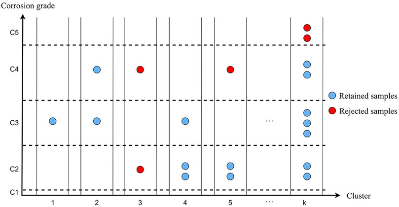
FIGURE 1. Schematic of abnormal data rejection rules.

2.3 Environmental region division

Owing to the complexity of the corrosion environment data, a single model cannot accurately describe the relationship between corrosion behavior and environmental factors without data simplification. The environmental information can be simplified by dividing the environmental regions based on the basic law of corrosion. This allows data in the same region to have a more uniform change law.

Because the regional division is based on environmental indicators, it is directly related to R_corr. Studies indicate that temperature and RH are the main factors affecting the atmospheric corrosion of carbon steel (Cai et al., 2018; Wang et al., 2021; Soares et al., 2009; Cole et al., 2009; Li et al., 2019). To explore their relationship with corrosion, the average R_corr was calculated for each unit of temperature and RH. This relationship and the polynomial fitting of the mean change are shown in Figure 2. Synergistic effects of temperature and RH on R_corr are observed. A significant change in synergy is detected between R_corr and temperature at approximately 10 and 15°C. This is different from the results of a previous study (Tidblad et al., 2002) that showed that a significant change in synergistic effects is only observed at 10°C. The synergy between R_corr and RH changes at approximately 52% and 68% RH. Previously, the threshold of RH was only considered where corrosion occurred (Roberge et al., 2002). Based on these results, we set the boundaries of regional division with respect to the temperature to 9–11°C and 14–16°C and with respect to RH to 50%–54% and 66%–70%.

FIGURE 2

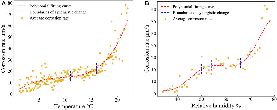
FIGURE 2. Trend curve of mean change of R_corr with respect to (A) temperature and (B) RH.

In addition to temperature and RH, the effect of chloride on atmospheric corrosion is non-trivial (Bojórquez et al., 2021; Liu et al., 2019). Chloride in the atmosphere originates from salt spray generated by the ocean and can spread up to approximately 50 km from the coastline (Cole et al., 2003). Herein, the chloride concentrations in inland regions more than 50 km from the coastline were constant. Therefore, the distance from the coast (D_c) was used as an environmental indicator for regional division.

2.4 Key corrosion factor selection

All the environmental factors listed in Table 1 can affect metal corrosion (Oesch, 1996; Chen et al., 2005; Corvo et al., 2005; Syed, 2008; Rouillard et al., 2009; Li et al., 2013; Nguyen et al., 2013; Nyrkova et al., 2013; Wang et al., 2013; Pei et al., 2020), and coupling relationships exist among these factors (Meng et al., 2021). The role of each environmental factor in the corrosion of carbon steel depends on the region. Therefore, key corrosion factors should be selected for each region.

Previous studies typically used correlation analysis to evaluate the importance of environmental factors. However, the correlation analysis method assumes that all other factors are constant, which is not reflected in real-life corrosion datasets. To address this issue, we used random forest (Breiman, 2001) to assess feature importance and for feature selection in this study. Random forest is based on the combination of decision trees and measures the importance of factors by calculating the model prediction error caused by incorrect input factors. While considering the individual influence of each factor, we also considered the multivariate interaction of other factors (Strobl et al., 2008). The process we used is as follows.

(1) The dataset was divided into training and testing sets. The random forest model was trained using the training data set, and the model accuracy was verified using the testing data set. The root-mean-square error (RMSE, $L$) was used as the evaluation index.

$RMSE=\sqrt{\frac{1}{n}{{\displaystyle \sum }_{i-1}^n\left(y_i-\stackrel{\wedge }{y_i}\right)}^2}$

(2) The set of environmental factors is denoted as $F=\left\{F_1,F_2,\cdots F_I\right\}$. The observation sequence of $F_i\left(i\le I\right)$ in the testing set was randomly shuffled. The sequence of observations excluding $F_i$ remained constant, and the new test set was named $D{F}_i$. This was repeated several times until every environmental factor in $F$ had been perturbed once and a new testing set $D{F}_i\left(i\le I\right)$ was obtained. The prediction accuracy $FL=\left\{F{L}_1,F{L}_2,\cdots F{L}_I\right\}$ of the model on each test set in $D=\left\{D{F}_1,D{F}_2,\cdots D{F}_I\right\}$ was calculated again, where $F{L}_i$ corresponds to the prediction accuracy after the observation sequence of scrambled factor $F_i$.

(3) N-fold cross-validation was performed in step (2). The prediction results for any $F{L}_i$, namely, $F{L}_{ij}(j=\mathrm{1,2}\cdots n$), were obtained. The difference between $L$ and $F{L}_{ij}$ was used to calculate the importance of features. The average value of cross-validation was recorded in the set $IM=\left\{I{M}_1,{IM}_2,\cdots I{M}_I\right\}$, where $I{M}_i$ corresponds to the importance of features of factor $F_i$:

$I{M}_i=\frac{1}{n}\left({\displaystyle \sum }_j^n\left(L_j-F{L}_{ij}\right)\right)$

(4) The above equation was normalized to $IM=\left\{I{M}_1,{IM}_2,\cdots I{M}_I\right\}$, rendering values between 0 and 1. The result is the importance score of each feature.

2.5 Regional model generation

Two main methods can be used for constructing mathematical corrosion models. One is to describe the effects of environmental variables directly by combining linear functions (Van den Steen et al., 2016). The other is to use the non-linear transformation of the environmental variables for modeling. An example of this method is the DRF in the ISO9223-2012 standard.

The performance of a model is generally dependent on the dataset. However, it is impractical to find a universal model that can be applied to all datasets (Ho and Pepyne, 2002). Herein, we adopted a data-driven perspective with the objective of combining as many environmental factors as possible in limited quantities to improve the expression ability of our model. We tested several model structures and chose the following structure based on its performance.

$R_{corr}={\displaystyle \sum }_{i=1}^S{\omega }_i{A}_i+{\omega }_j{\displaystyle \sum }_{j=1}^S\ln \left(A_j\cdot T\cdot P\right)+{\omega }_{2S+1}T+{\omega }_{2S+2}P$

$P=\left\{\begin{array}{l}\ln \left(Rain\right),I{M}_{Rain}\ge I{M}_{RH}\\ RH,I{M}_{Rain}<I{M}_{RH}\end{array}\right.$

Where ${\omega }_1,{\omega }_2,\cdots {\omega }_{2S+2}$ are undetermined parameters; $A_1,A_2,\cdots A_S$ are pollutant variables, and ${IM}_{RH}$ and ${IM}_{Rain}$ correspond to the factor importance of RH and rainfall described in Section 2.4. In regions where rainfall has a higher impact on corrosion than RH, $P$ represents rainfall. Similarly, $P$ represents RH in regions where RH has a higher corrosion impact than rainfall.

This model consists of two parts. The first part, ${\displaystyle \sum }_{i=1}^S{\omega }_i{A}_i+{\omega }_{2S+1}T+{\omega }_{2S+2}P$, is a weighted sum of environmental factors. The second part, ${\omega }_j{\displaystyle \sum }_{j=1}^S\ln \left(A_j\cdot T\cdot P\right)$, is a combination of regulators to improve the non-linear fitting ability of the model. Both parts together describe the overall effect of the environment on the corrosion rate. Multiple linear regression was used to obtain the undetermined parameters of each regional model. The regional models were then combined to form the RECM of carbon steel.

3 Results

In total, 326 groups of abnormal data were removed through data preprocessing. As shown in Figure 3, a decrease in the number of outliers is observed with the data preprocessing. However, the overall distribution of the data remains consistent. The remaining 1714 groups of data were used to construct the RECM.

FIGURE 3

FIGURE 3. Schematic of a small area causing potential modeling issues.

A key consideration during the regional division process is the size of the region. Small regions may contain very few test sites to construct the model and therefore will have a decreased significance in practical engineering applications (Figure 4). The most suitable combinations of regional boundaries obtained by the computer program are 9°C, 16°C, 50% RH, and 69% RH. Figure 5 shows the process of merging regions with small sample sizes into conditionally adjacent regions, while Table 2 presents the regional conditions and number of samples in each region. Figures 6A,B show the maps of the annual average temperature and RH, respectively. These maps were superimposed with Geographical Information System (GIS) technology to generate the regional division (Figure 6C). The key corrosion factors selected by random forest for each region and the mathematical model of each region are listed in Table 3 and Table 4, respectively. In the equations in Table 4, the symbols of air pollutants represent corresponding variables, $T$ is the temperature, $Rain$ is rainfall, and $Cl$ is chloride deposition.

FIGURE 4

FIGURE 4. Process and results of region merging.

FIGURE 5

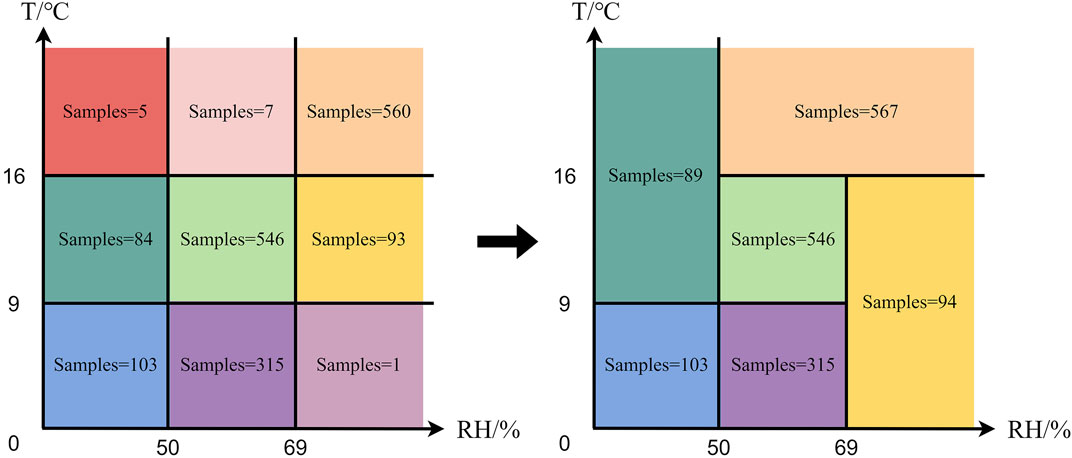
FIGURE 5. Box plots for dataset before and after data preprocessing.

TABLE 2

TABLE 2. Results of environmental region division.

FIGURE 6

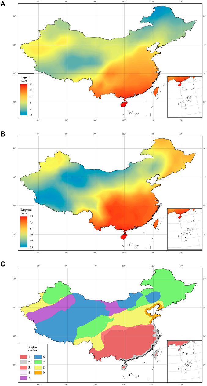
FIGURE 6. Map of annual averages of (A) temperature and (B) RH, and (C) results of region division.

TABLE 3

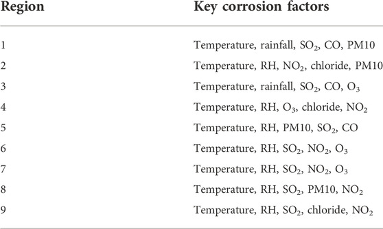
TABLE 3. Key corrosion factors in each region.

TABLE 4

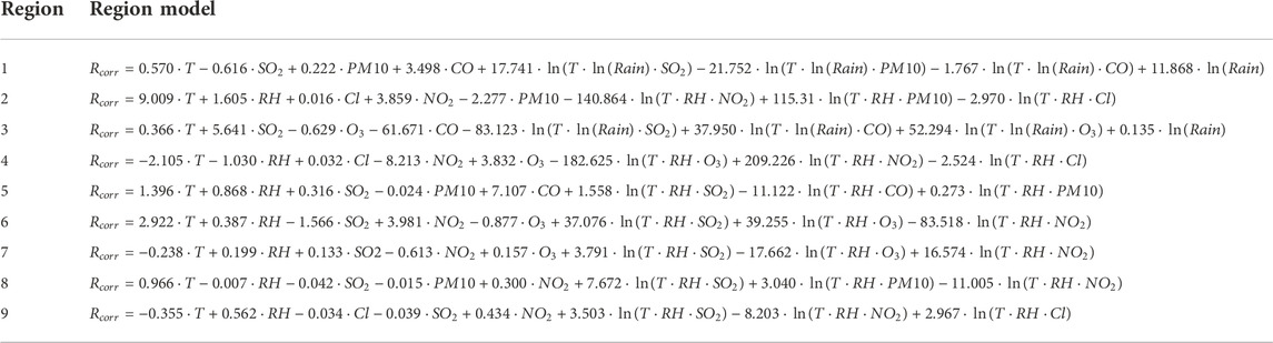
TABLE 4. Model of each region.

The RMSE, mean absolute error (MAE), and classification accuracy (CA) were used to evaluate the performance of each regional model and were calculated as follows.

$MAE=\frac{1}{n}{\displaystyle \sum }_{i=1}^n\left|y_i-\stackrel{\wedge }{y_i}\right|$

$CA=\frac{M}{n}$

In these equations, $y_i$ is the value fitted by the RECM; $\stackrel{\wedge }{y_i}$ is the real value; $M$ is the number of samples with fitted corrosion grades that match the actual corrosion grade, and $n$ is the total number of samples.

Figure 7 shows the fitting results of the RECM for each region. Within each region, the RECM shows good fitting within a specific corrosion rate range, where the sample points have a dense distribution, which leads to good overall performance of the model. However, outside of this specific range, the fitting performance is not satisfactory. As shown Figures 7F,G, the R_corr values measured in these two regions are mostly in the range of 0–20 μm/a and 0–30 μm/a, and the fitting results to the data in this range are excellent. But beyond this range the fitting results become suboptimal. This is mainly due to the limitations of low-order functions in expressing non-linear relations. In addition, the RECM does not distinguish the data near the boundary of corrosion grade ideally, which results in the decline of classification accuracy in some regions (Figures 7A,B). Overall, the RECM outperforms the DRF in accurately predicting corrosion rates in all nine regions (Table 5).

FIGURE 7

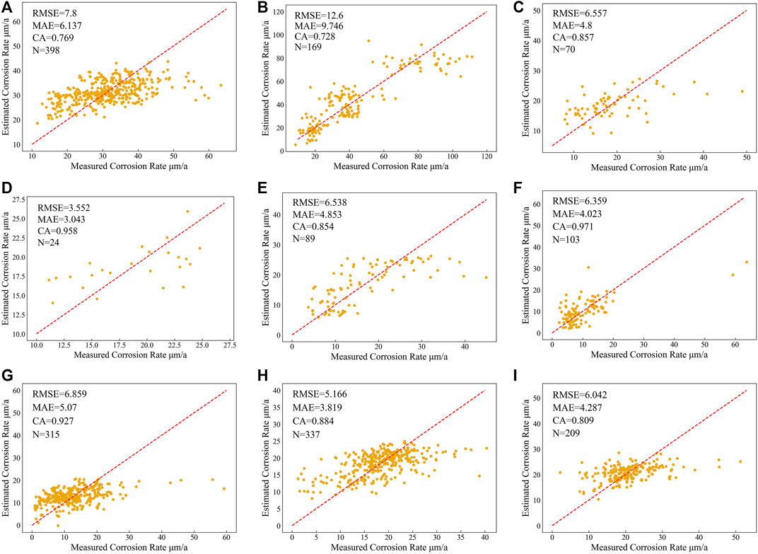
FIGURE 7. Fitting results of RECM on (A) region 1, (B) region 2, (C) region 3, (D) region 4, (E) region 5, (F) region 6, (G) region 7, (H) region 8, and (I) region9.

TABLE 5

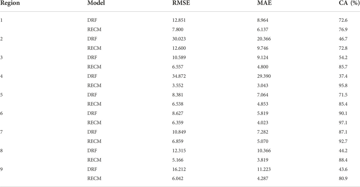
TABLE 5. Performance comparison between RECM and DRF.

4 Discussion

4.1 Differences in key corrosion factors between regions

Table 3 presents the key corrosion factors that specifically impact each region. In every region, temperature has a significant effect on corrosion. Because RH and rainfall are highly correlated, one, but not both, of these factors were assigned to each region. Temperature and RH were considered appropriate factors for determining regional divisions. Notably, regions 1, 2, 3, and 4 are in the same latitude range. Regions 1 and 3 are non-marine sites. Therefore, it was assumed that rainfall has a higher impact on corrosion than RH. We assumed that the metal surfaces are wet at night and during rainfall in the non-marine sites and that the RH remains high for a long time in marine sites (Cole et al., 2009). Chloride was selected as a key corrosion factor in the three marine regions, which verified the effect of the marine salt spray on corrosion.

Additionally, we examined the concentrations of various pollutants in each region and selected those with significant concentrations as key corrosion factors in the corresponding regions. The effect of SO₂ on the atmospheric corrosion of carbon steel is well established. In seven of the considered regions, SO₂ was selected as a key corrosion factor. The concentration of SO₂ in regions 2 and 4 was relatively low and therefore considered to have an insignificant impact on corrosion. Similarly, PM10 was chosen as a critical corrosion factor for regions 5 and 8 owing to its significantly high concentration in those regions. Regions 2, 4, and 8 had higher concentrations of NO₂ as compared to other regions owing to the many adjacent tall buildings and dense traffic flow. NO₂ had a significant effect on corrosion in these regions. The concentration of O₃ in the atmosphere is affected by many factors, such as solar radiation intensity, temperature, and RH. Regions 6 and 7 contain high concentrations of O₃ owing to the plateau terrain areas, rendering it an important corrosion factor in these regions.

Other pollutants can also indirectly influence atmospheric corrosion. For example, CO can react with other air pollutants and lead to corrosion. Notably, CO was included as a key factor in regions 1, 3, and 5. The concentrations of other various pollutants were high in certain regions but were not considered key factors leading to corrosion. As compared to conventional correlation analysis, the method proposed herein can better identify non-linear relationships in the data and the factors that have the highest influence on corrosion.

4.2 Corrosion map

The corrosion of Q235 carbon steel was calculated using the RECM for regions throughout China. These results were paired with visualization technology to develop a corrosion rate map (Figure 8). The R_corr values decrease from low to high latitudes, which is consistent with the trend of temperature variation with latitude. Areas with a higher number of heavy industries in the north, such as the Shanxi Province and Hebei Province, have higher R_corr values. The R_corr values in marine areas are generally higher than those in non-marine areas because of higher atmospheric chloride concentrations. The R_corr values of marine areas near the Bohai Sea, such as the northern part of Shandong Province, eastern part of Tianjin City, and southwestern part of Liaoning Province, are relatively low. This could be because the Bohai Sea is an inland sea with fewer waves, and therefore, lower amounts of chloride are present. In central Inner Mongolia, high elevation variations and large diurnal temperature differences (Hu et al., 2015) lead to frequent dry-wet processes on the metal surface, which may result in high R_corr values in this region. This mathematical model can be adjusted to suit specific geographical locations and used to predict the R_corr values in those regions to adopt targeted corrosion protection measures.

FIGURE 8

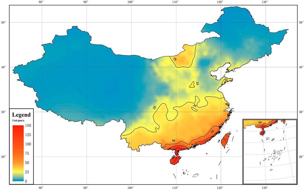
FIGURE 8. Corrosion map of Q235 carbon steel in China.

4.3 Computerization

The method of constructing the RECM is modularized such that the computer program can automatically generate the RECM, as shown Figure 9. This is of considerable significance for corrosion assessment and protection in buildings and production. Significantly, some parameters need to be set according to different materials and data, such as the threshold ($Q$) in data preprocessing and the parameters of random forest in the selection of key factors.

FIGURE 9

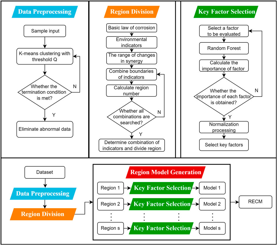
FIGURE 9. Flowchart for constructing RECM.

5 Conclusion

In summary, we developed an RECM for estimating the corrosion of Q235 carbon steel in China. This model is suitable for predicting carbon steel corrosion in China and addresses issues related to existing approaches. The following conclusions can be drawn from this study.

(1) We simplified large datasets and complex information through data preprocessing and environmental region division. Samples with similar environmental conditions were aggregated, which resulted in a close relationship between the corrosion rate and environmental factors.

(2) Considering the coupling effect of various environmental factors in metal atmospheric corrosion, random forest was used to replace the common correlation analysis method. This allowed for an accurate calculation of the degree of influence of various environmental factors on corrosion.

(3) A mathematical regional corrosion model was constructed using key corrosion factors as input variables.

(4) The method for constructing the RECM is modularized and can be automatically implemented by a computer. This implies that the model can be applied in the construction of mathematical models for the environmental corrosion of other materials.

Data availability statement

The datasets presented in this article are not readily available because the dataset involves sensitive information. Requests to access the datasets should be directed to DF, fdm2003@163.com.

Author contributions

YL and DF, methodology, software, formal analysis and original draft preparation. XC and DZ, Conceptualization and editing. The rest of the authors, investigation, data curation and validation. All authors contributed to manuscript revision and read and approved the submitted versions.

Funding

This research was funded by the Science and technology project of State Grid Corporation of China (5200-202058470A-0-0-00) and the Science and Technology Basic Resources Investigation Project (No.2019FY101404).

Conflict of interest

YC is employed by Electric Power Research Institute of State Grid Fujian Electric Power Company Limited. WH, YC, and BY are Employed by State Grid Smart Grid Research Institute Co., Ltd., China.

The remaining authors declare that the research was conducted in the absence of any commercial or financial relationships that could be construed as a potential conflict of interest.

Publisher’s note

All claims expressed in this article are solely those of the authors and do not necessarily represent those of their affiliated organizations, or those of the publisher, the editors and the reviewers. Any product that may be evaluated in this article, or claim that may be made by its manufacturer, is not guaranteed or endorsed by the publisher.

References

Bojórquez, J., Ponce, S., Ruiz, S. E., Bojórquez, E., Reyes-Salazar, A., Barraza, M., et al. (2021). Structural reliability of reinforced concrete buildings under earthquakes and corrosion effects. Eng. Struct. 237, 112161. doi:10.1016/j.engstruct.2021.112161

CrossRef Full Text | Google Scholar

Breiman, L. (2001). Random forests. Mach. Learn. 45 (1), 5–32. doi:10.1023/A:1010933404324

CrossRef Full Text | Google Scholar

Cai, Y., Zhao, Y., Ma, X. B., Zhou, K., and Chen, Y. (2018). Influence of environmental factors on atmospheric corrosion in Dynamic Environment. Corros. Sci. 137, 163–175. doi:10.1016/j.corsci.2018.03.042

CrossRef Full Text | Google Scholar

Castañeda, A., Valdés, C., and Corvo, F. (2018). Atmospheric corrosion study in a harbor located in a tropical island. Mater. Corros. 69 (10), 1462–1477. doi:10.1002/maco.201810161

CrossRef Full Text | Google Scholar

Chen, Z. Y., Zakipour, S., Persson, D., and Leygraf, C. (2005). Combined effects of gaseous pollutants and sodium chloride particles on the atmospheric corrosion of copper. Corrosion 61 (11), 1022–1034. doi:10.5006/1.3280618

CrossRef Full Text | Google Scholar

Chiang, M. M.-T., and Mirkin, B. (2010). Intelligent choice of the number of clusters in K-means clustering: An experimental study with different cluster spreads. J. Classif. 27 (1), 3–40. doi:10.1007/s00357-010-9049-5

CrossRef Full Text | Google Scholar

Chico, B., Fuente, D. D. L., Díaz, I., Simancas, J., and Morcillo, M. (2017). Annual Atmospheric Corrosion of carbon steel worldwide. an integration of ISOCORRAG, ICP/UNECE and MICAT databases. Materials 10 (6), 601. doi:10.3390/ma10060601

PubMed Abstract | CrossRef Full Text | Google Scholar

Cole, I. S., Ganther, W. D., Furman, S. A., Muster, T. H., and Neufeld, A. K. (2009). Pitting of zinc: Observations on atmospheric corrosion in tropical countries. Corros. Sci. 52 (3), 848–858. doi:10.1016/j.corsci.2009.11.002

CrossRef Full Text | Google Scholar

Cole, I. S., Ganther, W. D., Paterson, D. A., King, G. A., Furman, S. A., and Lau, D. (2003). Holistic model for atmospheric corrosion: Part 2 - experimental measurement of deposition of marine salts in a number of long range studies. Corros. Eng. Sci. Technol. 38 (4), 259–266. doi:10.1179/147842203225008886

CrossRef Full Text | Google Scholar

Corvo, F., Minotas, J., Delgado, J., and Arroyave, C. (2005). Changes in atmospheric corrosion rate caused by chloride ions depending on rain regime. Corros. Sci. 47 (4), 883–892. doi:10.1016/j.corsci.2004.06.003

CrossRef Full Text | Google Scholar

Deng, Z. H., Yin, H. Q., Jiang, X., Zhang, C., Zhang, G. F., Xu, B., et al. (2020). Machine-learning-assisted prediction of the mechanical properties of Cu-Al Alloy. Int. J. Min. Metall. Mat. 27 (3), 362–373. doi:10.1007/s12613-019-1894-6

CrossRef Full Text | Google Scholar

Díaz, V., and López, C. (2007). Discovering key meteorological variables in atmospheric corrosion through an artificial neural network model. Corros. Sci. 49 (3), 949–962. doi:10.1016/j.corsci.2006.06.023

CrossRef Full Text | Google Scholar

Faqih, F., and Zayed, T. (2021). Defect-based building condition assessment. Build. Environ. 191, 107575. doi:10.1016/j.buildenv.2020.107575

CrossRef Full Text | Google Scholar

Ho, Y. C., and Pepyne, D. L. (2002). Simple explanation of the No-Free-Lunch theorem and its implications. J. Optim. Theory Appl. 115 (3), 549–570. doi:10.1023/a:1021251113462

CrossRef Full Text | Google Scholar

Hu, Q., Pan, F. F., Pan, X. B., Zhang, D., Li, Q. Y., Pan, Z. H., et al. (2015). Spatial analysis of climate change in Inner Mongolia during 1961–2012, China. Appl. Geogr. 60, 254–260. doi:10.1016/j.apgeog.2014.10.009

CrossRef Full Text | Google Scholar

Klinesmith, D. E., McCuen, R. H., and Albrecht, P. (2007). Effect of environmental conditions on corrosion rates. J. Mat. Civ. Eng. 19 (2), 121–129. doi:10.1061/(asce)0899-1561(2007)19:2(121)

CrossRef Full Text | Google Scholar

Leuenberger-Minger, A. U., Buchmann, B., Faller, M., Richner, P., and Zöbeli, M. (2002). Dose–response functions for weathering steel, copper and zinc obtained from a four-year exposure programme in Switzerland. Corros. Sci. 44 (4), 675–687. doi:10.1016/s0010-938x(01)00097-x

CrossRef Full Text | Google Scholar

Li, Y.-g., Wei, Y.-h., Hou, L.-f., and Han, P.-j. (2013). Atmospheric corrosion of AM60 Mg alloys in an industrial city environment. Corros. Sci. 69, 67–76. doi:10.1016/j.corsci.2012.11.022

CrossRef Full Text | Google Scholar

Li, X. G., Zhang, D. W., Liu, Z. Y., Li, Z., Du, C. W., and Dong, C. F. (2015). Materials science: Share corrosion data. Nature 527 (7579), 441–442. doi:10.1038/527441a

PubMed Abstract | CrossRef Full Text | Google Scholar

Li, S. X., Zeng, Z. P., Harris, M. A., Sánchez, L. J., and Cong, H. B. (2019). CO₂ Corrosion of Low Carbon Steel under the joint effects of time-temperature-salt concentration. Front. Mat. 6, 10. doi:10.3389/fmats.2019.00010

CrossRef Full Text | Google Scholar

Li, Q., Xia, X. J., Pei, Z. B., Cheng, X. Q., Zhang, D. W., Xiao, K., et al. (2022). Long-term corrosion monitoring of carbon steels and environmental correlation analysis via the Random Forest Method. npj Mat. Degrad. 6 (1), 1. doi:10.1038/s41529-021-00211-3

CrossRef Full Text | Google Scholar

Liu, M. R., Lu, X., Yin, Q., Pan, C., Wang, C., and Wang, Z. Y. (2019). Effect of acidified aerosols on initial corrosion behavior of Q235 Carbon Steel. Acta Metall. Sin. Engl. Lett.) 32 (8), 995–1006. doi:10.1007/s40195-018-0853-y

CrossRef Full Text | Google Scholar

Melchers, R. E. (2019). Predicting long-term corrosion of metal alloys in physical infrastructure. npj Mat. Degrad. 3 (1), 4. doi:10.1038/s41529-018-0066-x

CrossRef Full Text | Google Scholar

Meng, J. T., Zhang, H., Wang, X., and Zhao, Y. (2021). Data mining to atmospheric corrosion process based on evidence fusion. Materials 14 (22), 6954. doi:10.3390/ma14226954

PubMed Abstract | CrossRef Full Text | Google Scholar

Mikhailov, A. A., Tidblad, J., and Kucera, V. (2004). The classification system of ISO 9223 standard and the dose–response functions assessing the corrosivity of outdoor atmospheres. Prot. Metals 40 (6), 541–550. doi:10.1023/b:prom.0000049517.14101.68

CrossRef Full Text | Google Scholar

Nguyen, M. N., Wang, X., and Leicester, R. H. (2013). An assessment of climate change effects on atmospheric corrosion rates of steel structures. Corros. Eng. Sci. Technol. 48 (5), 359–369. doi:10.1179/1743278213y.0000000087

CrossRef Full Text | Google Scholar

Noyes, P. D., McElwee, M. K., Miller, H. D., Clark, B. W., Tiem, L. A. V., Walcott, K. C., et al. (2009). The toxicology of climate change: Environmental contaminants in a warming world. Environ. Int. 35 (6), 971–986. doi:10.1016/j.envint.2009.02.006

PubMed Abstract | CrossRef Full Text | Google Scholar

Nyrkova, L. I., Osadchuk, S. O., Rybakov, A. O., Mel’nychuk, S. L., and Hapula, N. O. (2013). Investigation of the atmospheric corrosion of carbon steel under the conditions of formation of adsorption and phase moisture films. Mat. Sci. 48 (5), 687–693. doi:10.1007/s11003-013-9555-9

CrossRef Full Text | Google Scholar

Oesch, S. (1996). The effect of SO₂, NO₂, NO and O₃ on the corrosion of unalloyed carbon steel and weathering steel—the results of laboratory exposures. Corros. Sci. 38 (8), 1357–1368. doi:10.1016/0010-938x(96)00025-x

CrossRef Full Text | Google Scholar

Panchenko, Y. M., Marshakov, A. I., Nikolaeva, L. A., Kovtanyuk, V. V., Igonin, T. N., and Andryushchenko, T. A. (2017). Comparative estimation of long-term predictions of corrosion losses for carbon steel and zinc using various models for the Russian territory. Corros. Eng. Sci. Technol. 52 (2), 149–157. doi:10.1080/1478422x.2016.1227024

CrossRef Full Text | Google Scholar

Pei, Z. B., Xiao, K., Chen, L. H., Li, Q., Wu, J., Ma, L. W., et al. (2020). Investigation of corrosion behaviors on an Fe/Cu-Type ACM sensor under various environments. Metals 10 (7), 905. doi:10.3390/met10070905

CrossRef Full Text | Google Scholar

Roberge, P. R., Klassen, R. D., and Haberecht, P. W. (2002). Atmospheric corrosivity modeling — A review. Mat. Des. 23 (3), 321–330. doi:10.1016/s0261-3069(01)00051-6

CrossRef Full Text | Google Scholar

Rouillard, F., Cabet, C., Wolski, K., and Pijolat, M. (2009). Oxidation of a chromia-forming nickel base alloy at high temperature in mixed diluted CO/H₂O atmospheres. Corros. Sci. 51 (4), 752–760. doi:10.1016/j.corsci.2009.01.019

CrossRef Full Text | Google Scholar

Shi, J., and Ming, J. (2017). Influence of mill scale and rust layer on the corrosion resistance of low-alloy steel in simulated concrete pore solution. Int. J. Min. Metall. Mat. 24 (1), 64–74. doi:10.1007/s12613-017-1379-4

CrossRef Full Text | Google Scholar

Shiri, M., and Rezakhani, D. (2019). Estimated and stationary atmospheric corrosion rate of carbon steel, galvanized steel, copper and aluminum in Iran. Metall. Mat. Trans. A 51 (1), 342–367. doi:10.1007/s11661-019-05509-1

CrossRef Full Text | Google Scholar

Soares, C. G., Garbatov, Y., Zayed, A., and Wang, G. (2009). Influence of environmental factors on corrosion of ship structures in marine atmosphere. Corros. Sci. 51 (9), 2014–2026. doi:10.1016/j.corsci.2009.05.028

CrossRef Full Text | Google Scholar

Strobl, C., Boulesteix, A.-L., Kneib, T., Augustin, T., and Zeileis, A. (2008). Conditional variable importance for random forests. BMC Bioinforma. 9 (1), 307. doi:10.1186/1471-2105-9-307

PubMed Abstract | CrossRef Full Text | Google Scholar

Syed, S. (2008). Atmospheric corrosion of hot and cold rolled carbon steel under field exposure in Saudi Arabia. Corros. Sci. 50 (6), 1779–1784. doi:10.1016/j.corsci.2008.04.004

CrossRef Full Text | Google Scholar

Tidblad, J., Kucera, V., Mikhailov, A. A., Henriksen, J., Kreislova, K., Yates, T., et al. (2001). UN ECE ICP materials: Dose-response functions on dry and wet acid deposition effects after 8 years of exposure. Water, Air, Soil Pollut. 130, 1457–1462. doi:10.1023/A:1013965030909

CrossRef Full Text | Google Scholar

Tidblad, J., Kucera, V., Mikhailov, A. A., and Knotkova, D. (2002). "Improvement of the ISO classification system based on dose-response functions describing the corrosivity of outdoor atmospheres", in Outdoor atmospheric corrosion Editor H. E. Townsend, 73–87.

Google Scholar

Van den Steen, N., Simillion, H., Dolgikh, O., Terryn, H., and Deconinck, J. (2016). An integrated modeling approach for atmospheric corrosion in presence of a varying electrolyte film. Electrochim. Acta 187, 714–723. doi:10.1016/j.electacta.2015.11.010

CrossRef Full Text | Google Scholar

Varol, T., Canakci, A., and Ozsahin, S. (2014). Modeling of the prediction of densification behavior of PowderMetallurgy Al–Cu–Mg/B₄C composites using artificial neural networks. Acta Metall. Sin. Engl. Lett.) 28 (2), 182–195. doi:10.1007/s40195-014-0184-6

CrossRef Full Text | Google Scholar

Vazirinasab, E., Jafari, R., and Momen, G. (2018). Application of superhydrophobic coatings as a corrosion barrier: A review. Surf. Coat. Technol. 341, 40–56. doi:10.1016/j.surfcoat.2017.11.053

CrossRef Full Text | Google Scholar

Wang, Z., Liu, J., Wu, L., Han, R., and Sun, Y. (2013). Study of the corrosion behavior of weathering steels in atmospheric environments. Corros. Sci. 67, 1–10. doi:10.1016/j.corsci.2012.09.020

CrossRef Full Text | Google Scholar

Wang, P. J., Ma, L. W., Cheng, X. Q., and Li, X. G. (2021). Influence of grain refinement on the corrosion behavior of metallic materials: A review. Int. J. Min. Metall. Mat. 28 (7), 1112–1126. doi:10.1007/s12613-021-2308-0

CrossRef Full Text | Google Scholar

Wen, Y. F., Cai, C. Z., Liu, X. H., Pei, J. F., Zhu, X. J., and Xiao, T. T. (2009). Corrosion rate prediction of 3C Steel under different seawater environment by using support vector regression. Corros. Sci. 51 (2), 349–355. doi:10.1016/j.corsci.2008.10.038

CrossRef Full Text | Google Scholar

Zhan, Q. S., Xiao, Y. Q., Musso, F., and Zhang, L. (2021). Assessing the hygrothermal performance of typical lightweight steel-framed wall assemblies in hot-humid climate regions by monitoring and numerical analysis. Build. Environ. 188, 107512. doi:10.1016/j.buildenv.2020.107512

CrossRef Full Text | Google Scholar

Zhi, Y. J., Jin, Z. H., Lu, L., Yang, T., Zhou, D. Y., Pei, Z. B., et al. (2021). Improving atmospheric corrosion prediction through key environmental factor identification by Random Forest-based model. Corros. Sci. 178, 109084. doi:10.1016/j.corsci.2020.109084

CrossRef Full Text | Google Scholar